The Importance of Transmission Mechanism on the
Development of Credit Derivatives:
A Monetary Aggregate Approach
Caner ÖZDURAK
107664008
İSTANBUL BİLGİ ÜNİVERSİTESİ
SOSYAL BİLİMLER ENSTİTÜSÜ
ULUSLARARASI FİNANS YÜKSEK LİSANS PROGRAMI
Yrd. Doç.Dr. Sadullah ÇELİK
2010
Abstract
The main purpose of the thesis is to test the empirical validity
of enriching money demand function with credit derivatives
using the new monetary aggregates. As a result it is
concluded that monetary policy has lost some effectiveness
after the invitation of derivative instruments to the financial
markets. In the application part time series models are used
for modeling money demand and supply.
Özet
Bu tezin amacı para talebi fonksiyonunu kredi türevleri ile
genişleterek yeni parasal taban uygulamalarını test etmektir.
Sonuç olarak para politikasının etkisi türev ürünlerin
piyasalara tanıtılmasından sonra azalmıştır. Uygulama
bölümünde para talebi ve arzını modellemek için zaman
serileri modelleri kullanılmıştır.
Acknowledgements
It gives me a great pleasure to thank my advisor Assistant Professor Sadullah Çelik of Marmara University for his helpful comments and suggestions throughout the study.
I have profoundly benefitted from discussions with my professor Feride Gönel
of Yıldız Technical University. I thank Prof. Nuri Yıldırım, Associate Prof. Ensar Yılmaz, Associate Prof. Murat Donduran and Associate Prof. Hüseyin Taştan for their suggestions, discussions and comments which improved my
understanding of the issues and the proper ways to cope with them. I also learned a lot from all my faculty members at İstanbul Bilgi University and I am thankful to them.
I am also grateful to my friends; R. Berra Özcaner, Gökhan Hepşen, Nurhayat
Bul, Sermet Fulser, Tuna Demiralp, Senem Çağın, Duygu Korhan, Cem Emlek, Anıl Tanören, Serkan Çetin, Yener Yıldırım, Hakan Şengöz, Pelin Grit, Erdem Gül, Mustafa Yavuz, Nuray Piyade, İlkim Debrelioğlu, Associate Prof. Elgiz
Yılmaz of Galatasaray University, Akın Toros, Tunç Coşkun and Alp Oğuz Baştuğ for their precious support and encouragement throughout my studies. I thank my father, mother and brother for their understanding and patience.
Last but not least, I thank my professor Oral Erdoğan of İstanbul Bilgi University for his encouragement and support.
TABLE OF CONTENTS
Acknowledgements...i
TABLE OF CONTENTS ...ii
1. INTRODUCTION... 1
2. LITERATURE SURVEY ... 5
2.1. Consumer’s Choice Problem under Budget Constraints of Monetary Assets8 2.1.1. Optimization Problem of the Consumer ... 10
2.1.2. Barnett’s Approach over Consumer’s Optimization Problem ... 12
2.2. Money Demand Theories Survey... 15
2.2.1. Thales of Miletus, First Derivative: Lagged Application of an Original Idea ... 18
2.2.2. Derivatives in the Money Demand Function ... 21
3. ECONOMETRIC METHODOLOGY ... 24
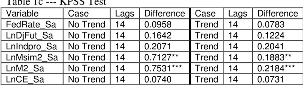
3.1. Unit Root Test... 25
3.1.1. Dickey and Fuller ... 27
3.1.2. Kwiatkowski, Phillips, Schmidt and Shin... 28
3.1.3. Variance Decomposition... 30
3.2. Vector Autoregression... 32
3.3. Cointegration Tests... 33
3.4. Impulse Response Analysis and Variance Decomposition... 35
3.5. Money Demand and Time Series Models... 39
4. EMPIRICAL RESULTS ... 45
5. CONCLUSION ... 57
REFERENCES ... 59
1.
INTRODUCTION
“So you think that money is the root of evil?” said Francisco d’Anconia.
“Have you ever asked that what is the root of money? Money is a tool of
exchange, which can’t exist unless these are goods produced and men able
to produce them. Money is the material shape of the principle that men who
wish to deal with one another must deal by trade and give value for money.
Money is not the tool of mockers, who claim your product by tears, or the
looters, who take it from you by force. Money is made possible only by the
men who produce. Is this what you consider evil?”1…
The modern theory on money demand incorporates the evolution of
financial markets behavior, and then of households’ allocation and
preferences in different fashions; innovation in money demand can be
considered as an increasing number of liquid assets between which to
choose, considering money as a store of value and as a mean of payment;
innovation modifies the utility of money holdings, through wealth and
substitution effects. Liquidity has to be weighted with risk aversion and
profitability to incorporate portfolio innovation properly (Oldani 2005).
The traditional approach to the transmission mechanism through which
money affects aggregate demand has focused on the key role of
interestrates. Monetary shocks upset money supply-money demand
equilibrium causing changes in interest rates. However, an important gap in
1The meaning of Money, Speech of Francisco d’Anconia , Atlas Shrugged, Any Rand,
this analysis is that while it is generally acknowledged that movements in
short-term interest rates like the Treasury Bill rate clear the money market,
aggregate demand depends primarily on long-term interest rates
(McCafferty). His paper represents an effort to link the traditional
macroeconomic literature on the transmission mechanism of monetary
shocks with the literature on the term structure of interest rates.
Cox, Ingersoll and Ross (1981) re-examines many of these traditional
hypotheses while employing recent advances in the theory of valuation and
contingent claims. They show how the Expectations Hypothesis and the
Preferred Habitat Theory must be reformulated if they are to obtain in a
continuous-time, rational-expectations equilibrium. They also modify the
linear adaptive interest rate forecasting models, which are common to the
macro-economic literature. The difference of this thesis is to represent an
effort to link the traditional macroeconomic literature on the transmission
mechanism of monetary aggregates with credit derivatives.
The main purpose of the thesis is to test the empirical validity of enriching
money demand function with credit derivatives using the new monetary
aggregates. Aftermath of Global Financial Crisis 2008 sparked off by
subprime mortgage crisis, the effects of derivatives on financial markets and
The name “new monetary aggregates” is attached to the Divisia monetary
aggregates and the CE indices. The aim is to introduce the theoretical
framework that the micro foundations approach to construct the new
monetary aggregates and introduce financial innovations. This is useful for
two reasons. First, the origins of the theoretical background are reviewed
and second, the theoretical framework for the empirical part of the thesis is
built. Then, a brief survey of monetary aggregation theory is given in
section 2.1. In section 3 the methodology is reviewed while in section 4
empirical results are analyzed for the in order to indicate the importance of
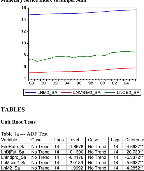
transmission mechanism on the development of credit derivatives. Empirical
results showed that Currency Equivalent Index and Monetary Service Index
are performing better than Simple Sum Monetary Aggregate.
The intensification of the global financial crisis, following the bankruptcy of
Lehman Brothers in September 2008, has made the current economic and
financial environment a very difficult time for the world economy, the
global financial system and for central banks. The fall out of the current
global financial crisis could be an epoch changing one for central banks and
financial regulatory systems. It is, therefore, very important that we identify
the causes of the current crisis accurately so that we can then find, first,
appropriate immediate crisis resolution measures and mechanisms (Mohan
The widespread innovations in the financial markets have brought important
changes in the way monetary policy is conducted, communicated and
transmitted to the economy. The transmission mechanism is changing.
While the effect of monetary policy on the availability and cost of bank
credit is decreasing, monetary policy actions have prompter effects on a
2.
LITERATURE SURVEY
This chapter is a brief survey of the monetary aggregation literature. The
main purpose is to introduce the theoretical framework that the micro
foundations approach uses to construct the new monetary aggregates.
Early attempts of weighted monetary aggregation studies are based on Hutt
(1963), Chetty (1969) and Friedman and Schwartz (1963) after it was
figured out that simple summation procedure have not been adequate
enough to capture the time dynamics of the asset demand theory. Then, the
concepts of the consumer’s choice problem, weak separability and
aggregator functions that explain the micro foundations of the new
monetary aggregates are discussed.
The fundamental theoretical argument of simple sum monetary aggregates is
that the owners of all monetary assets accept every asset as perfect
substitutes. With such simple summation including the milestone studies of
Diewert (1976) and Barnett (1978) divisia monetary aggregates and
Currency Equivalent Indices became popular under the “Micro foundations
approach” title. A weight of unity is attached to each monetary asset in
simple summation. However these assets have different opportunity costs.
As Barnett (1984) mentioned “one can add apples and apples, but not apples
Inadequate performance of money demand functions using simple sum
aggregates was questioned first by Goldfeld (1976). Once monetary assets
began yielding interest, these assets became imperfect substitutes for each
other. The missing money puzzle of Goldfeld (1976) was solved by Barnett
(1978, 1980) with the derivation of the user cost formula of monetary
services demanded. As a result, Barnett set the stage for introducing index
number theory in to the monetary economics.
Briefly, the Divisia index is a weighted sum of its components’ growth rates
where the weight for each component is the expenditure on that component
as a proportion of the total expenditure on the aggregate as a whole.
In many nations, monetary aggregates forms are expressed as M1, M2, M3
and L. Before Barnett (1978, 1980) many studies discussed the aggregation
of heterogeneous agents and also various goods a single agent purchases.
However, these approaches did not include microeconomic aggregation
theory and index number methods.
It is well known that the definition of the monetary aggregation affects the
structure of money demand and the transmission mechanism of the
economies. Hence, if the utility of monetary services is clearly
its’ important role for the causality relationships in the transmission
mechanism.
Therefore, this thesis will try to examine the importance of differences of
using Divisia index and simple sum method as monetary aggregator for
monetary policy and the transmission mechanism. In this sense, the main
goal is to analyze transmission mechanism models through time series
techniques. This will help to determine the nature of monetary policy
needed to combat financial crisis based on money supply and demand
dissonance during the subprime mortgage crisis period.
The rapid transmission of the U.S. subprime mortgage crisis to other
financial markets in the United States and other countries during the second
half of 2007 has raised some important questions. Frank et al. (2008)
suggest that during the recent crisis period the interaction between market
and funding liquidity sharply increased in U.S. markets
In contrast, these transmission mechanisms were largely absent before the
onset of financial turbulences in July 2007. The introduction of the
structural break in the long-run mean of the conditional correlations
between the liquidity and other financial market variables is statistically
2.1.
Consumer’s Choice Problem under Budget Constraints
of Monetary Assets
There have been consequences among economists. Economists agree on the
important roles of monetary assets in macroeconomics. Aggregation
methods should maintain the information contained in the elasticities of
substitution of monetary assets as well as abandoning strong a priori
assumptions about these elasticities of substitution. However, the widely
used simple sum monetary aggregates disregard the importance of
appropriate monetary aggregation methods as the ongoing discussion
demonstrates. An emerging literature employs statistical index numbers to
construct monetary aggregates that are consistent with microeconomic
theory.
Economists have agreed for a long time ago that equilibrium between the
demand for and supply of money is the most important long-run determinant
of an economy’s price level. Hence, it’s not such an easy case to measure
the aggregate quantity of money in the economy.
As simple summation method for monetary aggregates experienced flaws,
The Federal Reserve of St. Louis’ monetary services index project started to
provide researchers and policy makers with an extended and more efficient
database of new measures of monetary aggregates-the monetary services
Consumers hold monetary assets in order to obtain utility from various types
of monetary services. Some of these assets are more serviceable for
exchange as they reduce shopping time, permit sudden purchase of
bargain-priced goods and provide prevention against unanticipated expenses. The
demand of consumers for monetary assets on such cases can be considered
as a model of choices made by a representative consumer to maximize
utility function that is subject to a budget constraint. This budget includes
both stocks of real monetary assets and quantities of non-monetary goods
and services in which monetary assets are treated as durable goods that
provide a flow of monetary services.
In this context, Samuelson (1947) noted that;
… It is a fair question as to the relationship between the demand for money and the ordinal preference fields met in utility theory. In this connection, I have reference to none of the tenuous concept of money, as a numeraire commodity, or as a composite commodity, but to money proper, the distinguishing features of which are its indirect usefulness not for its own sake but for what it can buy, its conventional acceptability, its not being “used up” by use, etc.
Under these circumstances, for such a durable good its rental equivalent
the present value of the interest foregone by holding the monetary asset
discounted to account for the payment of interest at the end of the period.
2.1.1.
Optimization Problem of the Consumer
Every time the consumer makes a decision about monetary assets, he/she
faces an optimization problem under the budget constraints. In economics, a
central feature of consumer theory is about the choice that a consumer
makes. Just like in the theory of firm in which a firm decides how to
maximize costs, the consumer decision problem may be formalized by
assuming that the consumer maximizes the utility function,
(
m mn q qm)
U 1,..., , 1,... subject to the budget constraint:
∑
∑
= = = + m j j j i n i im p q Y 1 1π
where m=
(
m1,...mn)
is a vector of the stocks of real monetary assets(
π
π
n)
π
= 1,..., is a vector of user costs of monetary assets, q=(
q1,...,qm)
is a vector of quantities of non-monetary goods and services, p=(
p1,...,pm)
is a vector of prices of non-monetary goods and services, and Y is the
consumer’s total current period expenditure on monetary assets and
non-monetary goods and services.
All these decision problems have a feature in common. There is a set of
alternatives Ω from which the consumer has to choose. In our case, different
Briefly, a consumer in the theory of consumer behavior has a choice-set as
does the firm in the theory of firm. In this context, the consumer must have
some ranking over the different alternatives in the choice set. This ranking is
expressed by a real-value function such as f :Ω→ℜ where higher value of an alternative implies that it has a higher rank than an alternative with a
lower value.
In our model, these alternatives refer to monetary assets’ yield provided to
the consumer. In its abstract form an optimization problem consist of a set Ω
and a function2 f :Ω→ℜ. The purpose is to select an alternative from the set Ω that maximizes or minimizes the value of the objective function f.
That is the consumer either solves
i. Maximizes f
( )
w subject to w∈Ω orii. Minimizes f
( )
w subject tow∈Ω.As a result, the solution to the consumer’s optimization problem yields
demand function for real monetary assets and for quantities of
non-monetary goods and services:
(
p Y)
f mi* = i π, , for i=1,...,n and(
pY)
g q*j = jπ
, , for j=1,...,m2.1.2.
Barnett’s
Approach
over
Consumer’s
Optimization Problem
The simple sum monetary aggregates announced by the Federal Reserve are
calculated by summing dollar values of the stocks of the monetary assets
related to each aggregate which is not generally consistent with the
economic theory of the consumer’s optimization problem.
In the presence of such inadequate monetary aggregates, Barnett (1980)
developed a method which is quite consistent with the economic theory.
Barnett accepted the quantities of monetary assets included to the decision
maker’s portfolio as weakly separable from the quantities of other goods
and services.
In this context, the utility function U
(
m1,...,mn,q1,...,qm)
evaluated as(
)
[
u m mn q qm]
U 1,..., , 1,... where the function u
(
m1,...,mn)
represented the amount of monetary services the consumer received from the holdingportfolio of monetary assets.
As a result, under the assumption of weak separability, the marginal rate of
substitution between monetary assets mi and mj can be represented in terms
of the derivatives of u
(
m1,...,mn)
as;(
)
(
)
j n i n m m m u m m m u ∂ ∂ ∂ ∂ ,..., ,..., 1 1Barnett’s approach allows us to discuss the representative consumer’s
choice problem as if it were solved in two stages. In the first stage, the
consumer selects (1) the desired total outlay on real monetary services (but
not the quantities of individual monetary assets), and (2) the quantities of all
non-monetary individual goods and services. In the second stage, the
consumer selects the quantities of the individual real monetary
assets,m1,...,mn, conditional on the total outlay on monetary services
selected in the first stage, that provide the largest possible quantity of
monetary services.
This two-stage budgeting model of consumer behavior implies that the
category subutility function, u (m1,...,mn), is an aggregator function that
measures the total amount of monetary services received from holding
monetary assets. If we let m*1... m*n denote the optimal quantities of
monetary assets chosen by the consumer, we can regard the aggregator
function as defining a monetary aggregate, M, via the relationship
M = u(m*1,...,m*n). A major difficulty remains, however: The specific form
of the aggregator function is usually unknown. Diewert (1976) and Barnett
(1980) have established that, in this model, the aggregator function at the
M = u (m*1... m*n), may be approximated by a statistical index number. The
monetary services indexes presented in this issue of the Review are
superlative statistical index numbers, as defined by Diewert (1976).
Moreover, Serletis and Molik (2002) investigate the roles of traditional
simple-sum aggregates and recently constructed Divisia and currency
equivalent monetary aggregates in Canadian monetary policy to address
disputes about the relative merits of different monetary aggregation
procedures. They find that the choice of monetary aggregation procedure is
crucial in evaluating the relationship between money and economic activity.
In particular, using recent advances in the theory of integrated regressors,
they find that Divisia M1 + + is the best leading indicator of real output.
Furthermore, Divisia M1 + + causes real output in vector autoregressions
that include interest rates, and innovations in Divisia M1 + + also explain a
very high percentage of the forecast error variance of output, while
innovations in interest rates explain a smaller percentage of that variance.
In their paper Fleissig and Serletis (2002), provide semi-non-parametric
estimates of elasticities of substitution between Canadian monetary assets,
based on a system of non-linear dynamic equations. The Morishima
elasticities of substitution are calculated because the commonly used
Allen-Uzawa measures are incorrect when there are more than two variables.
Results show that monetary assets are substitutes in use for each other at all
2.2.
Money Demand Theories Survey
Money demand is an economic theme, which has fascinated economists
over the centuries and no unique result has been ever reached. As in the
models Baumol (1952), Tobin (1956), Stockham (1981) and Jovanovic
(1982), but in contrast to those of Grandmont and Younes (1973), and
Helpman (1981), households are allowed to hold interest bearing capital in
addition to barren money.
Moreover, money demand and money allocation in portfolio depend on the
definition of money and wealth and on the possible combinations,
depending on technology available and risk attitude. In particular there exist
a large number of potential alternatives to money, the prices of which might
reasonably be expected to influence the decision to hold money. Even so,
linear single-equation estimates of money demand with only a few variables
continue to be produced, in spite of serious doubts in the literature about
their predictive performance.
Stephen Goldfeld (1976) brought wide attention to the poor predictive
performance of the standard function. Another problem with this literature is
that the studies of the demand for money are based on official monetary
aggregates constructed by the simple-sum aggregation method.
Using very simple notation, we can synthesize the evolution of money
money
(
MV =PQ)
, moving to the Fisherian interpretation as( )
(
MV r =PQ)
and then consider the Keynesian liquidity preference(
)
(
Md = r,Y)
where money holdings are not only function of income (or consumption), but also depend on the alternative investment opportunities(following the speculative motive to hold money) together with
precautionary and transactions motives.
In this context, Tobin (1956) introduced the concept of average money
holdings
(
2)
12r bT
M = where b is the brokerage charge to convert bonds into money, r is the interest rate and T is the number of transactions.3
Money demand and its relationship with growth and inflation are central
themes in modern monetary such as Barro and Santomero (1972) and
Coenen and Vega (1999) who observe that a stable representation of the
money demand should include alternative assets’ return to explain portfolio
shifts and wealth allocations in the short run.
The simple Keynesian money demand function Md =
(
r,Y)
is enlarged with innovation( )
* r written implicitly as(
, , *)
r Y r Md = . Derivatives increase markets’ liquidity and substitutability as well as increasing thespeed of the transmission mechanism of monetary impulses. Although it is
possible to shift individual risk at the macro level it cannot be cancelled.
According to the credit view, the notion of imperfect substitutability
between credit and bonds and the introduction of derivatives that are highly
substitutable with bonds and credit, can dramatically alter the monetary
policy actions and effects in a market economy.
Since different functional forms have different implications for the presence
of the liquidity trap and effectiveness of the traditional monetary policy, the
choice of functional form is an important issue. Bae and De Jong (2007),
investigate two different functional forms for the US long-run money
demand function by linear and nonlinear cointegration methods. They aim
to combine the logarithmic specification, which models the liquidity trap
better than a linear model, with the assumption that the interest rate itself is
an integrated process. The proposed technique is robust to serial correlation
in the errors. For the US, their new technique results in larger coefficient
estimates than previous research suggested, and produce superior
out-of-sample prediction.
Finally Barnett et all. (2008), provide an investigation of the relationship
between macroeconomic variables and each of the Divisia first and second
moments, based on Granger causality. They find abundant evidence that the
Divisia monetary aggregates (or any Diewert superlative index) should be
used by central banks instead of simple sum monetary aggregates. This
by monetary policy makers, because they contain information relevant to
other macroeconomic variables.
2.2.1.
Thales of Miletus, First Derivative: Lagged
Application of an Original Idea
A derivative is a contract whose value depends on the price of underlying
assets, but which does not require any investment of principal in those
assets. (BIS 1995) Derivatives can be divided into 5 types of contracts:
Swap, Forward, Future, Option and Repo. These are financial instruments
widely used by all economic agents to invest, speculate and hedge in
financial market (Hull, 2002)
Unlike common belief, derivative instruments are not recent inventions. The
first account of an option trade contract is reported by Aristotle in his
Politics. In book1, Chapter 11 of Politics, Aristotle tells the story of Thales
(624-547 BC) who is said to have purchased the right to rent the olive
presses at a future point in time for a determined price. The main idea of
olive presses option was induced by the challenge of critics who had pointed
out to Thales’ poor material well being and mentioned that if the
philosopher had anything of value to offer others than he should be able to
get the respect he deserves. As Thales made a fortune of olive presses
contracts which turned the philosopher’s intellect to the creation of wealth.
Thales proved his cleverness but one point that needs to be mentioned is
Thales being a monopoly as there were no other bidders for the olive
olive presses at a very low price since there were no other bidders. Also
Aristotle illustrates the story of Thales as an operation of the monopoly
devise. Moreover, in their paper “What is the Fair Rent Thales Should Have
Paid” Markopoulos and Markelious (2005) try to calculate the ratio of the
option value to the market rental price of presses referring to Thales’ option
trade.
Likewise, in the 1600s in Amsterdam, both call and put options were written
on tulip bulbs during the legendary tulip-bulb craze. In 12th century, sellers
arranged contracts named “letters de faire” at fair grounds. These contracts
indicated the seller would deliver the goods he had sold on the determined
maturity. Commodities such as wheat and copper have been used as
underlying assets for option contracts in Chicago Commodity Exchange
since 1865. In 1900s, Bachelier began the mathematical modeling of stock
price movements and formulates the principle that “the expectation of the
speculator is zero” in his thesis Théorie de la Spéculation.
In this context, the origins of much of the mathematics in modern finance
can be traced to Louis Bachelier’s 1900 thesis on the theory of speculation,
framed as an option-pricing problem. This work marks the twin births of
both the continuous-time mathematics of stochastic processes and the
continuous-time economics of derivative-security pricing.
Furthermore, the mean-variance formulation originally developed by Sharpe
(1964) and Treynor (1961), and extended and clarified by Lintner (1965a;
(1965), Sharpe (1966) , and Jensen (1968; 1969) have developed portfolio
evaluation models which are either based on this asset pricing model or bear
a close relation to it. In the development of the asset pricing model it is
assumed that (1) all investors are single period risk-averse utility of terminal
wealth maximizers and can choose among portfolios solely on the basis of
mean and variance, (2) there are no taxes or transactions costs, (3) all
investors have homogeneous views regarding the parameters of the joint
probability distribution of all security returns, and (4) all investors can
borrow and lend at a given riskless rate of interest. The main result of the
model is a statement of the relation between the expected risk premiums on
individual assets and their "systematic risk.
Finally in 1997 Scholes and Merton won the Noble Prize in collaboration
with the late Fischer Black who developed a pioneering formula for the
valuation of stock options. It’s obvious that Thales pulled the trigger against
the notion “uncertainty” and inspired all other great minds for centuries in
order to be able to find a way to beat risk.
According to the conventional wisdom, credit derivative contracts are a
form of insurance. Henderson 2009 explores whether credit derivatives
should be regulated as insurance and offers an alternative form of regulation
for these financial instruments. The largely unregulated credit derivates
market has been cited as a cause of the recent collapse of the housing
market and resulting credit crunch. We regulate insurance companies with
insurance; (2) the unique governance problems inherent in a model in which
the firm's creditors are policyholders; and (3) a view that state-based
consumer protection is important to ensure a functioning market. This essay
shows that none of these policy justifications obtain in credit derivative
markets. The essay briefly discusses how a centralized clearinghouse or
exchange can help improve the credit derivatives markets, as well as
potential pitfalls with this solution.
2.2.2.
Derivatives in the Money Demand Function
The introduction of derivatives in emerging capital markets increases
international substitutability, attracting foreign investors (e.g. Tesobono
swap in Mexico). The dynamics of short-run broad money demand adjusts
to financial innovation, while the theory tells us that in the long-run money
should be a stable function of income and interest rate.
Money demand should be modeled through the use of weighted monetary
indexes such as Divisia Index, introduced in the literature. Divisia Index
addresses directly the problem of un-perfect substitutability contrary to
traditional money aggregates, which are simple sums of assets. The money
demand function in the implicit form can be written as (m/p) = f (r, y,
future), where (m/p) is real cash balance (money demand), and is a function
of interest rate (r), income (y), and the financial innovation (future)
representative of market and portfolios in terms of liquidity, and open
Nonexistent risk-free rate causes a risky economy in which derivatives are
by definition independent of their underlying assets and benefits from
specific pricing rules. The property of futures’ prices being correlated with
the underlying is efficiency characteristic and is called price discovery
effect4.
Discovery price effect should not be confused with the independency.
Generally speaking the introduction of exchange traded derivative products: i. Increases information about the underlying,
ii. Does not seem to increase volatility and risks of and on the
underlying market,
iii. Price discovery effect improves
iv. Bid-ask spread and the noise component of prices both decrease.
Although Reinhar et all. (1995), find that financial innovation plays an
important role in determining money demand and its fluctuations, and that
the importance of this role increases with the rate of inflation; Donmez and
Yilmaz (1999) state that “a mature derivatives market on an organized
exchange leads to a better risk management and better allocation of
resources in the economy”.
Central banks in certain circumstance use derivatives as a substitute of the
channels of monetary policy; Tinsley (1998) and others explain which
4
are the advantages for central banks in using derivatives to manage the
3.
ECONOMETRIC METHODOLOGY
Main purpose of this section is to review the econometric methodology used
in the empirical analysis followed by the empirical assessment of the
monetary aggregates for the developed countries.
The preferred empirical investigation procedure refers to time series, since
across countries (i.e. cross section) the definition of main variables is not
homogenous, leading to the complete lack of data and the impossibility of
any reliable analysis.
Panel data estimates are undeveloped in this field, since money demand
basically refers to non-stationary variables, and techniques and theory are
not yet able to deal with them. Time series analysis can be started, after the
check for the presence of unit roots. Macroeconomic variables are often
non-stationary, and the demand function should be expressed using the same
root order; i.e. if all variables are I(1) a function could be expressed in terms
of the levels; if one variable is I(2), we should take its first difference, which
is I(1), to estimate its parameter with other I(1) variables. Simple money
demand estimates on levels with the OLS provide unstable results and
Money demand estimates, being over long or short periods, have improved
fast after the Engle and Granger procedure evolved. Friedman and Schwartz
(1963) were the first to observe the existence of a strong correlation
between money supply and the business cycle, Tobin added that this causal
relationship could be reversed, and the Granger Causality test, introduced in
the field by Sims (1972), finally cleared the way. Barro, with many
co-authors, improved the analysis over the ‘70s, by discerning the influence of
real variables, shocks and un-anticipated components.
Modern money demand estimates can be split into short term analysis,
which use the error correction approach (ECM), i.e. the Maximum
Likelihood-ARCH estimator, and long term analysis, which use the Vector
Auto Regression (VAR) or the Vector Error Correction Mechanism
(VECM).
3.1.
Unit Root Test
The common procedure in economics is to test for the presence of a unit
root to detect non-stationary behavior in a time series. This thesis uses the
conventional Augmented Dickey-Fuller (ADF) for unit root tests.
In the terminology of time series analysis, if a time series is stationary, it is
said to be integrated of order zero, or I(0) for short. If a time series needs
one difference operation to achieve stationarity, it is an I(1) series; and a
stationarity. An I(0) time series has no roots on or inside the unit circle but
an I(1) or higher order integrated time series contains roots on or inside the
unit circle. So, examining stationarity is equivalent to testing for the
existence of unit roots in the time series.
A pure random walk, with or without a drift, is the simplest non-stationary
time series: ) , 0 ( ~ , 2 1 ε ε σε µ y N yt = + t− + t t (1)
where µ is a constant or drift, which can be zero, in the random walk. It is
non-stationary as Var yt =t →∞ ast →∞ 2
)
( σε . It does not have a definite
mean either. The difference of a pure random walk is the Gaussian white
noise, or the white noise for short:
) , 0 ( ~ , 2 ε σ ε ε µ N yt = + t t ∆ (2)
The variance of ∆yt is σε2 and the mean is µ.The presence of a unit root can
be illustrated as follows, using a first-order autoregressive process:
) , 0 ( ~ , 2 1 ε ε σε ρ µ y N yt = + t− + t t (3)
Equation (3) can be extended recursively, yielding:
(
)
(
)
t n n n t n n t t t t t t L L y y y yε
ρ
ρ
ρ
µ
ρ
ρ
ε
ρε
ρ
ρµ
µ
ε
ρ
µ
1 1 1 1 2 1 ... . 1 ... 1 . . . 2 − − − − − − − + + + + + + + + + + + + = + + = (4)where L is the lag operator. The variance of yt can be easily worked out:
( )
2 1 1 (σ
ερ
ρ
− − = n t y Var (5)It is clear that there is no finite variance for yt if ρ ≥ 1. The variance is
) 1 /( 2 ρ σε − when ρ< 1.
Alternatively, equation (3) can be expressed as:
(
L)
(
(
)
L)
y t t t − + = − + = ρ ρ ε µ ρ ε µ / 1 1 (6)which has a root r = 1/ρ.Comparing equation (5) with (6), we can see that
when yt is non-stationary, it has a root on or inside the unit circle, that is, r ≥
1; while a stationary yt has a root outside the unit circle, that is, r< 1. It is
usually said that there exists a unit root under the circumstances where r ≥ 1.
Therefore, testing for stationarity is equivalent to examining whether there
is a unit root in the time series. Having gained the above idea, commonly
used unit root test procedures are introduced and discussed in the following.
3.1.1.
Dickey and Fuller
The basic Dickey–Fuller (DF) test (Dickey and Fuller 1979, 1981) examines
whether ρ<1 in equation (3), which, after subtracting yt−1 from both sides,
can be written as:
(
)
t t t tt y y
y =µ + ρ− +ε =µ +θ +ε
The null hypothesis is that there is a unit root in yt, or H0 : θ = 0, against the
alternative H1 : θ< 0, or there is no unit root in yt . The DF test procedure
emerged since under the null hypothesis the conventional t -distribution
does not apply. So whether θ< 0 or not cannot be confirmed by the
conventional t -statistic for the θ estimate. Indeed, what the DF procedure
gives us is a set of critical values developed to deal with the non-standard
distribution issue, which are derived through simulation. Then, the
interpretation of the test result is no more than that of a simple conventional
regression. Equations (3) and (7) are the simplest case where the residual is
white noise. In general, there is serial correlation in the residual and ∆yt can
be represented as an autoregressive process:
t i i t t t y i y y µ θ φ ε ρ + ∆ + + = ∆
∑
= − − 1 1 (8)Corresponding to equation (8), DF’s procedure becomes the Augmented
Dickey–Fuller (ADF) test. We can also include a deterministic trend in
equation (8).Altogether; there are four test specifications with regard to the
combinations of an intercept and a deterministic trend.
3.1.2.
Kwiatkowski, Phillips, Schmidt and Shin
Recently, a procedure proposed by Kwiatkowski et al. (1992), known as the
KPSS test named after these authors, has become a popular alternative to the
ADF test. As the title of their paper, ‘Testing the null hypothesis of
stationarity against the alternative of a unit root’, suggests, the test tends to
test on the other hand, the null hypothesis is the existence of a unit root, and
stationarity is more likely to be rejected. Here in that the series yt is
assumed to be (trend-) stationary under the null. The KPSS statistic is based
on the the residuals from the OLS regression of yt on the exogenous
variables xt:
t t
t x u
y = 'δ + (9)
The LM statistic is defined as:
( )
(
)
∑
= t f T t S LM 2 2 0 (10)where, ƒ0 is an estimator of the residual spectrum at frequency zero and
where S(t) is a cumulative residual function:
( )
∑
= = t r r u t S 1 ˆ (11)based on the residuals ˆ '
δ
ˆ( )
0t t t y x
u = − . We point out that the estimator of δ
used in this calculation differs from the estimator for δ used by GLS
detrending since it is based on a regression involving the original data and
not on the quasi-differenced data.
To specify the KPSS test, you must specify the a set of exogenous
regressors xt and method for estimating ƒ0.
Many empirical studies have employed the KPSS procedure to confirm
rate and the interest rate, which, arguably, must be stationary for economic
theories, policies and practice to make sense. Others, such as tests for
purchasing power parity (PPP), are less restricted by the theory.
Confirmation and rejection of PPP are both acceptable in empirical research
using a particular set of time series data, though different test results give
raise to rather different policy implications. It is understandable that,
relative to the ADF test, the KPSS test is less likely to reject PPP.
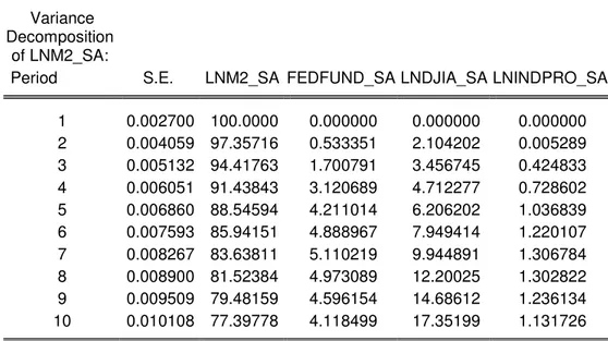
3.1.3.
Variance Decomposition
As returns may be volatile, we are interested in the sources of volatility. The
expression for innovation in the total rate of return:
{ }
(
)
(
)
∆ − − ∆ − = − ++ ∞ = + + ∞ = +∑
∑
τ τ τ τ τ τλ
λ
1 0 1 1 1 t t 1 t o t t t t E r E d E d r(
)
(
)
− − − − + ∞ = + ∞ = +∑
∑
τ τ τ τ τ τλ
λ
t t t t r E r E 1 1 1 1 1 (12)Equation (12) can be written in compact notations, with the left-hand side
term being νt, the first term on the right-hand side ηd, t, and the second term
on the right-hand side ηr, t:
t r t d t v =
η
, −η
, (13)where νt is the innovation or shock in total returns, ηd,t represents the
innovation due to changes in expectations about future income or dividends,
and ηr,t represents the innovation due to changes in expectations about future
innovations. Vector zt contains, first of all, the rate of total return or
discount rate. Other variables included are relevant to forecast the rate of
total return:
t t t Az
z = −1+
ε
(14)with the selecting vector e1 which picks out rt from zt , we obtain:
{ }
t tt t
t r E r e
v = − = 1'
ε
(15)Bringing equations (14) and (15) into the second term on the right-hand side
of equation (12) yields:
(
)
(
)
− − − = + ∞ = + ∞ = +∑
∑
τ τ τ τ τ τλ
λ
η
rt Et rt Et rt 1 1 1 , 1 1(
)
A t e(
)
A[
I(
)
A]
t eλ
τε
λ
λ
ε
τ τ 1 ' 1 ' 1 1 1 1 1 − ∞ = − − − = − =∑
(16)ηd,t can be easily derived according to the relationship in equation (13) as
follows:
(
)
[
(
)
]
{
}
t t r t t d vη
e Iλ
AIλ
Aε
η
' 1 , , 1 1 1 − − − − + = + = (17)The variance of innovation in the rate of total return is the sum of the
variance of ηr,t , innovation due to changes in expectations about future
discount rates or returns, ηd,t , innovation due to changes in expectations
about future income or dividends, and their covariance that is:
(
dt rt)
r d v Cov , , 2 , 2 , 2σ
σ
2η
,η
σ
= η + η − (18)3.2.
Vector Autoregression
The vector autoregression (VAR) is commonly used for forecasting systems
of interrelated time series. The VAR approach sidesteps the need for
structural modeling by treating every endogenous variable in the system as a
function of the lagged values of all of the endogenous variables in the
system.
The mathematical representation of a VAR is:
t t p t p t t t A y A y Bx y = −1 +...+ − + +
ε
where yt is a k vector of endogenous variables, xt is a d vector of exogenous
variables, A1,…., Ap and B are matrices of coefficients to be estimated, and is
ε
t a vector of innovations that may be contemporaneously correlated butare uncorrelated with their own lagged values and uncorrelated with all of
the right-hand side variables.
Since only lagged values of the endogenous variables appear on the
right-hand side of the equations, simultaneity is not an issue and OLS yields
consistent estimates. Moreover, even though the innovations may be
contemporaneously correlated, OLS is efficient and equivalent to GLS since
all equations have identical regressors.
As an example, suppose that industrial production (IP) and money supply
exogenous variable. Assuming that the VAR contains two lagged values of
the endogenous variables, it may be written as:
t t t t t t a IP a M b IP b M c IP = 11 −1+ 12 1−1 + 11 −2 + 12 1−2 + 1 +
ε
1 (19) t t t t t t a IP a M b IP b M c M1 = 21 −1+ 22 1−1 + 21 −2 + 22 1−2 + 2 +ε
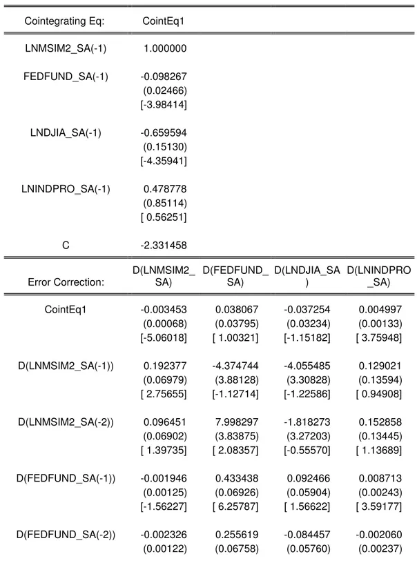
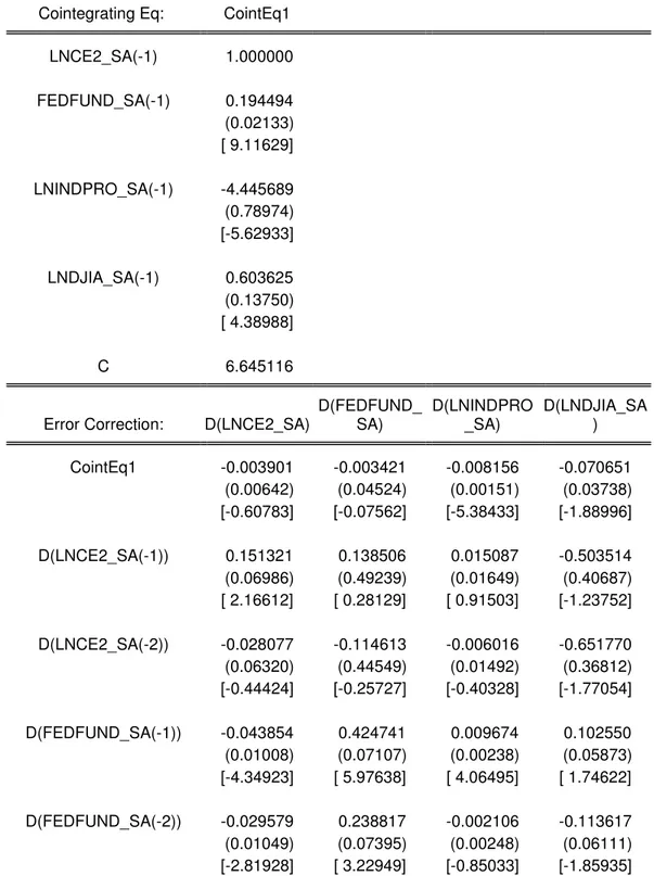
2 where, aij,bij and ciare the parameters to be estimated.3.3.
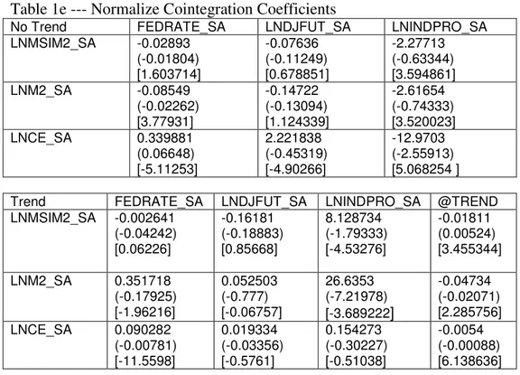
Cointegration Tests
The finding that many macro time series may contain a unit root has spurred
the development of the theory of non-stationary time series analysis. Engle
and Granger (1987) pointed out that a linear combination of two or more
non-stationary series may be stationary. If such a stationary linear
combination exists, the non-stationary time series are said to be
cointegrated. The stationary linear combination is called the cointegrating
equation and may be interpreted as a long-run equilibrium relationship
among the variables.
For a pair of variables to be cointegrated, a necessary (but not a sufficient)
condition is that they should be integrated of the same order. Assuming that
both xt and yt are I(d), the OLS regression of one upon another will provide
a set of residuals, ut. If ut is I(0) (stationary), then xt and yt are said to be
cointegrated (Engle and Granger, 1987). If ut is nonstationary, xt and yt will
tend to drift apart without bound. Therefore, cointegration would mean that
the cointegration of two variables is at least a necessary condition for them
to have a stable long-run (linear) relationship.
The Engle-Granger cointegration technique is a two-stage residual based
procedure. While quite useful, this technique suffers from a number of
problems. The purpose of the cointegration test is to determine whether a
group of non-stationary series is cointegrated or not. As explained below,
the presence of a cointegrating relation forms the basis of the VEC
specification. EViews implements VAR-based cointegration tests using the
methodology developed in Johansen (1991, 1995a).
Consider a VAR of order p:
t t p t p t t t A y A y Bx y = −1 +...+ − + +
ε
(20)Where yt is a k-vector of non-stationary I(1) variables, xt is a d-vector of
deterministic variables, and εt is a vector of innovations. We may rewrite
this VAR as,
t t i t p i i t t y y Bx y =Π +ΣΓ ∆ + +ε ∆ − − = − 1 1 1 (21) where o i p iΣA −I = Π =1 j p i j i 1A + =Σ − = Γ (22)
Granger's representation theorem asserts that if the coefficient matrix П has
reduced rankΓ<k, then there exist Γ×kmatrices α and β each with rank Γ such that Π=αβ'and β'yt is I(0).
Γ is the number of cointegrating relations (the cointegrating rank) and each column of β is the cointegrating vector. As explained below, the elements
of α are known as the adjustment parameters in the VEC model. Johansen's
method is to estimate the П matrix from an unrestricted VAR and to test
whether we can reject the restrictions implied by the reduced rank of П.
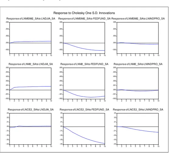
3.4.
Impulse Response Analysis and Variance Decomposition
Impulse response analysis is another way of inspecting and evaluating the
impact of shocks cross-section. While persistence measures focus on the
long-run properties of shocks, impulse response traces the evolutionary path
of the impact overtime. Impulse response analysis, together with variance
decomposition, forms innovation accounting for sources of information and
information transmission in a multivariate dynamic system.
Considering the following vector autoregression (VAR) process:
k k t k t t t A Ay A y K A y y = 0 1 −1 + 2 −2 + + − +µ (23)
where yt is an n × 1 vector of variables, A0 is an n × 1 vector of intercept, Aτ
(τ =1, …, k) are n×n matrices of coefficients, µt of white noise processes
with
( )
0,(
')
t tt E
E
µ
= Σµ =µ
µ
being non-singular for all t and,(
')
t tE µ µ for t≠s. Without losing generality, exogenous variables other than lagged yt are
omitted for simplicity. A stationary VAR process of equation (23) can be
τ τ τ
µ
µ
µ
µ
− ∞ = − −∑
Φ + = + Φ + Φ + + = t t t t t C K C y 0 2 2 1 1 (24) where C E( ) (
yt I A1 ... AK)
1A0 − − − − == and Φτ can be computed from Aτ
recursively K K A K A AΦ − + Φ − + + Φ − =
Φτ 1 τ 1 2 τ 2 τ , τ =1, 2, Λ with Φ0=I and Φτ forτ<0.
The MA coefficients in equation (24) can be used to examine the interaction
between variables. For example, aij,k, the ij th element of Φk, is interpreted
as the reaction, or impulse response, of the i th variable to a shock τ periods
ago in the j th variable, provided that the effect is isolated from the influence
of other shocks in the system. So a seemingly crucial problem in the study
of impulse response is to isolate the effect of a shock on a variable of
interest from the influence of all other shocks, which is achieved mainly
through orthogonalisation.
Orthogonalisation per se is straightforward and simple. The covariance
matrix
(
')
t t Eµ
µ
µ =
Σ ,), in general, has non-zero off-diagonal elements.
Orthogonalisation is a transformation, which results in a set of new residuals
or innovations vt satisfyingE
(
vt,vt')
=I. The procedure is to choose any non-singular matrix G of transformation for vt Gµ
t1 −
= so
thatG−1Σ G'−1 =I
µ . In the process of transformation or orthogonalisation,
Φτ is replaced by Φτ G and µt is replaced by vt =G−1
µ
t, and equation (24)( )
vv I E Gv C C yt = +∑
Φ t = +∑
Φ t t t = ∞ = − ∞ = − ' 0 0 τ τ τ, τ τµ
τ (25)Suppose that there is a unit shock to, for example, the j the variable at time 0
and there is no further shock afterwards, and there are no shocks to any
other variables. Then after k periods, ytwill evolve to the level:
(
G)
e( )
j C yt∑
k = Φ + = τ 0 τ (26)where e(j) is a selecting vector with its j the element being one and all other
elements being zero. The accumulated impact is the summation of the
coefficient matrices from time 0 to k. This is made possible because the
covariance matrix of the transformed residuals is a unit matrix I with
off-diagonal elements being zero. Impulse response is usually exhibited
graphically based on equation (26). A shock to each of the n variables in the
system results in n impulse response functions and graphs, so there are a
total of nxn graphs showing these impulse response functions.
To achieve orthogonalisation, the Choleski factorisation, which decomposes
the covariance matrix of residuals Σµ into GG’ so that G is lower triangular
with positive diagonal elements, is commonly used. However, this approach
is not invariant to the ordering of the variables in the system. In choosing
the ordering of the variables, one may consider their statistical
characteristics. By construction of G, the first variable in the ordering
explains all of its one-step forecast variance, so a variable which is least
to the first in the ordering. Then the variable with least influence on other
variables is chosen as the last variable in the ordering.
The other approach to orthogonalisation is based on the economic attributes
of data, such as the Blanchard and Quah structural decomposition. It is
assumed that there are two types of shocks, the supply shock and the
demand shock. While the supply shock has permanent effect, the demand
shock has only temporary or transitory effect. Restrictions are imposed
accordingly to realize orthogonalisation in the residuals. Since the residuals
have been orthogonalised, variance decomposition is straightforward. The
k-period ahead forecast errors in equation (24) or (25) are:
∑
− = − + − Φ 1 0 1 k k t Gv τ τ τ (27)The covariance matrix of the k-period ahead forecast errors are:
∑
−∑
= − = Φ Σ Φ = Φ Φ 1 0 1 0 ' ' ' k k GG τ τ τ µ τ τ τ (28)The right-hand side of equation (28) just reminds the reader that the
outcome of variance decomposition will be the same irrespective of G. The
choice or derivation of matrix G only matters when the impulse response
function is concerned to isolate the effect from the influence from other
sources. The variance of forecast errors attributed to a shock to the j the
variable can be picked out by a selecting vector e (j), with the j the element
(
)
( ) ( )
Φ Φ =∑
− = 1 0 ' ' ' , k G j e j Ge k j Var τ τ τ (29)Further, the effect on the ith variable due to a shock to the jth variable, or the
contribution to the ith variable’s forecast error by a shock to the jth variable,
can be picked out by a second selecting vector e(i) with the ith element
being one and all other elements being zero.
(
,)
( )
'( ) ( )
' ' () 1 0 ' i e G j e j Ge i e k ij Var k Φ Φ =∑
− = τ τ τ (30)In relative terms, the contribution is expressed as a percentage of the total
variance:
(
)
( )
∑
n= j Var ijk k ij Var 1 , (31)which sums up to 100 per cent.
3.5.
Money Demand and Time Series Models
Non-stationarity of time series data, an important characteristic of time
series, has been taken care of by the theory of cointegration. Whereas the
question as to whether the estimated model is valid for statistical inference,
forecasting and policy analysis or not is addressed by the theory of
exogeneity.5 It is strongly argued that the analysis of exogeneity of
parameters of interest is required to derive policy implications from the
cointegration analysis. The exogeneity of variables depends upon the
parameters of interest and the purpose of the model. If the model is to be
used only for statistical inference/analysis then we require the analysis of
weak erogeneity. If the purpose of modeling is forecasting the future
observations then we need to conduct the analysis of strong exogeneity.
Finally the concept of super-exogeneity is relevant if the objective of the
study is that the money demand model to be used for policy analysis.
Considering the importance of money demand in the macroeconomic
analysis and exogeneity in statistical analysis, forecasting and policy
simulation, this paper attempts to provide congruent money (M2) demand
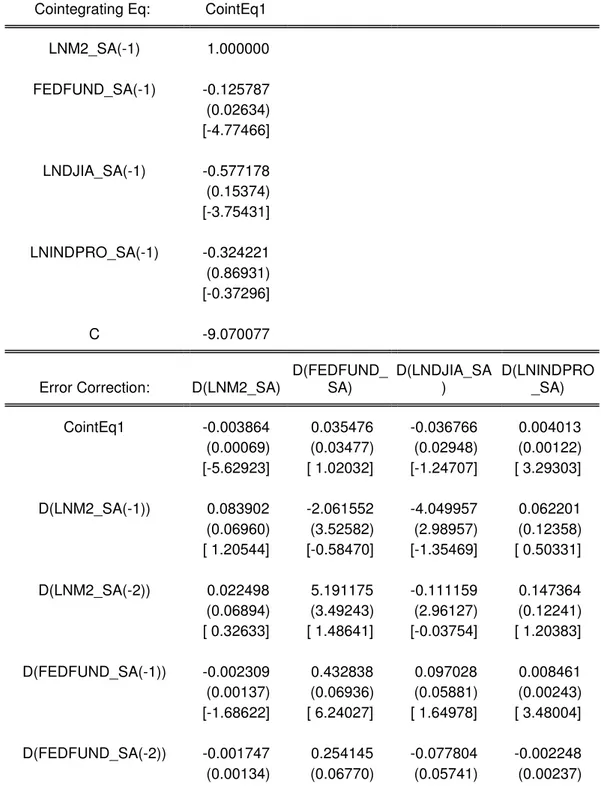
function by employing cointegration analysis, estimating dynamic error
correction model and testing the super-exogeneity of the parameters of
interest.
The error correction model has become a very popular specification for
dynamics equation in applied economics, including applications to such
mainstream problems as personal consumption, investment, and the demand
for money. The statistical framework is attractive, in that it encompasses
models in both levels and differences of variables and is compatible with
long-run equilibrium behavior. The success of the error correction paradigm
in applications has led to the development of theory justifying the form of
such an estimating for purposes of interference (i.e. the concept of
cointegration in economics time series-Granger and Engel (1988), and
related literature), as well as discussion of the theoretical behavior of such
With the introduction of derivatives, markets are more perfect thus
influencing monetary policy actions (Vrolijk, 1997). Financial innovation
influences the structure and behavior of the central banker, and the
process of development of financial markets goes together with the
process of changing of monetary theory and policy.
Financial innovation might influence the degree of substitution between
financial assets in the portfolio of economic agents. We treat this property in
a Tobin’s framework (Savona, 2003). Given more perfect financial market,
the substitutability between financial assets and liabilities increases, thus
making the traditional demand for money function unstable in its
parameters, which do not include innovation.
The introduction of derivatives on world markets decreases asymmetries,
transaction and investment costs, thus contributing to increase the
possibilities for portfolio diversification. The degree of substitution with
traditional and new investments increases, making money aggregates less
meaningful
In this context, the money demand function defined in the previous sections
should be implemented according to the country specific conditions based
on empirical investigation procedure that refers to the time series, since
across countries the definition of main variables is not homogenous. This