Assembly line balancing problem: Comparison of some heuristic procedures

и т т й і і № » ш і Ѣ з Ш і г і - і т ш *1 А « ні М Ч£/ « '-«виг ^ І І Ш й Т Т і , Ё “Τί^ ы ш ш ' м ^ ^ - i: i » i , - «гчгі^ W -■ *1 J W >í*ííf¿í J .'^- W J£ ''Í¿ -' w 'S 5 ^3 w iM .··'^ ’^ J^’lJ^'J^i^Jwl; J.w'-^i - w^ VaTv* i í ' i ^ V · . , ' â y m z à b - т - ^ ш ш Н .:vv..- - --■■ ■^;»<*■ı-Λ·^'>лı^^ 'i l > 11^(3*)2 ' < t ¿ ^ f - 3 C i^ ' ' ^ ‘^ • • > ip '« a  t./ s e ^ ' ^ ' ü ѵ Ч л » .' ..'. '•t ’s e ^ W ’ii» « Ü ».W VblÎ 'лі} ,ΰί. < f í , ^ - f - · . "И s-f v: i. .J ^ H ü

З о -

₂

-Э

ASSEMBLY LINE BALANCING PROBLEM: COMPARISON OF SOME HEURISTIC PROCEDURES

IN

A THESIS

SUBMITTED TO THE DEPARTMENT OF MANAGEMENT AND THE GRADUATE SCHOOL OF BUSINESS ADMINISTRATION

OF BILKENT UNIVERSITY

PARTIAL FULFILLMENT OF THE REQUIREMENTS FOR THE DEGREE OF MASTER OF BUSINESS ADMINISTRATION

By

HASAN ALI METE OCTOBER, 1989

HD 3 0 - 2 9

(У,Б65 I Я ^ 3

I certi-fy that I have read this thesis and in my opinion it is -Fully adequate, in scope and in quality, as a thesis -for the degree of Master of Business Administration.

Assist. Prof. Erdal Erel

I certify that I have read this thesis and in my opinion it is fully adequate, in scope and in quality, as a thesis for the degree of Master of Business

Administration-I certify that Administration-I have read this thesis and in my opinion it is fully adequate, in scope and in quality, as a thesis for the degree of Master of Business Administration.

Assist. Prof. Kur^at Aydogan

Approved for the Graduate School of Business Administration

Prof. Dr. Subidey Togan

ABSTRACT

ASSEMBLY LINE BALANCING PRÜBLEM: CONPARISÜNS OF SONE HEURISTIC PROCEDURES

HASAN ALI NETE

Master of Business Administration Supervisor: Assist.Prof. Erdal Erel

October 1989, 58 pages

Assembly line balancing problem can be defined as assigning tasks to an ordered sequence of stations, such that the precedence relations among the tasks are satisfied and some pel- hormarice measure (e.g. toLal idle tune; is opLimized- in this work, some heuristic methods are examined and compared for an 11-element assembly line balancing problem for fixed F-ratios and cycle times. The results of the experiments show that there is no significant difference between the four selected heuristic procedures.

Keywords: Assembly Line Balancing Problem, Heuristic Procedure, Work Element, Balance Delay Ratio

ÖZET

SERÎ ÜRETİM HATTI DENGELEME PRÜBLEMI: BAZI HEURISTIC ÇÖZÜMLERİN KARŞILAŞTIRILMASI

HAŞAN ALI METE Yüksek Lisans Tezi

Tez Yöneticisi: Y.Doç.Dr- Erdal Erel Ekim 1989, 58 say-Fa

Seri üretim hattı dengeleme problemi, is elemanlarının belli sıra halindeki istasyonlara atanması olarak tanımlanır. Bu. esnada is elemanları arasındaki öncelik ilişkileri yerine getirilir ve toplam is zamanı gibi bazı performans ölçüleri optimize edilir- Bu çalışmada, bazı heuristic metodlar incelenip, F~oranları ve is çevrim zamanları sabit tutularak, 11 is elemanından oluşan seri üretim hattı dengeleme problemi için kıyas 1ama 1arı yapılmıştır. Denemelerin sonucunda, seçilen 4 heuristic yöntem arasında belirli bir fark olmadığı gözlenmiştir.

Anahtar Kelimeler: Seri üretim Hattı Dengeleme Problemi, Heuristic Yöntem, İs Elemanı, Dengeleme Gecikme Oranı

ACKNOI

JLEDGENEN

I would like to express my gratitude to Assist. Prof. Erdal Erel for his patient supervision. I am also grateful to Assist. Prof. Dilek Yeldan, and Assist. Prof. Kur^at AydoQan for their suggestions which greatly aided in the completion of this thesis.

T A B L E OF CQi I i Ei i i'S Page ABSTRACT i i i ÖZET 1 V ACKNOWLEDGEMENT V TABLE OF CONTENTS V i LIST OF TABLES i X LIST OF FIGURES X LIST OF SYMBOLS X 1 CHAPTER 1. INTRODUCTION 1 1.1. BACKGROUND 1

1.2. THE ASSEMBLY LINE BALANCING PROBLEM i

1.3. PURPOSE OF 1 HE THESIS 2*

1.4. OUTLINE OF THE THESIS 2

CHAPTER 2. DETERMINISTIC (CLASSICAL) LINE BALANCING 3

2.1. ASSEMBLY LINE DEFINITIONS o-5»

2.1.1. Work Station 3

2.1.2. Minimum rational uviork e 1ement 3 2.1.3. Total Work Content, Total Work

Content T i me 3

2.1.4. Cvcle T ime 4

2.1.5. Station Time, Station Work Content

T i me 5 _Balance D e lay 2_^_1.^7^^_Precedence Diagram 5 6 V 1

2 . - _ . C L _ Z-.8qu qtie

Eü ® £ §. .d e 12 c e _ h a.t r_ i ,,z ^ 2^]i_._9 ._The Task F 1 e x i b i l.i ty _Ra^i_p_-_.F_Rati^o 8 2.2. THE CLASSIC DETERİİ IN IS T IC LINE BALANCING

PROBLEM 8

CHAPTER 3. REVIEW OF RELATED RESEARCH 11

3.1. HISTORICAL REVIEW 11

3.2. THE ALB RESEARCH CLASSIFICATION: 15

CHAPTER 4. EXPERIMENTAL DESIGN 18

4.1. VARIABLES OF THE PROBLEM 18

4_^_1_^X^_JİI!®_AşBembJ^y_Taşj<_Şi^e_(Prob 1 em

Ş İ 2el 18

4^1^2_;_The Prec e dence Rela t ionship

1

4^1^3 j^_T he_ÇYÇJ.e_ Jlme 21

4^1j_4j;_The Work Element Times 22

4.2. PERFORMANCE MEASURE OF THE SOLUTION

EFFICIENCY 23

4.3. THE SELECTED HEURISTIC PROCEDURES 23 CHAPTER 5. ANALYSIS OF THE SELECTED METHODS AND SAMPLE

SOLUTION FOR EACH OF THEM 24

5.1. HEURISTIC METHOD DEVELOPED BY M. KILBRIDGE

AND L. WESTER 24

5.2. HEURISTIC METHOD BY W.B HELGESON AND

D.P. BIRNIE 26

5.3. HEURISTIC METHOD OF IMMEDIATE FOLLOWERS 27 5.4. HEURISTIC METHOD OF NUMBER OF FOLLOWERS: 28

CHAPTER 6. EXPERIMENTAL RESULTS AND EVALUATION AMONG METHODS 29 CHAPTER 7. CONCLUSION 33 APPENDIX A 35 APPENDIX B 39 APPENDIX C 49 REFERENCES 56 V 1 1 1

LI ST GF TABLES

Table 1. Balance Delays for Fixed F-ratios and Cycle Times

Table 2. Computation Results of ANOVA Method

Page

30 31

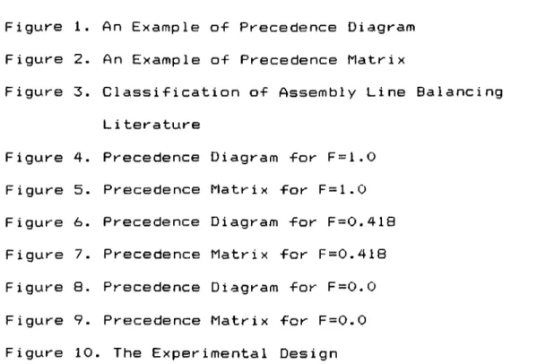
Page Figure 1. An Example of Precedence Diagram 6 Figure 2. An Example of Precedence Matrix 7 Figure 3. Classification of Assembly Line Balancing

Literature 16

Figure 4- Precedence Diagram for F=1.0 19 Figure 5- Precedence Matrix for F=1.0 19 Figure 6- Precedence Diagram for F=0.418 20 Figure 7- Precedence Matrix for F=0-418 20 Figure 8. Precedence Diagram for F=0-0 21 Figure 9. Precedence Matrix for F=0.0 21

Figure 10. The Experimental Design 22

LI S T OF S Y M B O L S

m: total number of work elements to complete a product tj^: work element time for the work element

tmax" íTiaximum work element time W: total work content time

C: cycle time

T*: a given time duration (period) Q: number of units to be assembled

station work content time oir station n d*: Balance delay ratio

dp: Idle time for the station n

d: Total idle time for per unit of product on the line C: average cycle time

N: Total number of work stations

H: Total number o f zeros in the half matrix of the precedence matr i x

u ^ z m o a n balance delay

CHAPTER 1 1. INTRODUCTION

1.1. BACKGROUND

In the early 1900's, Henry Ford began experimenting with a new concept in the division of labor. Using an idea originating from the overhead troiley of the Chigago meat patchers, Ford introduced the concept of an assembly line to the production of automobiles. As a result of his original work, the number of assembly lines rapidly increased and today they are used in most areas of i ndustry.

One of the problems Ford encountered was inefficient balance of assembly lines during the operation. The inefficiency of operations in assembly lines caused to search special solutions for these problems.

1.2. THE ASSEMBLY LINE BALANCING PROBLEM

In its basic form, an assembly line consists of a finite set of work elements or tasks, each having an operation processing time and a set of precedence relations.(8) The process of assigning tasks to an ordered

sequence of stations, such that the precedence relations are satisfied and the total idle time is minimized, is often called the "Assembly Line Balancing Problem".

1.3. PURPOSE OF THE THESIS

The "Assembly Line Balancing" is chosen as a subject for the thesis because use of assembly lines are increasing everyday in most of the industries. This thesis is based on the comparison of four heuristic procedures to solve the classical assembly line balancing problem. In addition, this heuristics will be analyzed to see which one gives the best results over the others.

1.4. OUTLINE OF THE THESIS

Chapter II states the classical assembly line balancing problem and related definitions, while Chapter III reviews the literature. Chapter IV considers the design and some performance measures of the problem. Analysis of selected heuristic methods and a solution for each are presented in Chapter V. Evaluation of the results and comparison of the procedures are given in Chapter VI. The conclusions of the research and recommendations for further study are presented in Chapter VII.

CHAPTER II

2. DETERMINISTIC (CLASSICAL) LINE BALANCING

2.1. ASSEMBLY LINE DEFINITIONS 2.1.1. Ulork Station

A work station is a location on the assembly line where an operator performs a given amount of assembly work.

In general, work stations are operated by a single operator.

2.1.2. Minimum rational work element:

A work element is a rational division of work. In practice, work elements are considered as indivisible since it is not possible to assign a work element to two or more

operators without increasihg costs and decreasing

productivity. Work element time is the time required for the accomplishment of a rational work element. A work element time is represented by t^^ where i is the work element, i=l,...,m.

2.1.3. Total Work Content, Total Work Content Time:

Total work content is the total of operations required to assemble a product. Total work content time is the time

cor respondí ng to the assembly of a product- The total lAjork content time is represented by W, where

m W = E t ¿ .

i = l

2_j_j[j^4j^_Cycie_Tj^me

In general, cycle time is the time allowed to each operator for the performance of certain jobs on the product- It includes both productive and non-productive as well as any idle time. Cycle time is defined in several ways: "Cycle time is the amount of time elapsing between successive units as they move down the line at standard pace."(16) "The amount of time a unit of product being assembled that is normally available to an operator performing his assigned task."(21)

Cycle time is represented by C. A lower bound on cycle time is the maximum work element time (t^^^). An upper bound on C is imposed by the demand rate (D) ; the reciprocal of demand rate constitutes an upper bound. That

2-1.5- Station Time, Station Work Content Tj^rne

Station time (service time) is the actual time correspondi ng to the performance of woK'k elements assigned to a work station. Station time for station n is represented by S^^- Station time is limited by maximum work element time (t^^^) and cycle time

C-tmax <n)< < C for all n

_BaJ^ance_DeJ^ay^

Balance delay is the amount of idle time on the assembly line caused by the imperfect division and assignment of work elements to the stations-(16) In a perfectly balanced line S^^ = C for all n and there is no balance delay- Since such cases are very rare, balance delay is almost always present in the assembly line balancing problems. Idle time is used as a measure of the degree of imbalance and is represented by d^ for station n.

The degree of imbalance is also measured by balance delay ratio which is defined as follows:

d* = 100 C - C = 100 NC - Etj NC (2.1.6.1)

w h e r e

C : cycle time

C : average cycle time, C =

N : number of work-stations

Et, N

(2.1.6.2)

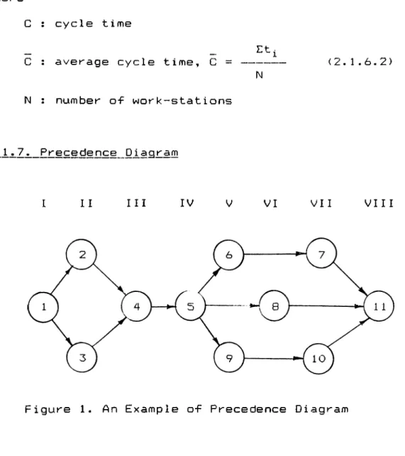
__Pr ecedence__Dj ^a32iarn

I II III IV V VI VII VIII

Figure 1. An Example of Precedence Diagram

A precedence diagram is a tool used in assembly line balancing. Its basic purpose is the représentâtion of the actual assembly line by completely describing work elements and their order of performance. The precedence diagram for an 11- task assembly line is given in Figure 1. The preparation of precedence diagrams and the rules are explained in detail in Appendix A.

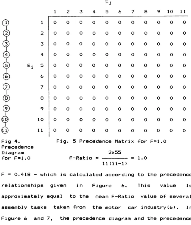
_P^^ecedence Matrix - Square Precedence Matrix

The precedence matrix is an mxm matrix which indicates the precedence re 1 a t i onsh i ps o-F the tasks. The llxii matrix given in Fig. 2., is -for the precedence diagram given in Fig. 1

-In this matrix, all the elements are listed on the top and left margins. In a cell correspond!ng to the row of element i and column of element j, +1 indicates that the element i will precede element j, -1 indicates that element i will follow element j, and 0 indicates that there is no relationship between elements i and j.

Element j Element i 1 2 3 4 5 6 7 8 9 10 11 1 0 1 1 1 1 1 1 1 1 1 1 2 -1 0 0 1 1 1 1 1 1 1 1 3 -1 0 0 1 I 1 1 1 1 1 1 4 -1 -1 -1 0 1 1 1 1 1 1 1 5 -1 -1 -1 -1 0 1 1 1 1 1 1 6 -1 -1 -1 -1 -1 0 1 0 0 0 1 7 -1 -1 -1 -1 -1 -1 0 0 0 0 1 8 -1 -1 -1 -1 -1 0 0 0 0 0 1 9 -1 -1 -1 -1 -1 0 0 0 0 1 1 10 -1 -1 -1 -1 -1 0 0 0 0 0 1 1 1 -1 -1 -1 -1 -1 -1 -1 -1 -1 -1 0

The F-ratio is a comparative indicator of the number of feasible sequences that could be generated from the m element-assembly t a s k . (6) The ratio characterizes the precedence structure of an assembly task.

_t

j^o_-_F_Ra

t^o

If H is the number of zeros in the half matrix of the precedence matrix, then the F-ratio is defined as

F-ratio = FI / Total number of cells in the partial matrix 2 H

m (m - 1)

(2.1.9.1)

F-ratio can range from 0 for assembly tasks ordered serially, to 1 for work elements having no precedence relationships.

2.2. THE CLASSIC DETERMIN IST IC ;LINE BALANCING PROBLEM

In the classical assembly line balancing problem, the following are given:

1. A set of tasks which comprises the production unit along with the associated task performance times tj^,

(i = 1,...,m ) .

2. A set of precedence relationships that define the order in which tasks can be performed.

3. A cycle time, C, which is determined from the desired output rate.

If the station time is less than the cycle time, then the worker is idle for some part of the cycle. Thus the difference between the station time and the cycle time is the “idle time" for a particular station. The idle time for station n is denoted by d^^ where d^^ = C ~ S^. Then the total idle time (d) per unit on a line with N stations would be

N N N

d = E d^ = E (C - S^) = NC - E

n=i^ n=l ^ n=l^ (2.2.1)

Since the sum o-F the work assigned to all work stations is the work content time, we have

N m

E = E t. = W

n=l^ i=l^ (2.2.1)

The objective is to minimize the total idle time subject to the precedence relationships and the cycle time requirement; i.e. the station time cannot exceed the cycle time. The objective can be formulated as;

min d = min (NC - mE t. ) i = l ^

min d = min (NC - W) = (C m i n N - W) such that S|^ < C for all n = 1,...,N and the precedence relations are not violated.

It can be concluded that for a fixed cycle time, minimizing idle time is equivalent to minimizing the number of work stations- A 1 ternative1y , for a fixed number of stations, minimizing idle time is equivalent to minimizing the cycle time. Both approaches are used in the literature but the most common approach, and the one to be taken in this research, is to assume that the cycle time, C, is prespecified to correspond to a desired production

rate-L·/ getting this objective, following constraints should be satisfied;

1. Each work element is assigned to a single work station 2. The precedence relations are not violated

3. The desired cycle time is not

CHAPTER III

3. REVIEW OF RELATED RESEARCH

3.1. HISTORICAL REVIEW

By the use o-F product layout and progressive assembly lines, large volume of goods are produced in relatively short time once the production and/or assembly lines are establi shed.

The line balancing problem has been initially defined by Benjamin Bryton(4) in his Master’s thesis completed in 1954. Bryton assumed the number of work stations to be constant and by interchange of work elements between stations he tried to minimize balance delays and obtain station times converging to a common value. The same principle is later used by Moodie and Young(20) who designed Bryton’s system for computer usage. Their program is a two-phase procedure for line balancing. In the first phase, an initial balance was achieved using the "largest candidate rule". This rule assigned tasks to stations by always selecting the task with the largest performance time which did not violate the precedence and cycle time restrictions. In the second phase, heuristic procedures were used to shift tasks between stations in order to reduce idle time. Moodie and Young then showed how to apply

their algorithm when task times were considered as random variables·

Sa 1 veson's (23 ) research on the subject is the -first published procedure on the line balancing problem. Although the method developed by Salveson is experimented easily -for a few work element ALB problem, it gets quite complicated as the number of work elements increases. Salveson has also developed a linear programming technique that has a matrix '’enormously large" and for practicaJ problems "сотри tat iona11 у unfeasible".

In 1956 James Jackson(13) developed a method based on the enumeration of all feasible assignments to work stations- Using the rules given by Jackson, a selection between the feasible station assignments is made taking into consideration the selected cycle time. Finally, the assignment for which the number of stations is minimum is selected. Although this method provides an optimal solution, it requires a computer.

E. H. Bowman(3) has developed two separate linear programming models to the balancing of assembly lines. Both of these models have large сотриtationa1 requirement, for problems of even modest size. For a simple problem with 8 work elements, the method requires the solution of 135 constraint equations with 112 variables. Bowman^s method has an academic rather than practical value.

üne of the first methods which is cornpu ta t i ona 1 1 у practical for manual balancing is the one developed by Helgeson and Birnie(lO). This method is called “Ranked Positional Weight Technique" where each work element is given a weight and assignment to work stations is made in the descending order of positional weights.

The process of reducing alternative grouping of tasks to stations with special rules and approaches which is more improved over traditional trial and error methods, are often called "Heuristic Procedures". Heuristic Procedures do not guarantee an optimum solution-(25) The first Heuristic Line Balancing procedures are those developed by Kilbridge and Wester (16), (17) and Tonge (26), (27).

The heuristic procedure developed by Kilbridge and Wester(16) is a very simple method requiring little knowledge of elementary arithmetic- This procedure does not require the use of computers and provides a manual solution to the Assembly Line Balancing problem.

Tonge"s(27) heuristic method attempts tries to solve the line balancing problem in three steps- In the first step, elements which are adjacent in the precedence diagram are grouped into compound tasks. In the second step, the newly formed compound tasks are assigned to work stations. Finally, in the third step elemental tasks are transferred

-From station to station until an even d i s t r i but i on of work is achieved·

The heuristic technique developed by Hoffman(ll) made use of a precedence matrix. His iterative procedure enumerated all feasible combinations of tasks that could be assigned to a station and then selected that combination of tasks which minimized the idle time at each successive station.

Kiein(18) described a procedure for finding an optimal assignment of tasks to work stations once the order of the tasks was specified· Since the method considers all feasible sequences, it can only be practically applied to smal1 problems.

Gutjahr and Nemhauser(9) developed an algorithm for the classical problem as a shortest route problem. The general procedure was to construct a network model where the arcs represented work stations and the nodes corresponded to possible first station assignments. The arc lengths corresponded to idle times and the optimization procedure found the shortest path in the network which corresponded to the minimum idle time.

A r c u s (2) developed a technique called COMSOAL (Computer Method of Sequencing Operations for Assembly Lines). The basic idea is the random generation of a large

number of feasible sequences based on hieuristic rules which favorably bias the selection of tasks by weighting them. As each sequence is generated, tasks can be assigned to work stations in accordance with the cycle time. Then a feasible sequence which gives the least number of work stations is selected.

Mansoor(5),(6) developed and improved the Helgeson and Birriie's Ranked Positional Weight Technique. His basic variation was to keep track of the total idle time as the RPW method was applied. If the total idle time exceeded some prespecified value, then backtracking took place.

Besides the single model assembly line“ balancing techniques, several authors have proposed techniques for mixed model lines.

3-2. THE ALB RESEARCH CLASSIFICATION:

ALB problem and the accompanying research can be classified into four categories as depicted in Figure 3.; Single Model Deterministic (SMD), Single Model Stochastic

(SMS), Multi/Mixed Model Deterministic (MMD), and Multi/Mixed Model Stochastic (MMS).

ALB LITERATURE Single Model Deterministic (SMD) Stochastic (SMS) Multi/Mixed Model Deterministic (MMD) Stochastic (MMS)

Figure 3. Classification of Assembly Line Balancing L i terature

In SMD version of ALB which is going to be analyzed in detail in further sections, task times are known deterministicaIly. This is the original and simplest form of the assembly line balancing, problem.

The SMS problem category introduces the concept of task time variability. This is more realistic for manual assembly lines, where workers’ operation times are seldom constant.

With the introduction of stochastic task times many other issues become relevant, such as station times exceeding the cycle time, pacing eFfects on workers’

operation times, station lengths, the size and location of inventory buffers, launch K-ates, arid allocation of line i mbalances.

The MMD problem formulation assumes a single line capable of producing multiple products with deterministic task times. Multi-model lines assemble two or more products seperately in batches. In contrast, in mixed-model lines single units of different models can be introduced in any order or mix to the assembly line for the purpose of preventing the overlap of the two definitions, it is convenient to consider both types within a single category. Multi/mixed model lines introduce various issues that are not present in the single model case- Model selection, model sequencing and launching I'ateisi, and model lot sizes become more critical issues here than in the single model case.

In MMS case, stochastic task times are allowed. All of the problems arising from SMS problem are valid here. However, these issues become more complex for the MMS problem because factors such as learning effects, worker skill level, job design and worker task time variability become more difficult to analyze because the line is frequently rebalanced for each model assembled.

CHAPTER IV

4. EXPERIMENTAL DESIGN

4.1. VARIABLES OF THE PROBLEM

Variables in Assembly Line Balancing problems occur either as -Functions o-F the assembly task, or as -Functions of the balancing requirements. Main factors of the assembly task were considered as being: the task size, the precedence relationships and their distribution, work element times and their distribution, and cycle time. In this experiment, F-ratios and cycle times were held constant against each heuristic.

4.1.1. Assembly Task Size (Problem Size)

The sample problem which was selected from E.J. Ignall’s(12) paper has 11 work elements, (see Figure 6)

4.1.2. ____Precedence Relationship (F-ratio)

Three levels of F-ratio were selected:

F = 1.0 - which should provide all feasible sequences for the assembly task.

T h e p r e c e d e n c e d i a g r a m a n d t h e p r e c e d e n c e m a t r i x -for F = l - 0 a r e s h o w n i n F i g u r e 4 a n d 5, r e s p e c t i v e 1 y , Ej 7 8 10 11 1 2 3 4 5 6 7 8 9 10 11 0 O O O O 0 0 0 0 0

o

o

o

o

o

o

o

o

o

o

o

o

o

o

o

o

o

o

o

o

o

o

o

o

o

o

o

o

o

o

o

o

o

o

o

o

o

o

Fig. 5 Precedence Matrix for F=1.0 2x55

F-Ratio = = 1 . 0

1 1 ( 1 1 - 1 )

F = 0.418 - which is calculated according to the precedence

relationships given in Figure 6. This value is

approximately equal to the mean F-Ratio value of several assembly tasks taken from the motor car industry(6). In Figure 6 and 7, the precedence diagram and the precedence matrix for F = 0.418 are presented,respect!vely.

1 2 3 , 4 5 6 7 8 9 10 11 1 0 1 1 1 1 1 1 1 1 1 1 2 -1 0 0 0 0 1 0 1 0 1 1 3 -1 0 0 0 0 0 1 0 1 0 1 4 -1 0 0 0 0 0 1 0 1 0 1 5 -1 0 0 0 0 0 1 0 1 0 1 6 -1 -1 0 0 0 0 0 1 0 1 1 7 -1 0 -1 -1 -1 0 0 0 1 0 1 8 -1 -1 0 0 0 -1 0 0 0 1 1 9 -1 0 -1 -1 -1 0 -1 0 0 0 1 10 -1 -1 0 0 0 -1 0 -1 0 0 1 11 -1 -1 -1 -1 -1 -1 -1 -1 -1 -1 0

Fig. 7 Precedence Matrix -for F=0.418 2x23

F-Ratio =

1 1(11- 1)

= 0.418

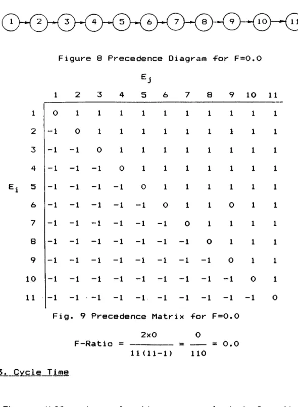
F = 0.0 - which provides a completely strict set of ordering relationships between the work elements. For

F = 0 . 0 , t h e p r e c e d e n c e d i a g r a m a n d t h e p r e c e d e n c e m a t r i x c a n b e s e e n i n F i g u r e 8 a n d 9 ^ r e s p e c t i v e l y .

Figure 8 Precedence Diagram -for F=0.0

Ei 1 2 3 4 5 6 7 8 9 10 1 1 1 0 1 1 1 1 1 1 1 1 1 1 2 -1 0 1 1 1 1 1 1 1 1 1 3 -1 -1 0 1 1 1 1 1 1 1 1 4 -1 -1 -1 0 1 1 1 1 1 1 1 5 -1 -1 -1 -1 0 1 1 1 1 1 1 6 -1 -1 -1 -1 -1 0 1 1 0 1 1 7 -1 -1 -1 -1 -1 -1 0 1 1 1 1 8 -1 -1 -1 -1 -1 -1 -1 0 1 1 1 9 -1 -1 -1 -1 -1 -1 -1 -1 0 1 1 10 -1 -1 -1 -1 -1 -1 -1 -1 -1 0 1 11 -1 -1 -1 -1 -1 -1 -1 -1 -1 -1 0

Fig. 9 Precedence Matrix -For F=0.0

2x0 0

F-Ratio =

1 1

11

1

= 0 . 0

4.1.3._Cycle Time

Three di-f-Ferent cycle time are selected for the research. These are:

C = 10, C = 20, C = 30 time units Cycle time are selected arbitrarily.

Work element times were assumed to be uniformly distributed between 0 and the cycle times (C).

Every combination of the cycle time and the F-ratios are tested with 4 selected heuristic methods, each for five times (5 replicates). The experimental design of the problem can be seen in Figure 10.

4j_l_j^4_._Worj<_Ej[ement_ Cl = 10 FI = 1., 0 C2 = 20 F2 = 0.,418 C3 = 30 F3 = 0,. 0

Fi , Cj

Figure 10. The Experimental Design

Total number of observations = # of cycle times x # of F-ratios X tt of heuristics x # replicates

= 3 x 3 x 4 x 5 = 1 8 0

4.2. PERFORMANCE MEASURE OF THE SOLUTION EFFICIENCY

As the cycle time is -fixed and given, the efficiency of a line balance is indicated by the total idle time in the assembly line. The performance measure used for solution efficiency is the commonly used Balance Delay or Imbalance Ratio which is defined by formula 2.1.6.1. in percentages.

4.3. SELECTED HEURISTIC PROCEDURES

Selected Heuristic Assembly Line Balancing Procedures are as follows;

- Heuristic method developed by W.B. Helgeson and D.P. Birnie (10)

- Heuristic method developed by M. Kilbridge and L. Wester (16)

- Heuristic method of number of Immediate followers - Heuristic method of number of followers

These heuristic methods will be explained in Chapter 5 in more detail.

CHAPTER V

5. ANALYSIS OF THE SELECTED METHODS AND SAMPLE SOLUTIONS

5.1. HEURISTIC METHOD DEVELOPED BY M. KILBRID6E AND L. WESTER

This method is one o-F the applicable methods in manufacturing plants where computers are not available. It requires some analysis of the problem data and does not need any sophisticated mathematical analysis. Simple arithmetic is sufficient for its application.

Method!

The objective of the method is the minimization of the balance delay and the selection of the line balance which meets this criterion.

For a perfect balance, the condition given below should be satisfied: m N X C - E t. = 0, i = l ^ that is N = E ti (5.1.1.)

Steps of the method are as follows: a) Determination of C and N.

To determine cycle times for which N is an integer Et^ will be written as a product of prime numbers and the cycle

time values are computed taking into consideration the possible range.

b) The precedence diagram is established such that the assembly progresses from left to right, each element being as far left as possible at the start of the procedure. In that diagram, elements in each vertical column are mutually independent and therefore can be permitted among themselves in any work sequence without violating restrictions on precedence relations. The second property is that elements can be moved laterally from their columns to right columns without disturbing the precedence restrictions.

c) Construction of a table containing detailed information about each element taken from the precedence diagram.

d) Assignment of work elements to stations. The assignment is made using the above mentioned table by rearranging work elements in a proper sequence in stations such that the station times will be equal to the selected cycle time. If there are two or more available elements, the one which has the biggest time will be preferred. In order to prevent the idle time, the permutation of work elements between columns should be arranged. For a particular C, if all the work elements can be fitted into the N work stations, perfect balance is attained. Otherwise the number of work stations is increased by the least integer required to achieve the

balance. In this case the balance is not perfect. For sample solution see Appendix B.

5.2. HEURISTIC METHOD BY U . B HELGESON AMD D . . BIRNIE

This method is also called "Ranked Positional Weight Technique". It is a simple and rapid, but approximate, method which has been shown to provide acceptably good solutions more quickly than many of the alternative methods. It is capable of dealing with precedence constrai nts.

M e t h g d _ L

Positional weight of work element is the sum of the element times of all the work elements which are following that work element in the precedence diagram plus its elemental time. Thus, it is a measure of the size of an element and its position in the precedence diagram.

The method can be summarized as follows;

a) Construction of precedence matrix and calculations of positional weights.

b) Ordering of work elements in the descending order of their positional weights.

c) Assignment of work elements to stations in the order determined in the second step. If an element takes longer than the remaining station time (unassigned time for the station) or if it violates precedence requirements, it will

be skipped and the next element will be tried. When the station time is completely used, then the remaining elements will be assigned to a new station. The elements which are skipped will be assigned in respective order to the new station. The process will be repeated until all the work elements are assigned. For sample solution see Appendix B.

5.3. HEURISTIC METHOD OF IMMEDIATE FOLLOWERS:

In this procedure, work elements are assigned according to the number of their immediate followers. The procedure can be summarized as follows:

a) Order elements in the descending order of the number of their immediate followers

b) Assign elements to stations by giving priority to the ones which has the most immediate followers. If there are two or more work elements which have the same number of immediate followers, the one which has the biggest element time should be selected.

Following constraints should be satisfied: - the determined cycle time should not be exceeded. ~ the precedence relationships should not be violated. For sample solution see Appendix B.

In this procedure, work elements are assigned according to their number of followers. The procedure can be summarized as follows;

5.4. H E U R I S T I C M E T H O D OF N U M B E R OF F O L L O W E R S :

a) Order elements in the descending order of the number of their followers in the precedence diagram.

b) Assign elements to stations by giving priority to the ones which has the most number of followers. If there are two or more work elements which have the same number of followers, the one which has the biggest element time should be selected.

The constraints which are mentioned in previous heuristic should be satisfied. For sample solution see Appendix B.

CHAPTER VI

EXPERIMENTAL RESULTS AND EVALUATION AMONG METHODS

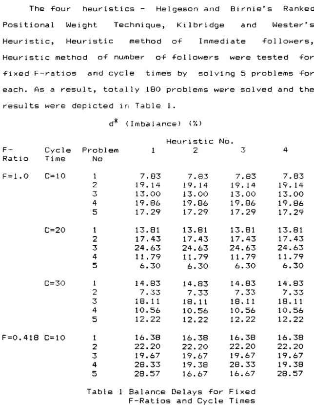
The -four heuristics - Helgeson and Birnie's Ranked Positional Weight Technique, Kilbridge and Wester's Heuristic, Heuristic method of Immediate followers, Heuristic method of number of followers were tested for fixed F-ratios and cycle times by solving 5 problems for each. As a result, totally 180 problems were solved and the results were dep i cted in Table 1 .

d* (Imbalance) (’/.) Heur i st i c No. F- Cycle Problem 1 2 3 4 Rat i o T i me No F=1.0 C=10 1 7.83 7.83 7.83 7.83 2 19.14 19.14 19.14 19. 14 3 13.00 13.00 13.00 13.00 4 19.86 19.86 19.86 19.86 5 17.29 17.29 17.29 17.29 C=20 1 13.81 13.81 13.81 13.81 2 17.43 17.43 17.43 17.43 3 24.63 24.63 24.63 24.63 4 11.79 11.79 11.79 11.79 5 6.30 6.30 6.30 6.30 C=30 1 14.83 14.83 14.83 14.83 2 7.33 7.33 7.33 7.33 3 18. 1 1 18. 1 1 18. 11 18.11 4 10.56 10.56 10.56 10.56 5 12.22 12.22 12.22 12.22 F=0.418 C=10 1 16.38 16.38 16.38 16.38 2 22.20 22.20 22.20 22.20 3 19.67 19.67 19.67 19.67 4 28.33 19.38 28.33 19.38 5 28.57 16.67 16.67 28.57

Table 1 Balance Delays for Fixed F-Ratios and Cycle Times

C = 20 C=30 F=0.0 C=10 C=20 C=30

1

1

F-Ratios and Cycle Times Abbreviations of the heuristics are as follows,

Heuristic #1 - Heuristic method developed by W.B. Helgeson and D. P. Birnie

Heuristic #2 - Heuristic method developed by M.Kilbridge and L. Wester

Heuristic #3 - Heuristic method of Immediate Followers Heuristic #4 - Heuristic method of Number of Followers

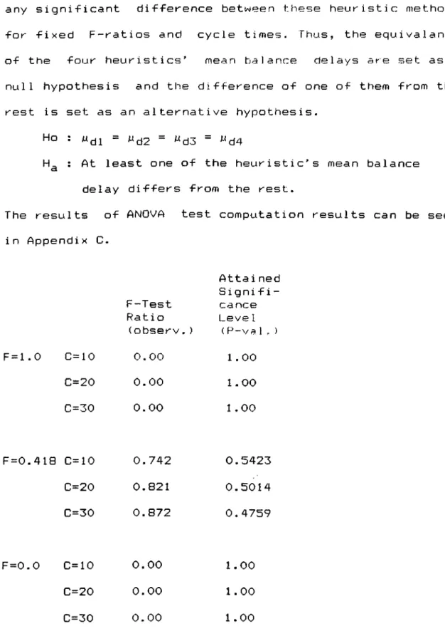
These results were statistically analyzed by one way analysis of variance (ANOVA) method for the four heuristic procedures. ANOVA method is used to examine if there are

any significant difference between these heuristic methods for fixed F-ratios and cycle times. Thus, the equ.ivalance of the four heuristics' mean balance delays are set as a null hypothesis and the difference of one of them from the rest is set as an alternative hypothesis.

Ho : “ ^*d4

: At least one of the heuristic's mean balance delay differs from the rest.

The results of ANOVA test computation results can be seen i n Append!x C . Atta i ned Signifi-F-T est Ratio (observ.) canee Leve 1 (P-vaI.

F = 1.0

C=10

1.00

C=20

0.00

1.00

C=30

0.00

1.00

F = 0 .4 ia C=10

0.742

0.5423

C=20

0.821

0.5014

C=30

0.872

0.4759

C=10

0.00

1.00

C=20

0.00

1.00

C=30

0.00

1.00

Table 2 Computation Results of ANOVA

As it can be seen from Table 2, for F-ratio=1.0 and for all C levels, the F-Test Ratio calculated for the heuristics is equal to zero and p -value equal to 1. From the table, we can reject or accept the null hypothesis either by looking at value or by looking at p-value. The observed F-test ratio is so small and p-value is so big, so we can conclude that there is insufficient evidence to reject the null hypothesis. Thus we can conclude that mean balance delays of the heuristics' do not significant 1y differ from each other.

For F=0.418 and for all cycle times, p-value is so big, so it can be concluded that mean balance delay of the 4 heuristics do not significantly differ from each other.

For F=0.0 and for all cycle times, p-value is equal to 1, so, we can conclude that there is no difference between the mean balance delays of the

heuristics"-As a result for 11 element assembly line, choosen heuristics do not significantly differ from each other and it can not be concluded that one of them gives better results than the others for 11-element Assembly Line Balancing Problem.

CHAPTER Vi I 7. CONCLUSION

In many industries such as home appliances, automobiles the product is assembled on a continuous conveyor line. The elemental task making up the assembly operation must be assigned to work stations along the line. The assignment oF a finite number of work elements to an ordered sequence of stations, sucii that the precedence relations are satisfied and the total idle time is minimized, is often called the “Assembly Line Balancing

Problem“-The assignment of work elements to stations with some improved trial and error methods is often called Heuristic Procedures- In this research, idle time or balance delay for the line was tried to be minimized for four different heuristic procedures for fixed F~ratios (strength of the partial ordering) and cycle times- Totally 180 problems were solved to make comparisons arnniK,i Uiem.

The results of the experiments show that there is no significant difference between the four selected heuristics in terms of solution efficiency. On the other hand, increase of the task size may change these results and

may cause at least one of the heuristics to dominate the others

-It was observed that as the F-ratio (Flexibility- Ratio) decreases the partial ordering becomes ’'strong'* and does not permit work elements to be assigned in many different ways. In other words, permutabi1ity between work element decreases and vice versa. It is also observed that, as the work element times gets smaller, line balancing is achieved in less number of stations.

It is expected that Kilbridge and Wester's Heuristic will dominate the other heuristics because ot permutabi1ity of work elements inside of the column and laterally movement between columns especially for large task sizes and large cycle times when one station crosses several columns.

The experiments were done under the conditions where F-ratio and cycle times were kept fixed and only heuristics were changed. Experimentation could be performed on a wider variety of line balancing problems. Experimental designs which considers more interactions of the F-ratios, cycle times, heuristic methods and the task size will increase the required observations and cost of obtaining them. Thus, this study will be a starting point for future studies which will need to cover more variable interactions and task sizes with the addition of computer programs and simulation packages.

The Pre cedence Diagram

1. _Purpose;

The precedence diagram is used to convert an actual assembly situation into a schematic diagram which is help-Ful in assembly line balancing studies.

2. _Construction of Precedence diagrams

2.1 Required data for construction of Precedence diagrams

a) Operation lists-time standards:

Lists o-F the assembly work elements and the correspond!ng performance times should be procured. The work elements should be those called "minimum rational work elements", defined as indivisible elements of work beyond which assembly work cannot be rationally divided. The elements in the list should be numbered for identification purposes.

b) Schematic Layout of the line.

This Layout should show the main and auxiliary lines, fixed facilities and storage spaces.

A P P E N D I X A

2.2 Notation used in Precedence diagrams:

In -figure Aj^ an example for F^recedence diagrams is given. The numbers within the circles are the element identification numbers whereas those outside the circles are the time durations corresponding the work elements. The lines and arrows between the circles indicate precedence relationships.

For the représentâtion of positional restrictions on precedence diagrams, letter codes, color or geometric symbols can be used. -Positional restrictions are restrictions imposed by the position of the worker and the product for the performance of assembly operations. Example; A work element which must be performed by an operator working in front of the line with the back of the product facing

him.-11 12 III 8 IV VI VII 10 3 6

Generally letter codes are used when the number o-F positional restrictions are large.

For the représentâtion of fixed facility restrictions on the diagram asterisks are placed next to the circles. Such restricted elements are also plotted on the shematic

layout to show the location where they should be performed, and entered into a data sheet with the explanatory

information and remarks. The asterisk warns the diagram user about the fixed facility restrictions. An example of a fixed facility restriction could be : The work element 6 must be performed within 10 feet the start of the

line-2.3 Co nstruction technique;

Elements that should be performed first on the assembly line, such as the placement of a major component (a frame, a chassis) should be assigned to the first column in the diagram. Then, elements that need to be preceded by the elements entered in the first column will be assigned in the second column. This will continue to ward the right until the assignment of all the work elements are completed. The connecting lines which show precedence relationships are drawn during the assignment of work elements to columns. The coding for positional restrictions

and the asterisks for the fixed facility restrictions should also be added during the construction of the diagram. For the fixed facility restrictions the necessary information should be entered into the data sheet and the schematic Layout or drawing.

For Simplifying the construction of precedence diagrams, it is advisable to think in terms of groups of elements. The groups will be formed by work elements which must be performed before a certain point on the line, or work elements which should precede the assembly of a major component. When the first element of the group is entered into the diagram the following elements will be automatically assigned to the succeeding columns.

3^_Advantages__tq_be__fl^ined frqm__the__use__of__Precedence d iagram

1“ Visualization of the assembly operations and the precedence relationship.

2“ Clearer understand!ng of the existing assembly l i n e .

3- Simplicity which permit new personnel to balance the assembly lines by the use of previously collected data and the precedence diagram.

SAMPLE SOLUTION OF THE SELECTED HEURISTIC METHODS

The sample problem is solved -For each heuristic method with fixed parameters given below,

F-ratio = 0.418, Cycle time = 10

The precedence diagram and the precedence matrix of the sample problem can be seen in Figure 6 and 7 respect i v e 1y

-1. SAMPLE SOLUTION FOR THE HEURISTIC METHOD OF M. KILBRIDGE AND L. WESTER A P P E N D I X B Element Identification No Element T ime < t ^) 1 2.6 2 9. 1 3 1.0 4 9.0 5 6.6 6 9.0 7 2.2 S 7.2 9 7.6 10 9.4 11 3.2 E t^ = 66.9 3 9

a) Determination of C and N.

C is given and equal to 10. For the determination of N (number of stations), total work content time should be divided to C. As a result,

E t^ 66.9

N = --- = ---= 6.69

C 10

This number is not an integer so perfect balance is not possible. The number is rounded to 7. There are at

least 7 or more stations required for balancing the line.

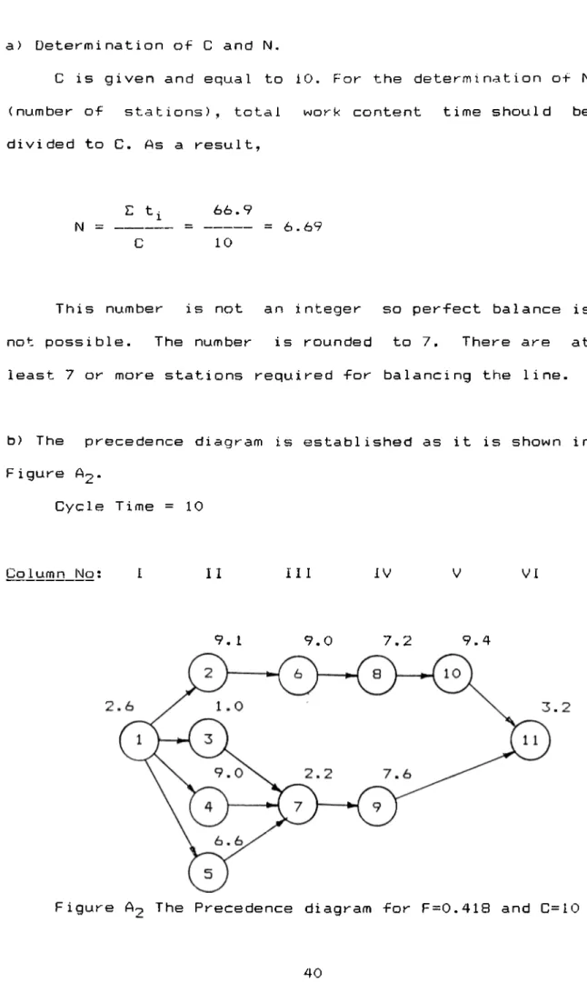
b) The precedence diagram is established as it is shown in Figure A

2

Cycle Time = 10

Column No: I I I I 11 IV V VI

9. 1 9.0 7.2 9.4

Figure The Precedence diagram for F=0.418 and C=10

c) The tabular representation of Precedence Diagram is given below.

Column Element Element Cumulative

Number Identification Remarks Time _____Time

I 1 2.6 2.6 11 2 9. 1 3 <W.7,9) --- > I I I 1.0 4 (W.7,9) --- > III 9.0 5 (W.7,9) --- > III 6.6 28.3 III 6 9.0 7 (W.9) --- > IV 2.2 39.5 IV 8 7.2 9 --- > V 7.6 54.3 V 10 9.4 63.7 VI 11 3.2 66.9 4 1

d) A s s i g n m e n t o-F w o r k e l e m e n t s t o t h e s t a t i o n s . ( F o r C = 1 0 ) Element Identification No Element T ime Cumulative Station

T ime Station No,

1 2.6 5 6.6 9.2 1 2 9. 1 9. 1 2 4 9.0 3 1.0 10.0 3 6 9.0 9.0 4 8 7.2 7 2.2 9.4 5 10 9.4 9.4 6 9 7.6 7.6 7 11 3.2 3.2 8

As it can be seen from the table there are eight stations required for balancing the line. Again, this balance is not a perfect balance because of the idle time.

2. SAMPLE SOLUTION FOR THE HEURISTIC METHOD OF W.B. HELGESON AND D.P.BIRNIE

The precedence diagram for F=o.418 and C=10 is given in Figure 6. The steps for the procedure are as follows;

a) The precedence matrix is represented in Figure 7.

For element 1 positional weight can be calculated as -Fol lows; iNiork element no 1 2 3 4 5 6 7 8 9 10 11 1 0 1 1 1 1 1 1 1 1 1 1 work element 2.6 9.1 1.0 9.0 6.6 9.0 2.2 7.2 7.6 9.4 3.2 time Positional weight = 2-6 + 9. 1 + 1.0 + 9. 0 + 6.6 + 9.0 + 2.2 + 7. 2 + 7.6 + 9.4 + 3.2 = 66.9

b) Ordering o-f work elements according to their positional weight. Ranked Positional Weight Work Element No Work Element T ime Immediate Predecessor No 66.9 1 2.6 37.9 2 9. 1 1 28.8 6 6.6 2 22.0 4 9.0 1 19.8 8 7.2 6 19.6 5 6.6 1 14.0 3 1.0 1 13.0 7 2.2 3,4,5 12.6 10 9.4 8 10.8 9 7.6 7 3.2 11 3.2 9, 10 4 3

c) A s s i g n m e n t o f t h e w o r k e l e m e n t s t o s t a t i o n s ( f o r C = 1 0 ) E 1ement I dent ification No E 1ement T i me Camu1 a t i ve Stat ion T i me Station No. 1 2.6 5 6.6 9.2 1 2 9. 1 9. 1 2 6 9.0 3 1.0 10.0 3 4 9.0 9.0 4 8 7.2 7 2.2 9.4 5 10 9.4 9.4 6 9 7.6 7.6 7 1 1 3.2 3.2 8

As it can be seen from the table, there are 8 stations required for the balance of the line.

3- SAMPLE SOLUTION FOR THE HEURISTIC METHOD BY IMMEDIATE FOLLOWERS:

The precedence diagram for F=0.418 and 0=10 is given in Figure 6. The steps of the sample solution are as follows:

a) R a n k w o r k e l e m e n t s a c c o r d i n g t o t h e i r i m m e d i a t e f o l l o w e r s Element Identification No Immediate Followers Immediate Predecessor No

1

1

1

1

1

1

1

1

1

1

b) Assignment of elements to Element Identification Element No Time the stations Cumulative Station T ime . (For C=10) Station No. 1 2.6 5 6.6 9.2 1 2 9. 1 9. 1 2 6 9.0 3 1.0 10.0 3 4 9.0 9.0 4 8 7.2 7 2.2 9.4 5 10 9.4 9.4 6 9 7.6 7.6 7 1 1 3.2 3.2 8

4. SAMPLE SOLUTION FOR THE HEURISTIC METHOD BY NUMBER OF FOLLOWERS:

The precedence! diagram for F=0.418 and C=10 is given i n Figure 6. The steps of the sample solution are as ■Follows;

a) R a n k w o r k e l e m e n t s a c c o r d i n g t o t h e i r n u m b e r o f •Fo 11 o w e r s .

Element

I dent i-Fi cat i on # o+' -Followers Element

No T ime Immediate Predecessor No 1 2 3 4 5 6 7 8 9 10 1 I

10

1

1

1

,

b) A s s i g n m e n t o f e l e m e n t s t o t h e s t a t i o n s ( F o r C = 1 0 ) Element Identification No Element T ime Cumulative Station T i me Station No, 1 2.6 5 6.6 9.2 1 2 9. 1 9. 1 2 4 9.0 3 1.0 10.0 3 6 9.0 9.0 4 8 7.2 7 2.2 9.4 5 10 9.4 9.4 6 9 7.6 7.6 7 1 1 3.2 3.2 8 4 8

APPENDIX C

ANQVA TEST COMPUTATION RESULTS

■- ANALYSIS OF VAPIAMCF

HEADER DATA FOR: B:DD

LABEL;

NUMEIER OF CASES: 180

NUMBER OF VARIABLES: 1

ONE-WAY ANOVA

F = 1.0 C=10 l-H&B 2-K&W 3-IM. F O L . 4-it FOL

GROUP

MEAN

N

1

15.424

5

2

15.424

5

3

15.424

5

4

15.424

5

GRAND MEAN

15.424

20

VARIABLE

1: (%)

SOURCE

SUM OF SQUARES

D .F . MEAN SQUARE

BETWEEN

.000

.000

WITHIN

402.0.53

16

25,128

TOTAL

402.053

19

F RATIO

.000

PROB.

ANALYSIS OF VARIANCE

---HEADER DATA FOR: B:DD

LABEL: D*

NUMBER OF CASES; 180

NUMBER OF VARIABLES: 1

ONE-WAY ANOVA

F-1.0 C=20 l-H&B 2-K&W 3-IM. FOL. 4-# FOL

GROUP

MEAN

N

1

14.790

5

2

14.790

5

3

14.790

5

4

14.790

5

GRAND MEAN

14.790

20

VARIABLE 1: (%)

SOURCE

SUM OF SQUARES

D.F.

MEAN SQUARE

F RATIO

PROB .

BETWEEN

.000

3

.000

.000

1.0000

WITHIN

743.069

16

46.442

TOTAL

743.069

19

■- ANALYSIS OF VARIANCE

--HEADER DATA FOR: E:DD

LABEL: D^f

NUMBER OF CASES: 180

NUMBER OF VARIABLES: 1

ONE-WAY ANOVA

F=1.0 C=30 l-H&B 2-K&W 3-IM. FOL. 4-# FOL

GROUP

MEAN

N

1

12.610

5

2

12.610

5

3

12.610

5

4

12.610

5

GRAND MEAN

12.610

20

VARIABLE 1: (%)

SOURCE

SUM OF SQUARES

D.F.

MEAN SQUARE

F RATIO

PROB.

BETWEEN

.000

3

.000

.000

1.0000

WITHIN

269.702

16

16.856

TOTAL

269.702

19

ANALYSIS OF VABIANCE

HEADER DATA FOR: B:DD

LABEL: Dt

NUMBER OF CASES: 180

NUMBER OF VARIABLES: 1

ONE-WAY ANOVA

F = 0..418 C=10 l-H&B 2-K&W 3-IM. FOL.

4-GROUP

MEAN

N

1

23.030

5

2

18.860

5

3

20.650

5

4

21.240

5

GRAND MEAN

20.945

20

VARIABLE

1: (%)

SOURCE

SUM OF SQUARES

D.F. MEAN SQUARE

BETWEEN

44.343

3

14.781

WITHIN

318.624

16

19.914

TOTAL

362.967

19

F RATIO

.742

PROB .

. 5423

--- ANALYSIS OF VARIANCE

HEADER DATA FOR: B:DD

NUMBER OF CASES: 180

NUMBER OF VARIABLES: 1

LABEL: D*

ONE-WAY ANOVA

F = 0,.418 C-20 l-H&B 2 -K&W 3-IM. FOL.

4-GROUP

MEAN

N

1

15.561

5

2

15.561

5

3

17.978

5

4

15.561

5

GRAND MEAN

16.165

20

VARIABLE

1: (%)

SOURCE

SUM OF SQUARES

D.F. MEAN SQUARE

BETWEEN

21.907

3

7.302

WITHIN

142.382

16

8.899

TOTAL

164.290

19

d^(%)

F RATIO

.821

PROB.

. 5014

ANALYSIS OF VARIANCE

-HEADER DATA FOR; B:DD

NUMBER OF CASES: 180

NUMBER OF VARIABLES:

LABEL: D-t.

ONE-WAY ANOVA

F = 0,.418 C:=30 l-H&B 2-Ki5tW 3-IM. FOL.

4-GROUP

MEAN

N

1

19.402

5

2

19.402

5

3

19.402

5

4

22.147

5

GRAND MEAN

20.088

20

VARIABLE

1·· (%)

SOURCE

SUM OF SQUARES

D .F . MEAN SQUARE

BETWEEN

28.252

3

9.417

WITHIN

172.713

16

10.795

TOTAL

200.965

19

RATIO

.872

PROB.

.4759