Evidence for 'Flight to Quality' hypothesis within an inflation uncertainty modelling

EVIDENCE FOR ‘FLIGHT TO QUALITY’

HYPOTHESIS WITHIN

AN INFLATION UNCERTAINTY MODELLING

A Master’s Thesis

by

BÜLENT GÜLER

Department of Economics

Bilkent University

Ankara

July 2003

EVIDENCE FOR ‘FLIGHT TO QUALITY’ HY

POTHESIS WITHIN AN INFLATION

UNCERTAINTY MODELLING

EVIDENCE FOR ‘FLIGHT TO QUALITY’

HYPOTHESIS WITHIN

AN INFLATION UNCERTAINTY MODELLING

The Institute of Economics and Social Sciences

of

Bilkent University

by

BÜLENT GÜLER

In Partial Fulfilment of the Requirements for the Degree of

MASTER OF ARTS IN ECONOMICS

in

DEPARTMENT OF ECONOMICS

BILKENT UNIVERSITY

ANKARA

July 2003

EVIDENCE FOR ‘FLIGHT TO QUALITY’ HY

POTHESIS WITHIN AN INFLATION

UNCERTAINTY MODELLING

ABSTRACT

EVIDENCE FOR ‘FLIGHT TO QUALITY’ HYPOTHESIS WITHIN

AN INFLATION UNCERTAINTY MODELLING

Güler, Bülent

M.A., Department of Economics

Supervisor: Asst. Prof. Ümit Özlale

July 2003

There is a great literature devoted to link between inflation uncertainty and interest

rates. However, there are opposing findings about the relationship between inflation

uncertainty and interest rates. Some of the studies find a positive correlation between them,

while some of them find a negative correlation. In this paper, we analyzed the link between

inflation uncertainty and spreads among riskier and safer bonds within a model of a

time-varying parameter model with an ARCH specification. We divided inflation uncertainty into

two parts, structural uncertainty and impulse uncertainty, as indicated in Evans (1991), firstly.

We estimated the relationship between these types of uncertainties and spreads among riskier

and safer bonds, using USA data.

The results indicate us that both structural and impulse uncertainties have significant

relationship with spreads between corporate bonds, the riskier bonds, and treasury bills, the

safer bonds. Especially having a positive effect of impulse uncertainty on spreads shows an

important evidence for ‘Flight to Quality’ hypothesis.

Keywords: ‘Flight to Quality’, structural uncertainty, impulse uncertainty, spread, Kalman

Filter

ÖZET

‘KALİTEYE KAÇIŞ’ HİPOTEZİNE ENFLASYON BELİRSİZLİĞİ

MODELLEMESİYLE KANIT

Güler, Bülent

Master, Ekonomi Bölümü

Tez Yöneticisi: Yrd. Doç. Dr. Ümit Özlale

Temmuz 2003

Enflasyon belirsizliği ve faiz oranları arasındaki ilişkiyi inceleyen geniş bir literatür

mevcuttur. Fakat, bu ilişki konusunda karşıt buluşlar bulunmaktadır. Bazı çalışmalar,

enflasyon belirsizliği ve faiz oranları arasında pozitif bir ilişkinin varlığını gösterirken bazı

çalışmalar da negatif bir ilişkiden söz etmektedirler. Bunların ötesinde, biz bu tezde, ARCH

modellemesiyle birlikte zaman içerisinde değişen parametre modeli kullanarak enflasyon

belirsizliği ile riskli ve güvenli bonolar arasındaki marj ilişkisini inceledik. Öncelikle

enflasyon belirsizliğini, Evans (1991)’de belirtildiği gibi, “yapısal belirsizlik” ve “ani

belirsizlik” diye iki kısma böldük. Ardından da A.B.D. verilerini kullanarak, bu iki

belirsizliğin riskli ve güvenilir bono marjı üzerindeki etkilerini inceledik.

Sonuçta, “yapısal belirsizlik” ve “ani belirsizlik” in şirket tahvilleri, riskli tür bonolar, ile

hazine bonoları, güvenilir tür bonolar, arasındaki marj üzerinde anlamlı bir etkisinin olduğunu

bulduk. Özellikle “ani belirsizlik” in marjlar üzerinde pozitif bir etkisinin olması ‘Kaliteye

Kaçış’ hipotezine önemli bir kanıt oluşturmaktadır.

Anahtar Kelimeler: ‘Kaliteye Kaçış’ hipotezi, yapısal belirsizlik, ani belirsizlik, marj, Kalman

Filtresi.

I certify that I have read this thesis and have found that it is fully adequate, in scope and in

quality, as a thesis for the degree of Master of Economics.

---

(Title and Name)

Supervisor

I certify that I have read this thesis and have found that it is fully adequate, in scope and in

quality, as a thesis for the degree of Master of Economics.

---

(Title and Name)

Examining Committee Member

I certify that I have read this thesis and have found that it is fully adequate, in scope and in

quality, as a thesis for the degree of Master of Economics.

---

(Title and Name)

Examining Committee Member

Approval of the Institute of Economics and Social Sciences

---

(Title and Name)

Director

TABLE OF CONTENTS

ABSTRACT ... iii

ÖZET ... iv

ACKNOWLEDGMENTS ... v

TABLE OF CONTENTS ... vi

LIST OF TABLES ……… vii

LIST OF FIGURES ………... viii

1 INTRODUCTION ...………. 1

1.1

Literature on ‘Flight to Quality’ Hypothesis...……. 1

2 THE MODEL ...………….. 6

2.1 Modeling Inflation Uncertainty ...…….. 6

2.2 Justification of the Model ...…… 10

3 RESULTS ...……… 11

3.1 Data Set...……… 11

3.2 Estimation Results ...………... 13

3.3 Testing the “Flight to Quality” Hypothesis...….. 16

3.4 Robustness of Estimation Results...………. 18

4 CONCLUSION ...……….... 19

BIBLIOGRAPHY ...…… 20

APPENDICES

A. MATLAB CODES FOR THE MODEL...…… 24

LIST OF TABLES

1.

Estimation Results for Effects of Uncertainties on Various Bonds...15

LIST OF FIGURES

1.

The behavior of monthly USA inflation from 1953:04 to 2002:11 …... 12

2.

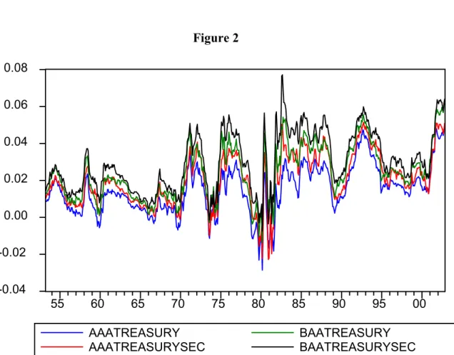
The behavior of various interest rate spreads with 3-month maturity ……… 12

3.

The behaviour of structural uncertainty from 1953:04 to 2002:11 ... 14

4.

The behaviour of impulse uncertainty from 1953:04 to 2002:11 ……….. 14

5.

Jointly behaviors of corporate bonds, structural uncertainty and

impulse uncertainty ……….. 17

6.

Jointly behaviours of treasury bill, structural uncertainty and

1 Introduction

In all types of economies, permanent and/or temporary modifications, adjustments or

variations can change the important dynamics in the economy. ‘Flight to Quality’

hypothesis emerges as one of these consequences of changes or variations in

monetary policy on real economic dynamics. This hypothesis proposes that sudden

shocks to the economy, temporary or permanent, will lead investors to escape from

“bad” investment options to “good” investment options. These two options vary by

the type of investment. It can be “low quality” versus “high quality”, or “short-term”

versus “long-term”, as well as “low-return” versus “high-return”, or “riskier” versus

“safer” etc.

1.1 Literature

on

‘Flight to Quality’ Hypothesis

There is an extensive literature devoted to the ‘Flight to Quality’ effect in terms of

lender-borrower relationship. Bernanke and Gertler (1989) shows in a model, where

firms are financed by Townsend-style (1979) optimal debt contracts which allows

converting i.i.d shocks into autoregressive movements in output

, that when

prospective agency costs of lending (in the form of bankruptcy risks) increase,

lenders reduce the amount of credit extended to firms that require monitoring and

invest a greater share of their savings in the safe alternative

_{. Bernanke and Gertler}

(1990) and Calomiris and Hubbard (1990) analyze a similar result such that a

reallocation of credit in downturns from low-net-worth to high-net-worth borrowers

occurs when costs of lending increase. Moreover Gertler (1992) exhibits qualitatively

similar results to Bernanke and Gertler (1989) framework that emerge when

1 _{Aghion and Bolton (1993) gives an extended analysis of dynamics in a related model} 2 _{Williamson (1989) finds a similar result of Bernanke and Gertler (1989).}

borrowers and lenders contract for multiple periods. He finds that with multi-period

relationships, expected future profits of the borrower can partially substitute for

internal finance in reducing agency costs. Since an increase in the safe real interest

rate reduces the present value of expected profits, Gertler’s result reinforces the point

that higher interest rates worsen the agency problem.

‘Financial accelerator’

theory predicts a differential effect of an economic

downturn on borrowers who are subject to severe agency problems in credit markets

and borrowers who don’t face serious agency problems; the difference arises because

declines in net worth raise the agency costs of lending to the former but not the latter.

Therefore, if financial accelerator is operative, at the beginning of a recession we

should see a decline in the share of credit flowing to those borrowers more subject to

agency costs (the flight to quality). As a result of their greater cost or difficulty in

obtaining credit, these borrowers should reduce spending and production earlier and

more sharply than do borrowers with greater access to credit markets. The

consequences of monetary policy in generating a ‘Flight to Quality’ effect have also

been widely studied. In this manner Bernanke and Blinder (1988), and Kashyap and

Stein (1994) state that recessions following a tightening of monetary policy involve

‘Flight to Quality’, because of the adverse effect of increased interest rates on

balance sheets and because monetary tightening may reduce flows of credit through

the banking system. Kashyap, Stein, and Wilcox (1993), Gertler and Gilchist (1993),

and Oliner and Rudebusch (1993) show that after tightening of monetary policy there

is a sharp increase in commercial paper issuance, while bank loans are flat, which is

consistent with ‘Flight to Quality’ hypothesis

.

3 _{It means the amplification of initial shocks brought about by changes in credit-market conditions.} 4 _{Kashyap, Stein, and Wilcox (1993) explains this result by the limitation of the supply of bank credits} by the tightening of monetary policy, whereas Gertler and Gilchist (1993), and Oliner and Rudebusch

Lang and Nakamura (1992), on the other hand, finds that the share of the bank loans

made above prime (i.e. loans to riskier or harder-to-monitor borrowers) drops in

recessions. Additionally Morgan (1993) demonstrates that, following a tightening of

monetary policy, firms without previously established lines of credit receive a

smaller share of bank loans

. Finally, in the favour of the ‘Flight to Quality’

hypothesis, Corcoran (1992), and Carey, Browse, Rea, and Udell (1993) suggest that

private placements fall sharply relative to public bond issues during recessions and

tight-money periods.

1.2 Literature on Inflation Uncertainty

As a different strand, in recent years, there is a growing interest on the inflation

uncertainty, which affects real economic activities directly or indirectly. As

Berument, Kilinc, and Ozlale (2002) states in a society with a high degree of

inflation uncertainty, there will be serious errors in inflation forecasts, which will

mislead the investors, who plan their future activities in the light of these inflation

forecasts, by reducing the credibility of economic policies and causing high inflation

risk premium. There can be observed many studies on the analysis of the inflation

uncertainty over inflation, employment and output. Cukierman and Wachtel (1979),

Cukierman and Meltzer (1986), Ball and Cecchetti (1990), Ball (1992), Evans and

Wachtel (1993), and Holland (1993b and 1995) all find a positive relationship

between inflation uncertainty and inflation. Hafer (1986) and Holland (1986) observe

negative correlation between inflation uncertainty and employment. Friedman

(1977), Froyen and Waud (1987), and Holland (1988) report a negative relationship

between output and inflation uncertainty. Furthermore Berument, Kilinc, and Ozlale

5_{He also emphasizes that declines in noncommitment lending are highly correlated with increases in} the share of the membership of the National Federation of Independent Business reporting that credit has become harder to obtain.

(2003) analyses the effect of inflation uncertainty on the long-short term interest rate

spreads and finds a positive correlation between inflation uncertainty and the spread

between several types of interest rates and the overnight interbank interest, which is

the shortest term.

Routledge and Zin (2001) explores connection between uncertainty and liquidity.

Their investigation depends on the two common features of various crises

. Firstly,

times of crises are associated with a greater degree of uncertainty. Secondly, crises

are accompanied by a severe lack of liquidity. Following the various recent

international and domestic crises, liquidity disappeared. Bid-ask spreads increase,

people have difficulty executing trades for existing financial securities, and new

bond and equity offerings are postponed or canceled.

To explore the connection of uncertainty with liquidity, they specify a simple market

where a monopolist financial intermediary makes a market for a propriety derivative

security. The market-maker chooses bid and ask prices for the derivative, then,

conditional on trade in this market, chooses an optimal portfolio and consumption.

Within this framework, they find a positive relationship between bid-ask spread and

uncertainty, and hence, a negative correlation between uncertainty and liquidity.

However, there is a missing literature on the consequence of inflation uncertainty on

‘Flight to Quality’ hypothesis, in terms of escaping from riskier bonds to safer bonds.

We expect variations in the yields of interest rates due to the volatility in the market,

which causes uncertainty in decisions of agents. This fact can be seen by looking at

financial options. There are two kinds of financial options: A call gives its holder the

right but not the obligation to purchase a particular security at a given price (the

6 _{Russian debt crisis in August 1998, Mexico, Thailand, Indonesia, South Korea, and Brazil crises} during 1990s (analysed deeply in Summers (2000)), USA municipal bond crisis, various USA stock

strike price); a put confers the right but not the obligation to sell at the strike price.

This structure makes option prices very sensitive to market volatility.

In this paper we tried to connect the missing linkage between the inflation

uncertainty and ‘Flight to Quality’ hypothesis. For this purpose, we analyzed

relationship between spreads of risky-safer bonds and different types of inflation

uncertainty, as introduced by Evans (1991) and used in Berument (1999), and

Berument, et al (2002 and 2003), and tried to see whether there is a flight to quality

effect or not. As Evans (1991) introduced there may be an uncertainty about the

structure of the inflation process, which is originated from the conditional variance of

expected inflation and called “structural uncertainty”. Also, uncertainty may occur

due to the nature and magnitude of temporary shocks that hit the economy, which is

originated from the conditional variance of given inflation and named as “impulse

uncertainty”. We used a time-varying parameter model with an Autoregressive

Conditional Heteroscedasticity (ARCH) specification to measure the structural and

impulse uncertainties. Furthermore we regressed these uncertainties on the spread

between corporate bond (riskier bonds) and treasury bills (safer bonds) by using

Least Square Estimation (LSE) technique while impulse uncertainty is found to have

a positive effect on the interest rate spread, which is in favor of the ‘Flight to

Quality’ hypothesis, structural uncertainty seems to have a negative effect on the

spread.

The plan of this paper is as follows: Section 2 explains the model used to measure

two types of inflation uncertainty, structural uncertainty and impulse uncertainty and

the motivation of using such a model. Section 3 begins with the definition of the data

used in this paper and then demonstrates the estimation results for ‘Flight to Quality’

hypothesis, and as a final point, checks for the robustness of the results. Finally

Section 4 concludes the paper with a summary of the results.

2 The

Model

2.1 Modeling Inflation Uncertainty

In the literature several methods for measuring inflation uncertainty are proposed.

The first method is the survey-based approach, used by Hafer (1986), and Davis and

Kanago (1996). They find a negative correlation between inflation uncertainty and

real economic dynamics. However, as Bomberger (1996) states in his study, since

survey-based approach could just measure the disagreement, and moreover results of

the survey could be biased due to the fact that forecasters might try to avoid

deviating from the others’ forecasts, it cannot provide a true measure of inflation

uncertainty.

Furthermore, it is crucial to mention that variability and uncertainty are not identical.

Although a small volatility is observed in actual inflation ex post, agents may view

the future with a great amount of uncertainty due to having very little information.

On the other hand, there may be a great volatility in the behavior of inflation, but

agents may view future with a very small amount of uncertainty due to having a good

deal of advanced information. As a result, measuring inflation uncertainty depending

solely on the variability or simple variance of actual inflation may be misleading. To

avoid this problem, a second method that uses the conditional variance of

period-to-period inflation as the main source of the uncertainty, (generalized as ARCH model)

emerges to measure inflation uncertainty. In these types of models, changes in

variability in ex post inflation are equated with changes in uncertainty when the time

(1979), and Mullineaux (1980) use the cross-sectional variance of the inflation

forecasts, while Cukierman and Wachtel (1982) employs the mean squared error of

the inflation forecast. Finally, Holland (1986) takes the root mean squared error of

the inflation forecasts as a proxy for inflation uncertainty. All of these

above-mentioned models make use of ARCH specification. However, since a raise in the

conditional variance of next period’s inflation rate may be unrelated to the precision,

this method solely cannot capture all the economically relevant aspects of inflation

uncertainty.

Furthermore another method, the Kalman Filter approach, is an extended form of the

above method, and measures the uncertainty by estimating the time-varying

conditional variance of the parameter estimates of a variable.

In this study, as in Evans (1991), we used a time-varying parameter model with an

ARCH specification, by combining the last two methods emphasized above to

measure structural and impulse uncertainties.

Let

π

stands for the inflation rate between t and

t

+

1

. With an aid of ARCH

specification, the inflation uncertainty can be modeled as:

e

X

=

β

+

π

where

e

_t

₊

₁

~

N

(

0

,

h

t

)

(1)

V

=

β

+

β

where

V

~

N

(

0

,

Q

)

(2)

∑

∑

+

+

=

h

e

h

h

γ

φ

₍₃₎

where

_X

is a vector of explanatory variables for inflation, known at time t,

β

1 +

t

is

a vector of parameters,

_e

is the shock to inflation that cannot be forecasted with

information at time t, and

e

is normally distributed with a time-varying

conditional variance of

h , which indicates the changes in uncertainty of the future

inflation at time t and is specified as a linear function of current and past squared

forecast errors.

φ

and

γ

are the time-varying parameters of

h .

In this modeling, equations (1) and (3) represent a generic ARCH specification of

inflation. Nevertheless, they are not sufficient to capture some important feature of

the inflation process. As the dynamics of economy change over time, it is likely to

have significant variations in the structure of inflation, which causes

β

to vary over

time. This feature is obtained by equation (2), where

_V

is a vector of normally

distributed shocks to the parameter vector

β

1 +

t

with a homoskedastic covariance

matrix

Q . By this way, equations (1), (2), and (3) characterize a time-varying

autoregressive process with an ARCH specification for shocks to inflation. However,

now,

h becomes a poor estimate for inflation uncertainty. Suppose that, at time t, it

is announced that at time

t+1 the monetary policy will be changed. If the agents have

perfect information about the structure of inflation, then the expected rate of inflation

will be

E

π

=

X

β

, and the variance of inflation will be

h . On the other hand, if

the agents have poor information, then agents will expect the inflation to be

represented as

E

π

=

X

E

β

. Then, since

h ignores the variations from the true

value of

β

, it cannot represent the true value of the inflation uncertainty.

In order to see the effects of variations in the structure of inflation on uncertainty, we

should include the Kalman Filter equations (see Chow (1984) for details):

η

β

π

=

X

E

+

,

(4)

h

X

X

H

=

Ω

+

(5)

[

]

η

β

β

1

=

+

Ω

+

X

H

E

t

(6)

[

]

Q

=

I

−

Ω

X

H

X

Ω

+

Ω

(7)

where

Ω

stands for the conditional covariance matrix of

β

1 +

t

, which represents

the uncertainty about the structure of the inflation process. Since equation (4)

indicates that innovations in the inflation rate, which is denoted by

η

1 +

t

, may come

from both inflation shocks

e

and unanticipated changes in the structure of

inflation

_V

, the conditional variance of inflation

_H

depends upon both

_h

and

the conditional variance of

β

1 +

t t

X

, which is

_X

Ω

_X

, formulated in equation

(5). If there is not any uncertainty about the vector of parameters,

β

1 +

t

(

Ω

is

equal to the null matrix), then

_h

will entirely govern the conditional variation of

inflation. This means that the model covers the generic ARCH specification,

formulated by equations (1) and (3). Otherwise, if there is uncertainty about the

structure of inflation, then

h

will miscalculate the true conditional variance of

inflation,

_H

, since

Ω

>

0

t t t

t

X

X

. Equation (6) shows the innovations in updating

the estimates of

β

1 +

t

, which is used for forecasting the future inflation. Finally

equations (6) and (7) represent the updating of the conditional distribution of

β

1 +

t

al (2002), we can refer to inflation uncertainty associated with randomness in

β

as

“structural uncertainty”, which is denoted by

_X

Ω

_X

; while the uncertainty

associated with the randomness in “

e

” is called “impulse uncertainty” and

represented by the conditional variance of

e

, which is

h .

2.2 Justification of the Model

In this part we will explain the motivation for choosing a time-varying parameter

model with an ARCH specification in a detailed form. Especially we will clarify the

reason behind using both time-varying parameters and ARCH specification within a

single model. Evans (1991) gives two reasons for this fact:

… inflation shocks represent combinations of structural disturbances such as

productivity, money supply, and price shocks. Over time it is unlikely that the

actual or perceived frequency with which these structural disturbances occur

remains constant. For example, the variance of monetary shocks is likely to

be higher during periods of greater uncertainty about the future course of

monetary policy. Similarly, the variance of price shocks probably rises

around OPEC meetings.

The Lucas critique provides another reason. Since the inflation process

represents the result of a large number of price-setting decisions, shocks to

the aggregate price level must in part depend upon how individual price

setters respond to structural disturbances. For example, the pricing strategies

of individual firms will determine the aggregate effects of a given nominal

demand shock. Such pricing rules are subject to change. In particular the

analysis in Ball, Mankiw, and Romer (1988), Evans (1989), and others

suggest that the frequency of individual price changes should rise as the

economy moves toward regimes of higher inflation so that the aggregate price

level will respond more quickly to nominal shocks. Under these

circumstances, a prolonged increase in the rate of inflation will induce a rise

in the conditional variance of inflation independently of the perceived

frequency of nominal shocks.

The reasons indicated above suggest that time-varying model with an ARCH

specification captures the important features for the inflation process. Behavioral and

policy changes in the economy will both persuade ARCH effects and time variation

in the structure of inflation, which the above model already confines.

3 Results

3.1 Data

Set

We employ monthly USA data from 1953:04 to 2002:11. Since most of the studies

related to

‘Flight to Quality’ hypothesis and inflation uncertainty take United States

economy as the main observation, we will be able to compare our results with the

existing literature.

Monthly inflation of USA is obtained from CPI (Consumer Price Index) data

.

Structural uncertainty and impulse uncertainty are obtained using this inflation data

in the equations (1) to (6)

. Interest rates used in the spreads are the AAA type

corporate bond, treasury bill rate, BAA type corporate bond and secondary market

treasury bill rate

. All these interest rates have equivalent maturity, which is 3 month.

Interest rate spread is obtained by taking the difference between AAA type corporate

bond and treasury bill rate (AAA-treasury)

. Also for robustness of the results, the

spread is obtained by taking the difference between BAA type corporate bond and

secondary market treasury bill rate (BAA-treasurysec), BAA type corporate bond

and treasury bill rate (BAA-treasury), and finally, AAA type corporate bond and

second market treasury bill rate (AAA-treasurysec)

. Figure 2 shows the behavior

of spreads, and they are positive most of the time. Elton, Gruber, Agrawal, and Mann

(2001) suggests three possible reasons for this fact:

8 _{The Matlab codes for obtaining the structural uncertainty and impulse uncertainty can be found in} Appendix A. They are mostly written by James P. LeSage

9 _{See Appendix B to see the data of all interest rates}

10 _{All kinds of interest rates and spreads are in the form of effective interest rates, where it is} calculated using the following formula:

1

1

1

+

+

=

spread

effspread

π

Figure 1

Note: The behaviour of monthly USA inflation from 1953:04 to 2002:11

Figure 2

-0.04

-0.02

0.00

0.02

0.04

0.06

0.08

55

60

65

70

75

80

85

90

95

00

AAATREASURY

AAATREASURYSEC

BAATREASURY

BAATREASURYSEC

1.

Expected default loss –some corporate bonds will default and investors

require a higher promised payment to compensate for the expected loss

from defaults.

2.

Tax premium –interest payments on corporate bonds are taxed at the state

level whereas interest payments on government bonds are not.

3.

Risk premium –the return on corporate bonds is riskier than the return on

government bonds, and investors should require a premium for the higher

risk. This occurs because a large part of the risk on corporate bonds is

systematic rather than diversifiable.

After applying the monthly inflation data in the related equations above, we get the

following Figure 3 and Figure 4 for the behaviors of the structural uncertainty and

the impulse uncertainty, respectively

. As it can be seen from the figures, both

structural and impulse uncertainties capture the unexpected changes in inflation and

interest rates in USA economy, which would increase the uncertainties for future

inflation. Especially, the big increases in both structural and impulse uncertainties in

mid 1970s, beginning of 1980s, 1990s and 2000s are due to the big changes in the

inflation rate in those years leading uncertainty for the expectation of future inflation.

3.2 Estimation

Results

We, firstly, analyzed the effects of both structural uncertainty and impulse

uncertainty on various interest rates (AAA type corporate bond, BAA type corporate

bond, treasury bill, and secondary market treasury bill). However, we couldn’t solve

the ambiguity of the relationship between the interest rate and types of inflation

uncertainty. For the estimation procedure, we tested the following equation by using

Least Square Estimation (LSE) method:

t

t

t

t

h

S

Bond

=

λ

₀

+

λ

₁

+

λ

₂

+

η

₍₈₎

Figure 3

Note: The behaviour of structural uncertainty from 1953:04 to 2002:11

Figure 4

0

100

200

300

400

500

55

60

65

70

75

80

85

90

95

00

where,

S

is

_X

Ω

_X

, the structural uncertainty,

h is the impulse

uncertainty as indicated before, and

η

is the disturbance term. In the above equation

bond yields are in effective form.

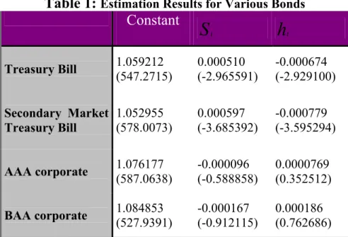
Estimation results for equation (8) are reported in Table 1.

Table 1:

Estimation Results for Various Bonds

Constant

S

h

Treasury Bill

1.059212

_(547.2715)

0.000510

_(-2.965591)

-0.000674

_(-2.929100)

Secondary Market

Treasury Bill

1.052955

(578.0073)

0.000597

(-3.685392)

-0.000779

(-3.595294)

AAA corporate

1.076177

_(587.0638)

-0.000096

_(-0.588858)

0.0000769

_(0.352512)

BAA corporate

1.084853

_(527.9391)

-0.000167

_(-0.912115)

0.000186

_(0.762686)

Note: t-statistics are reported in parentheses.

As it can be seen from Table 1, treasury bills seem to be positively correlated with

structural uncertainty, and negatively correlated with impulse uncertainty. However,

results for corporate bonds are not significant. These results show us that, as the

impulse uncertainty increases, volatility shocks to the economy rise, agents fly to the

treasury bonds, and since the demand to these bonds increase, their prices decrease.

Nevertheless, it is hard to make such an interpretation for corporate bonds due to the

insignificant estimation results

. So by looking the effects of inflation uncertainty on

the interest rates separately, it is difficult to say there is a flight to quality effect, but

we can test this effect by analysing the relationship between uncertainties and

interest rate spreads.

3.3 Testing the “Flight to Quality” Hypothesis

In order to test whether

‘Flight to Quality’ hypothesis holds for spreads, we estimate

the following equation by using least square estimation method:

t

t

t

t

h

S

Spread

=

α

₀

+

α

₁

+

α

₂

+

ε

₍₉₎

The

‘Flight to Quality’ hypothesis suggests that there has to be a positive relationship

between impulse uncertainty and spreads

. As the impulse uncertainty increases, it

means that there are sudden shocks that hit the economy, and this leads investors not

to hold the risky bonds, corporate bonds, and prefer more safer bonds, such as

treasury bills. By this way, the demand for corporate bonds decreases relatively to

the demand for the treasury bills, which in turn causes the change in the value of

corporate bonds to be higher than the change in the value of treasury bills.

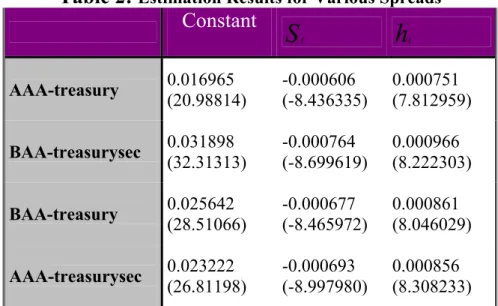
The estimation results for equation (9) are reported in Table 2. Results show us that

impulse uncertainty has a significantly positive effect on the spreads while structural

uncertainty has a significantly negative effect on the spreads, which is in favour of

‘Flight to Quality’ hypothesis. The reason for not having a positive relationship

between structural uncertainty and spreads is that the spreads we analysed in this

paper are all short-term bonds (all have 3 month maturity). Therefore the changes in

14 _{See Fisher (1959) and Litterman and Iben (1991). Fisher (1959) suggests that there is a positive} relationship between default risk and yield spreads, while Litterman and Iben (1991) suggests that risk

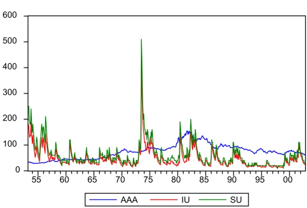
Figure 5

Note: Jointly behaviors of corporate bonds, structural uncertainty and impulse uncertainty

Figure 6

the demand for these bonds will be mostly affected from the sudden shocks that hit

the economy, impulse uncertainty, rather than the uncertainty of the structure of the

economy.

3.4 Robustness of Estimation Results

As indicated above, BAA-treasury, BAA-treasurysec, and AAA-treasurysec spreads

are used for testing the robustness of the results. Using equation (9), these spreads

are regressed on structural uncertainty and impulse uncertainty, generated by using

equations (1) through (7). Results are reported in Table 2. It can be easily seen from

the table that coefficients of structural uncertainty in the estimation for all kinds of

spreads are negative, as it is in the original case. Moreover, t-statistics, reported in

the table show us that these coefficients are significant.

Furthermore, all the coefficients for impulse uncertainty are positive, and they are all

significant. So, these findings clearly state that our results remain robust.

Table 2:

Estimation Results for Various Spreads

Constant

S

h

AAA-treasury

0.016965

_(20.98814)

-0.000606

_(-8.436335)

0.000751

_(7.812959)

BAA-treasurysec

0.031898

_(32.31313)

-0.000764

_(-8.699619)

0.000966

_(8.222303)

BAA-treasury

0.025642

_(28.51066)

-0.000677

_(-8.465972)

0.000861

_(8.046029)

AAA-treasurysec

0.023222

_(26.81198)

-0.000693

_(-8.997980)

0.000856

_(8.308233)

4 Conclusion

There is a great literature devoted to link between inflation uncertainty and interest

rates. However, there are opposing findings about the relationship between inflation

uncertainty and interest rates. Some of the studies find a positive correlation between

these two variables, while some of them find a negative correlation. In this paper, we

analyzed the link between inflation uncertainty and spreads among riskier and safer

bonds within a model of a time-varying parameter model with an ARCH

specification. We divided inflation uncertainty into two parts, structural uncertainty

and impulse uncertainty, as indicated in Evans (1991), firstly. We estimated the

relationship between these types of uncertainties and spreads among riskier and safer

bonds, using USA data.

The results indicate us that both structural and impulse uncertainties have significant

relationship with the spreads between corporate bonds, the riskier bonds, and

treasury bills, the safer bonds. Impulse uncertainty has a positive effect on spreads,

which is an evidence for ‘Flight to Quality’ hypothesis. As the sudden shocks hit the

economy, an indication of a rise in impulse uncertainty, people have more doubts for

the returns of riskier bonds than the returns of safer bonds with short-term maturity,

and this leads a more flight from the riskier bonds, compared to the flight from the

safer bonds. So the spread between the riskier bonds and safer bonds increase, which

supports

‘Flight to Quality’ hypothesis. However, structural uncertainty does not

have a positive effect on spreads. This is because of the short-term maturity of the

bonds. All the interest rate spreads are generated by using 3-months maturity bonds.

We expect a change in the demand of these bonds due to the sudden volatilities in the

economy, rather than the structural modifications. Therefore, it is anticipated not to

have a positive relationship between structural uncertainty and spreads.

BIBLIOGRAPHY

Aghion, P., and P. Bolton (1993), “A Theory of Trickle-Down Growth and

Development with Debt Overhang,” unpublished, Nuffield College (Oxford) and

LSE.

Athanassakos, G., P. Carayannopoulos (2001), “An Empirical Analysis of the

Relationship of Bond Yield Spreads and Macro-economic Factors,” Applied

Financial Economics 11, 197-207.

Ball, L. and S. Cecchetti (1990), “Inflation Uncertainty at Short and Long Horizons,”

Brookings Papers on Economic Activity, 215-254.

Ball, L. (1992), “Why does High Inflation Raise Inflation Uncertainty,”

Journal of

Monetary Economics 1, 371-388.

Ball, L., N. G. Mankiw, and D. Romer (1988), “The New Keynesian Economics and

the Output-Inflation Trade-off,”

Brookings Papers on Economic Activity, no.1, 1-65.

Bernanke, B. and A. Blinder (1988), “Credit, Money and Aggregate Demand,”

American Economic Review 98, 435-439.

Bernanke, B. and M. Gertler (1989), “Agency Costs, Net Worth and Business

Fluctuations,”

American Economic Review 79, 14-31.

Bernanke, B. and M. Gertler (1990), “Financial Fragility and Economic

Performance,”

Quarterly Journal of Economics 105, 87-114.

Berument, H. (1999), “The Impact of Inflation Uncertainty on Interest Rates in the

UK,”

Scottish Journal of Political Economy 46, 207-218.

Berument, Hakan, Zubeyir Kilinc and Umit Ozlale (2002), “The Missing Link

Between Inflation Uncertainty and Interest Rates,” unpublished, Bilkent University

(Ankara, Turkey).

Berument, Hakan, Zubeyir Kilinc and Umit Ozlale (2003), “Long-Short Interest Rate

Spreads and Different Inflation Risk Premiums”, unpublished, Bilkent University

(Ankara, Turkey).

Blanchard, O. J. and S. Fischer (1989), Lectures on Macroeconomics, Cambridge,

Mass.: MIT Press.

Bollersev, T. (1986), “Generalized Autoregressive Conditional Heteroskedasticity, ”

Journal of Econometrics 31, 307-327.

Bomberger, T. (1996), “Disagreement as a Measure of Uncertainty,”

Journal of

Money, Credit, and Banking 23(3), 381-392.

Calomiris, C. and R. G. Hubbard (1990), “Imperfect Information, Multiple Loan

Markets and Credit Rationing,” Economic Journal 100.

Carey, M., S. Browse, J. Rea, and G. Udell (1993), “The Economics of the Private

Placement Market,” preliminary staff study, Board of Governors.

Chan, L. K. C. (1994), “Consumption, Inflation Risk, and Real Interest Rates: An

Empirical Analysis,” Journal of Business 67, 69-96.

Chow, G. C. (1984),

Econometrics, New York: McGraw-Hill.

Corcoran, P. (1992), “The Credit Slowdown of 1989-1991: The Role of Supply and

Demand,” Federal Reserve Bank of Chicago,

Proceedings of the 28

Annual

Conference on Bank Structure and Competition.

Cukierman, A. and P. Wachtel (1979), “Differential inflationary expectations and the

variability of the rate of inflation,”

American Economic Review 69, 595-609.

Cukierman, A. and P. Wachtel (1982), “Relative Price Variability and Nonuniform

Inflationary Expectations,”

Journal of Political Economy 90, 146-157.

Cukierman, A., and A. Meltzer (1986), “A Theory of Ambiguity, Credibility, and

Inflation Under Discretion and Asymmetric Information,”

Econometrica 17,

1099-1128.

Darby, M. R. (1975), “The Financial and Tax Effects of Monetary Policy on Interest

Rates,”

Economic Inquiry 13, 266-276.

Davis, G., and B. Kanago (1996), “On Measuring the Effect of Inflation Uncertainty

on Real GNP,”

Oxford Economic Papers 48, 163-175.

Duffee, G. R. (1996), “Treasury Yields and Corporate Bond Yield Spreads: An

Empirical Analysis,” unpublished, Federal Reserve Board.

Duffee, G. R. (1998), “The Relation Between Treasury Yields and Corporate Bond

Yield Spreads,” Journal of Finance 53, 2225-2240.

Duffie, D. and K. Singleton (1997), “An econometric Model of the Term Structure of

Interest Rate Swap Yields,”

Journal of Finance 52, 1287-1322.

Eichengreen, B., G. Hale, A. Mody (2000), “Flight to Quality: Investor Risk

Tolerance and the Spread of Emerging Market Crises,” working paper, World Bank.

Elton, E., M. J. Gruber, D. Agrawal, C. Mann (2001), “Explaining the Rate Spread

on Corporate Bonds”, The Journal of Finance 56, 247-277.

Evans, M. (1989), “On the Changing Nature of the Output-Inflation Tradeoff”,

Working Paper, Solomon Brothers Research Center, Stern School of Business, New

York University.

Evans, M. (1991), “Discovering the Link Between Inflation Rates and Inflation

Uncertainty,” Journal of Money, Credit, and Banking 23, 169-184.

Evans, M. and P. Wachtel (1993), “Inflation Regimes and the Sources of Inflation

Uncertainty,”

Journal of Money, Credit, and Banking 25, 475-511.

Fama, E. (1975), “Short Term Interest Rates as Predictor of Inflation,”

American

Economic Review 65, 269-282.

Fama, E. and M. Gibbons (1982), “Inflation, Real Returns and Capital Investment,”

Journal of Monetary Economics 9, 297-323.

Fama, E., and K. French (1993), “Common Risk Factors in the Returns on Stocks

and Bonds,”

Journal of Financial Economics 33, 3-57.

Fisher, L. (1959), “Determinants of Risk Premiums on Corporate Bonds”,

Journal of

Political Economy 67, 217-230.

Friedman, M. (1977), “Nobel Lecture: Inflation and Unemployment,”

Journal of

Political Economy 85, 451-472.

Froyen, R. and R. Waud (1987), “An Examination of Aggregate Price Uncertainty in

Four Countries and Some Implications for Real Output,”

International Economic

Review, 353-373.

Gertler, M. (1992), “Financial Capacity and Output Fluctuations in an Economy with

Multiperiod Financial Relationships,”

Review of Economic Studies 59, 455-472.

Gertler, M. and S. Gilchrist (1993), “The Role of Credit Market Imperfections in the

Monetary Transmission Mechanism: Arguments and Evidence,”

Scandinavian

Journal of Economics, 309-340.

Hafer, R. W. (1986), “Inflation Uncertainty and a Test of the Friedman Hypothesis,”

Journal of Macroeconomics, 365-372.

Holland, S. (1986). “Wage Indexation and the Effect of Inflation Uncertainty on Real

GNP,”

Journal of Business, 473-484.

Holland, S. (1988), “Indexation and the Effect of Inflation Uncertainty on

Employment: An Empirical Analysis,”

American Economic Review, 235-244.

Holland, S. (1993b), “Comment on Inflation Regimes and the Sources of Inflation

Uncertainty,”

Journal of Money, Credit, and Banking 27, 514-520.

Holland, S. (1995), “Inflation and Uncertainty: Test for Temporal Ordering,”

Journal

of Money, Credit, and Banking 27, 827-837.

Kashyap, A. and J. Stein (1994), “Monetary Policy and Bank Lending,” in N.

Gregory Mankiw (ed.),

Monetary Policy (Chicago:University of Chicago Press for

Kashyap, A., J. Stein, and D. Wilcox (1993), “Monetary Policy, and Credit

Conditions: Evidence from the Composition of External Finance,” American

Economic Review 83, 78-98.

Lang, W. and L. Nakamura (1992), “‘Flight to Quality’ in Bank Lending and

Economic Activity,” unpublished, Federal Reserve Bank of Philadelphia.

Litterman, R. and T. Iben (1991), “Corporate Bond Valuation and the Term Structure

of Credit Spreads,” The Journal of Portfolio Management, 52-64.

Morgan, D. (1993), “The Lending View of Monetary Policy and Bank Loan

Commitments,” unpublished, Federal Reserve Bank of Kansas City.

Mullineaux, D. J. (1980), “Unemployment, Industrial Production and Inflation

Uncertainty in United States,” Review of Economics and Statistics 2, 1-32.

Oliner, S., and G. Rudebusch (1993), “Is There a Bank Credit Channel to Monetary

Policy,” unpublished, Board of Governors.

Platt, H., and M. Platt (1992), “Credit Risk and Yield Differentials for High Yield

Bonds,” Quarterly Journal of Business and Economics 31, 51-68.

Rodrigues, A. P. (1997), “Term Structure and Volatility Shocks,” unpublished,

Federal Reserve Bank of New York.

Routledge, B. R., S. E. Zin (2001), “Model Uncertainty and Liquidity,” NBER

Working Paper.

Severn, A. K., and W. J. Stewart (1992), “The Corporate-Treasury Yield Spread and

State Taxes,” Journal of Economics and Business 44, 161-166.

Summers, L. H. (2000), “International Financial Crises: Causes, Prevention, and

Cures,”

American Economic Review –Papers and Proceedings 90(2), 1-17.

Townsend, R. (1979), “Optimal Contracts and Competitive Markets with Costly

State Verification,”

Journal of Economic Theory 21, 265-293.

Williamson, S. (1989), “Costly Monitoring, Optimal Contracts and Liquidity

APPENDIX A

(MATLAB CODES FOR THE MODEL)

FUNCTION 1

%--- % USAGE: tvp_garchd

%--- % State-Space Models with Regime Switching load usinf.data; y = usinf(:,1); n = length(y); x = [ones(n,1) usinf(:,2:13)]; % global y; % global x; [n k] = size(x); % initial values parm = [1.924010 0.250715 0.084523 0.099977 0.044039 0.042374 0.067159 0.029956 0.089208 0.096543 0.099444 0.034634 -0.091534 4.773617 0.147682 0.807179 ];

info.b0 = zeros(k+1,1); % relatively diffuse prior info.v0 = eye(k+1)*50;

info.prt = 1; % turn on printing of some %intermediate optimization results info.start = 11; % starting observation result = tvp_garch(y,x,parm,info) vnames =

strvcat('inflation','constant','inflation1','inflation2','inflation3','inflation4','inflation5','inflation6','inflatio n7','inflation8','inflation9','inflation10','inflation11','inflation12')

FUNCTION 2

function result = tvp_garch(y,x,parm,info)

% PURPOSE: time-varying parameter estimation with garch(1,1) errors % y(t) = X(t)*B(t) + e(t), e(t) = N(0,h(t))

% B(t) = B(t-1) + v(t), v(t) = N(0,sigb^2)

% h(t) = a0 + a1*e(t-1)^2 + a2*h(t-1) ARMA(1,1) error variances % ---

% USAGE: result = tvp_garch(y,x,parm,info);

% or: result = tvp_garch(y,x,parm); for default options % where: y = dependent variable vector

% x = explanatory variable matrix % parm = (k+3)x1 vector of starting values % parm(1:k,1) = sigb vector

% parm(k+1,1) = a0 % parm(k+2,1) = a1 % parm(k+3,1) = a2

% info = a structure variable containing optimization options

% info.b0 = a (k+1) x 1 vector with initial b values (default: zeros(k+1,1)) % info.v0 = a (k+1)x(k+1) matrix with prior for sigb

% (default: eye(k+1)*1e+5, a diffuse prior) % info.prt = 1 for printing some intermediate results % = 2 for printing detailed results (default = 0)

% info.delta = Increment in numerical derivs [.000001] % info.hess = Hessian: ['dfp'], 'bfgs', 'gn', 'marq', 'sd'

% info.maxit = Maximium iterations [500]

% info.lamda = Minimum eigenvalue of Hessian for Marquardt [.01] % info.cond = Tolerance level for condition of Hessian [1000] % info.btol = Tolerance for convergence of parm vector [1e-4] % info.ftol = Tolerance for convergence of objective function [sqrt(eps)] % info.gtol = Tolerance for convergence of gradient [sqrt(eps)] % info.start = starting observation (default: 2*k+1)

% --- % RETURNS: a result structure

% result.meth = 'tvp_garch'

% result.sigb = a (kx1) vector of sig beta estimates % result.ahat = a (3x1) vector with a0,a1,a2 estimates

% result.vcov = a (k+3)x(k+3) var-cov matrix for the parameters % result.tstat = a (k+3) x 1 vector of t-stats based on vcov

% result.stdhat = a (k+3) x 1 vector of estimated std deviations % result.beta = a (start:n x k) matrix of time-varying beta hats % result.ferror = a (start:n x 1) vector of forecast errors % result.fvar = a (start:n x 1) vector for conditional variances % result.sigt = a (start:n x 1) vector of arch variances % result.rsqr = R-squared

% result.rbar = R-bar squared % result.yhat = predicted values % result.y = actual values

% result.like = log likelihood (at solution values) % result.iter = # of iterations taken

% result.start = # of starting observation % result.time = time (in seconds) for solution

% --- % NOTES: 1) to generate tvp betas based on max-lik parm vector % [beta ferror] = tvp_garch_filter(parm,y,x,start,b0,v0);

% 2) tvp_garch calls garch_trans(), maxlik(), tvp_garch_like, tvp_garch_filter % ---

% SEE ALSO: prt(), plt(), tvp_garch_like, tvp_garch_filter % ---

infoz.maxit = 500; [n k] = size(x); start = 2*k+1;

priorv0 = eye(k+1)*1e+5; priorb0 = zeros(k+1,1);

if nargin == 4 % we need to reset optimization defaults if ~isstruct(info)

error('tvp_garch: optimization options should be in a structure variable'); end; % parse options fields = fieldnames(info); nf = length(fields); for i=1:nf if strcmp(fields{i},'maxit') infoz.maxit = info.maxit; elseif strcmp(fields{i},'btol') infoz.btol = info.btol; elseif strcmp(fields{i},'ftol') infoz.ftol = info.ftol; elseif strcmp(fields{i},'gtol') infoz.gtol = info.gtol; elseif strcmp(fields{i},'hess') infoz.hess = info.hess; elseif strcmp(fields{i},'cond') infoz.cond = info.cond; elseif strcmp(fields{i},'prt') infoz.prt = info.prt; elseif strcmp(fields{i},'delta') infoz.delta = info.delta; elseif strcmp(fields{i},'lambda') infoz.lambda = info.lambda; elseif strcmp(fields{i},'start') start = info.start; elseif strcmp(fields{i},'v0') priorv0 = info.v0; elseif strcmp(fields{i},'b0') priorb0 = info.b0; end; end; end;

% Do maximum likelihood estimation

oresult = maxlik('tvp_garch_like',parm,infoz,y,x,start,priorb0,priorv0); parm1 = oresult.b;

% take absolute value of standard deviations parm1(1:k,1) = abs(parm1(1:k,1));

niter = oresult.iter; like = -oresult.f; time = oresult.time;

% compute numerical hessian at the solution

cov0 = inv(fdhess('tvp_garch_like',parm1,y,x,start,priorb0,priorv0)); grad = fdjac('garch_trans',parm1);

vcov = grad*cov0*grad'; stdhat = sqrt(diag(vcov));

% produce tvp beta hats,

% prediction errors and variance of forecast error, % and garch(1,1) variance estimates

[beta ferror fvar sigt] = tvp_garch_filter(parm1,y,x,start,priorb0,priorv0);

% transform a0,a1,a2 parm1 = garch_trans(parm1); yhat = zeros(n-start+1,1); for i=start:n; yhat(i-start+1,1) = x(i,:)*beta(i-start+1,:)'; end;

resid = y(start:n,1) - yhat; sigu = resid'*resid; tstat = parm./stdhat; ym = y(start:n,1) - mean(y(start:n,1)); rsqr1 = sigu; rsqr2 = ym'*ym; result.rsqr = 1.0 - rsqr1/rsqr2; % r-squared rsqr1 = rsqr1/(n-start); rsqr2 = rsqr2/(n-1.0); result.rbar = 1 - (rsqr1/rsqr2); % rbar-squared % return results structure information result.sigb = parm1(1:k,1); result.ahat = parm1(k+1:k+3,1); result.beta = beta; result.ferror = ferror; result.fvar = fvar; result.sigt = sigt; result.vcov = vcov; result.yhat = yhat; result.y = y; result.resid = resid; result.like = like; result.time = time; result.tstat = tstat; result.stdhat = stdhat; result.nobs = n; result.nvar = k; result.iter = niter; result.meth = 'tvp_garch'; result.start = start; FUNCTION 3

function result = maxlik(func,b,info,varargin) % PURPOSE: minimize a log likelihood function % --- % USAGE: result = maxlike(func,b,info,varargin)

% or: result = maxlike(func,b,[],varargin) for default options % Where: func = function to be minimized

% info structure containing optimization options

% .delta = Increment in numerical derivs [.000001] % .hess = Hessian method: ['dfp'], 'bfgs', 'gn', 'marq', 'sd' % .maxit = Maximium iterations [100]

% .lambda = Minimum eigenvalue of Hessian for Marquardt [.01] % .cond = Tolerance level for condition of Hessian [1000] % .btol = Tolerance for convergence of parm vector [1e-4] % .ftol = Tolerance for convergence of objective function [sqrt(eps)] % .gtol = Tolerance for convergence of gradient [sqrt(eps)] % .prt = Printing: 0 = None, 1 = Most, 2 = All [0]

% varargin = arguments list passed to func

% --- % RETURNS: results = a structure variable with fields: % .b = parameter value at the optimum % .hess = numerical hessian at the optimum % .bhist = history of b at each iteration

% .f = objective function value at the optimum % .g = gradient at the optimum

% .dg = change in gradient % .db = change in b parameters % .df = change in objective function % .iter = # of iterations taken

% .meth = 'dfp', 'bfgs', 'gn', 'marq', 'sd' (from input) % .time = time (in seconds) needed to find solution % --- infoz.func = func; % set defaults infoz.maxit = 100; infoz.hess = 'bfgs'; infoz.prt = 0; infoz.cond = 1000; infoz.btol = 1e-4; infoz.gtol = sqrt(eps); infoz.ftol = sqrt(eps); infoz.lambda = 0.01; infoz.H1 = 1; infoz.delta = .000001; infoz.call = 'other'; infoz.step = 'stepz'; infoz.grad='numz'; hessfile = 'hessz'; if length(info) > 0 if ~isstruct(info)

error('maxlik: options should be in a structure variable'); end;

% parse options

fields = fieldnames(info);

nf = length(fields); xcheck = 0; ycheck = 0; for i=1:nf if strcmp(fields{i},'maxit') infoz.maxit = info.maxit; elseif strcmp(fields{i},'btol') infoz.btol = info.btol; elseif strcmp(fields{i},'gtol')

infoz.gtol = info.gtol; elseif strcmp(fields{i},'ftol') infoz.ftol = info.ftol; elseif strcmp(fields{i},'hess') infoz.hess = info.hess; elseif strcmp(fields{i},'cond') infoz.cond = info.cond; elseif strcmp(fields{i},'lambda') infoz.lambda = info.lambda; elseif strcmp(fields{i},'delta') infoz.delta = info.delta; elseif strcmp(fields{i},'prt') infoz.prt = info.prt; end; end; else

% rely on default options end; lvar = length(varargin); stat.iter = 0; k = rows(b); if lvar > 0 n = rows(varargin{1}); end; convcrit = ones(4,1); stat.Hi = []; stat.df = 1000; stat.db = ones(k,1)*1000; stat.dG = stat.db; func = fcnchk(infoz.func,lvar+2); grad = fcnchk(infoz.grad,lvar+1); hess = fcnchk(hessfile,lvar+2); step = fcnchk(infoz.step,lvar+2); stat.f = feval(func,b,varargin{:}); stat.G = feval(grad,b,infoz,stat,varargin{:}); stat.star = ' '; stat.Hcond = 0; %==================================================================== % MINIMIZATION LOOP %==================================================================== if infoz.prt > 0

% set up row-column formatting for mprint of intermediate results in0.fmt = strvcat('%5d','%16.8f','%16.8f');

% this is for infoz.prt = 1 (brief information)

in1.cnames = strvcat('iteration','function value','dfunc'); in1.fmt = strvcat('%5d','%16.8f','%16.8f');

% this is for infoz.prt = 2 Vname = 'Parameter'; for i=1:k tmp = ['Parameter ',num2str(i)]; Vname = strvcat(Vname,tmp); end; in2.cnames = strvcat('Estimates','dEstimates','Gradient','dGradient'); in2.rnames = Vname; in2.fmt = strvcat('%16.8f','%16.8f','%16.8f','%16.8f');

end

if infoz.prt == 1

mprint([stat.iter stat.f stat.df],in1); end;

if infoz.prt == 2

mprint([stat.iter stat.f stat.df],in1); mprint([b stat.db stat.G stat.dG],in2); end;

t0 = clock;

while all(convcrit > 0)

% Calculate grad, hess, direc, step to get new b stat.iter = stat.iter + 1; stat = feval(hess,b,infoz,stat,varargin{:}); stat.direc = -stat.Hi*stat.G; alpha = feval(step,b,infoz,stat,varargin{:}); stat.db = alpha*stat.direc; b = b + stat.db;

% Re-evaluate function, display current status f0 = stat.f; G0 = stat.G; if strcmp(infoz.call,'other'), stat.f = feval(func,b,varargin{:}); stat.G = feval(grad,b,infoz,stat,varargin{:}); else stat.f = feval(func,b,infoz,stat,varargin{:}); stat.G = feval(grad,b,infoz,stat,varargin{:}); end;

% Determine changes in func, grad, and parms if stat.f == 0 stat.df = 0; else stat.df = f0/stat.f - 1; end stat.dG = stat.G-G0; dbcrit = any(abs(stat.db)>infoz.btol*ones(k,1)); dgcrit = any(abs(stat.dG)>infoz.gtol*ones(k,1)); convcrit = [(infoz.maxit-stat.iter); (stat.df-infoz.ftol);... dbcrit; dgcrit];

if stat.df < 0, error('Objective Function Increased'); end X(stat.iter,:) = b';

% print intermediate results if infoz.prt == 1

mprint([stat.iter stat.f stat.df],in1); end;

if infoz.prt == 2

mprint([stat.iter stat.f stat.df],in1); mprint([b stat.db stat.G stat.dG],in2); end;

end

time = etime(clock,t0);

%==================================================================== % FINISHING STUFF

%==================================================================== % Write a message about why we stopped

if infoz.prt > 0 if convcrit(1) <= 0

critmsg = 'Maximum Iterations'; elseif convcrit(2) <= 0

critmsg = 'Change in Objective Function'; elseif convcrit(3) <= 0

critmsg = 'Change in Parameter Vector'; elseif convcrit(4) <= 0

critmsg = 'Change in Gradient'; end

disp([' CONVERGENCE CRITERIA MET: ' critmsg]) disp(' ')

end

% put together results structure information result.bhist = X; result.time = time; result.b = b; result.g = stat.G; result.dg = stat.dG; result.f = stat.f; result.df = stat.df; result.iter = stat.iter; result.meth = infoz.hess;

% Calculate numerical hessian at the solution result.hess = fdhess(func,b,varargin{:});

FUNCTION 4

function llik = tvp_garch_like(parm,y,x,start,priorb0,priorv0) % PURPOSE: log likelihood for tvp_garch model

% ---

% USAGE: llike = tvp_garch_like(parm,y,x,start,priorb0,priorv0) % where: parm = a vector of parmaeters

% parm(1) = sig beta 1 % parm(2) = sig beta 2 % .

% . % .

% parm(k) = sig beta k % parm(k+1) = a0 % parm(k+2) = a1 % parm(k+3) = a2

% start = # of observation to start at % (default: 2*k+1)

% priorb0 = a (k+1)x1 vector with prior for b0 % (default: zeros(k+1,1), a diffuse prior) % priorv0 = a (k+1)x(k+1) matrix with prior for sigb % (default: eye(k+1)*1e+5, a diffuse prior) % ---

% RETURNS: -log likelihood function value (a scalar) % ---

[n k] = size(x);

% transform parameters parm = garch_trans(parm); if nargin == 3

start = 2*k+1; % use initial observations for startup priorv0 = eye(k+1)*1e+5; priorb0 = zeros(k+1,1); elseif nargin == 4 priorv0 = eye(k+1)*1e+5; priorb0 = zeros(k+1,1); elseif nargin == 6 % do nothing else

error('tvp_garch_like: Wrong # of input arguments'); end; sigb = zeros(k,1); for i=1:k; sigb(i,1) = parm(i,1)*parm(i,1); end; a0 = parm(k+1,1); a1 = parm(k+2,1); a2 = parm(k+3,1);

ivar = a0/(1-a1-a2); % initial variance f = eye(k+1);

f(k+1,k+1) = 0; g = eye(k+1); cll = priorb0;

pll = priorv0; % initial var-cov for reg coef pll(k+1,k+1) = ivar; htl = ivar; loglik = zeros(n,1); for iter = 1:n; h = [x(iter,:) 1]; ht = a0 + a1*(cll(k+1,1)*cll(k+1,1) + pll(k+1,k+1)) + a2*htl; tmp = [sigb ht]; Q = diag(tmp); ctl = f*cll; ptl = f*pll*f' + g*Q*g';

vt = y(iter,1) - h*ctl; % prediction error su = h*ptl*h';

ft = h*ptl*h'+ht; % variance of forecast error ctt = ctl + ptl*h'*(1/ft)*vt;