(2017) 25: 1436 – 1447 c ⃝ T¨UB˙ITAK doi:10.3906/elk-1603-33 h t t p : / / j o u r n a l s . t u b i t a k . g o v . t r / e l e k t r i k / Research Article
Truncation thresholds: a pair of spike detection thresholds computed using
truncated probability distributions
Murat OKATAN1,∗, Mehmet KOCAT ¨URK2
1Department of Biomedical Engineering, Faculty of Technology, Cumhuriyet University, Sivas, Turkey 2
Department of Biomedical Engineering, Faculty of Engineering and Natural Sciences, ˙Istanbul Medipol University, ˙Istanbul, Turkey
Received: 04.03.2016 • Accepted/Published Online: 12.05.2016 • Final Version: 10.04.2017
Abstract: We describe a method for computing a pair of spike detection thresholds, called ‘truncation thresholds’,
using truncated probability distributions, for extracellular recordings. In existing methods the threshold is usually set to a multiple of an estimate of the standard deviation of the noise in the recording, with the multiplication factor being chosen between 3 and 5 according to the researcher’s preferences. Our method has the following advantages over these methods. First, because the standard deviation is usually estimated from the entire recording, which includes the spikes, it increases with firing rate. By contrast, truncation thresholds decrease in absolute value with increasing firing rate, thereby capturing more of the signal. Second, the parameters of the selected noise distribution are estimated more accurately by maximum likelihood fitting of the truncated distribution to the data delimited by the truncation thresholds. Third, the computation of the truncation thresholds is completely data-driven. It does not involve a user-defined multiplication factor. Fourth, methods that use a threshold that is proportional to the estimated standard deviation of the noise assume that the noise distribution is symmetrical around the mean. By contrast, truncation thresholds are not linked to each other by an assumption of symmetry about some axis. Fifth, existing methods do not verify that subthreshold data obey a noise distribution. Truncation thresholds, however, are defined by the fact that the distribution of the data they delimit is statistically indistinguishable, according to the Kolmogorov–Smirnov test, from a selected distribution, truncated at those thresholds. Application of the method is illustrated using recordings from cortical area M1 in awake behaving rats, as well as in simulated recordings. Source code and executables of a software suite that computes the truncation thresholds are provided for the case when the noise distribution is modeled as truncated normal.
Key words: Biomedical signal processing, brain–machine interfaces, microelectrode recordings, computational
neuro-science
1. Introduction
Extracellular recordings of neuronal activity provide information about the electrical activity of both individual and populations of neurons [1,2]. Extracellular recordings are widely used in behavioral neuroscience in exploring the information processing that takes place at the level of individual and populations of neurons [3]. In humans, such recordings are usually performed in the clinical setting, as in perioperative investigations in epilepsy [4] or in the use of brain–machine interfaces in patients with spinal cord injuries [5].
In most studies, the detection of action potentials, or spikes, constitutes one of the first steps in the use of ∗Correspondence: [email protected]
extracellular neural recordings [6]. Because spikes stand out in these data as relatively large amplitude events, the easiest and most straightforward method for detecting them is amplitude thresholding. The threshold is usually set to k× ˆσ , where ˆσ is an estimate of the standard deviation of the noise in the recording and k is a multiplication factor that is usually chosen to be between 3 and 5 depending on the researcher’s preferences [7–11]. However, this method of determining the threshold has some drawbacks. First, the use of such a multiplication factor ( k) adds an element of subjectivity to spike detection. In addition, the standard deviation estimate ( ˆσ) increases with the spiking frequency of the recorded neurons [7]. This is undesired since an increase
in spiking frequency, or firing rate, does not necessarily imply an increase in the standard deviation of the noise that is present in the recording. As a consequence of the firing rate-dependent increase in both ˆσ and the
threshold that is proportional to ˆσ , more action potentials may be missed at high firing rates. Apart from the
dependence on firing rate, choosing k high is likely to result in some action potentials being classified as noise, whereas choosing it low is likely to result in some noise events being classified as spike candidates. Evidence suggests that suprathreshold events carry information regardless of whether they can be identified as individual spikes [11]. These findings and observations underline the importance of using an objective and accurate method for computing spike detection thresholds that can efficiently separate signal and noise. Accordingly, this study addresses the question of whether spikes in extracellular recordings can be detected through thresholding in a principled way that is completely independent of the researcher. To address this issue, a method of computing a pair of spike detection thresholds, called ‘truncation thresholds’, is developed, and its application is illustrated in extracellular recordings obtained from cortical area M1 in awake behaving rats, as well as in simulated spike trains. The method has general applicability to problems where a continuous-valued data set needs to be segmented into two nonoverlapping parts such that one part obeys a desired continuous-valued truncated distribution while the other does not. Preliminary results of this study have been published in [12,13].
2. Materials and methods
This section explains the computation of the truncation thresholds along with the real and simulated neural data that are used for illustrating their application. All computations were performed in MATLAB (R2015a, MathWorks, Inc., USA) under a 64 bit Windows 8.1 Single Language (2013) operating system on a laptop computer with 6 GB RAM and 2.60 GHz Intel⃝CoreR TMi5-3230M CPU.
2.1. Mathematical representation of the recordings
Because extracellular neural recordings are typically acquired using analog to digital conversion systems, their initial representation in digital form is a discrete-time discrete-valued time series. Let d [n] , 0≤ n ≤ N − 1, denote such a recording, with N representing the total number of samples in the recording. The method presented here computes the spike detection thresholds by verifying that the samples that lie between the thresholds obey a truncated continuous-valued probability distribution function. This verification is performed using the Kolmogorov–Smirnov (KS) test. Because d [n] is discrete-valued, the distribution of its samples will likely deviate significantly from a continuous distribution for any reasonable choice of thresholds, which implies that the method proposed here may not be applied directly on d [n] . Fortunately, spike detection is usually not performed directly on d [n] , but rather on a band-pass filtered version of it, in which frequencies below a few hundred Hz and above a few kHz are attenuated. This filtering is expected to convert d [n] into a time series that can be considered continuous-valued for the purposes of the present method. Let x [n] denote this filtered recording. The following analysis assumes that the spikes will be detected in x [n] and that x [n] is a continuous-valued discrete-time signal.
2.2. Basic premises of truncation thresholds
Extracellular recordings are often assumed to consist of background activity and action potentials, or spikes. The background activity is assumed to arise from the superimposed electrical activities of large numbers of neurons that are located at various distances relative to the recording electrode and that are usually asynchronous. Therefore, background activity is usually considered noise [7,14,15]. Consistent with this characterization, the present analysis assumes that there exist threshold pairs Θ = [θl,θh] , min (x)≤ θl< θh≤ max (x), such that
the samples that are between these thresholds, zΘ ∈ {x [n] | θl≤ x [n] ≤ θh}, obey a parametric
continuous-valued noise distribution F (
z| ˆζΘ
)
that is truncated at θl and θh, where ˆζΘ is the parameter vector that is
estimated from zΘ by maximum likelihood. Note that each selection of Θ defines a zΘ and a ˆζΘ. It is accepted
that the truncated distribution F (
z| ˆζΘ
)
fits the truncated data if the KS test yields a P-value that is at least
α . Clearly, for any choice of Θ , a KS P-value is obtained. Let PKS(Θ) denote this value. The largest amount
of noise, under F (
z| ˆζΘ
)
, is segmented out of x , by the value of Θ that maximizes ∆ (Θ)≜ θh−θl and for
which PKS(Θ)≥ α. Let this optimal solution be denoted by ˆΘo. Since x is assumed to be continuous-valued,
it may contain about N distinct values, each of which is a candidate for θl or θh. Thus, it may be presumed
that there are about N (N− 1) /2 different choices of Θ that need to be evaluated in order to find ˆΘo. For
any recording of practical use, this number is prohibitively large. Therefore, rather than aiming at the optimal solution by evaluating all possible values of Θ , a method needs to be adopted that yields a solution with large ∆ (Θ) and that can be computed relatively faster. The method presented here computes such a solution, and the resulting thresholds, denoted by ˆΘt, are called ‘truncation thresholds’.
The computation of ˆΘt involves two steps. In the first step, initial values for the lower and upper
thresholds are computed using the bisection method [16] under the constraint that the other threshold is fixed at the median of x . That is, ˆΘl|m≜
[ ˆ θl|m, median (x) ] and ˆΘh|m≜ [ median (x) , ˆθh|m ]
values are computed as explained in Section 2.3. In the second step the interval
[ ˆ
θl|m, ˆθh|m
]
is stretched or compressed, anchored at the median, using the bisection method, to yield ˆΘt, as explained in Section 2.4. The median is used as an
anchor because it is expected to be located near the middle of the background activity given that the greater part of x is due to the background activity. Because an ordered threshold pair can also be viewed as an interval, it will be referred to as one when appropriate.
2.3. Computing initial values for the lower and upper thresholds
The lower threshold in ˆΘl|m, ˆθl|m, is searched using the bisection method in a set of candidate solutions
that is reduced down to half of its size after each bisection. The initial value of this set is defined as
SCSl|m[1] = {x [n] | x [n] < median (x)}. The solution is obtained after at most I iterations, where I is
the smallest integer that is greater than or equal to log2(K) and K is the cardinality of SCSl|m[1] .
The solution candidate at iteration i is defined as θl|m[i] , which is the sample that is closest to median(SCSl|m[i]
)
. This yields the threshold pair Θl|m[i] =
[ θl|m[i] , median (x) ] . If PKS ( Θl|m[i] ) ≥ α,
then the data that lie in the interval Θl|m[i] are accepted to obey the truncated noise distribution F
(
z| ˆζA[i]
) , where A[i] = Θl|m[i] . This implies that the search for the solution can continue in the set SCSl|m[i + 1] =
{ x [n]∈ SCSl|m[i]| x [n] < θl|m[i] } . If, however, PKS ( Θl|m[i] )
< α , then the data that lie in the interval
Θl|m[i] are not accepted to obey F
(
z| ˆζA[i]
)
. This implies that the search for the solution can continue in the set SCSl|m[i + 1] =
{
x [n]∈ SCSl|m[i]| x [n] > θl|m[i]
}
. This iterative search continues until the cardinality of the set of candidate solutions becomes zero. After the iteration terminates, a search is conducted over all solution candidates Θl|m[i] , 1≤ i ≤ I , to find the one that maximizes ∆
( Θl|m[i]
)
and for which PKS
( Θl|m[i]
)
≥ α.
Let ˆΘl|m denote this solution.
The upper threshold in ˆΘh|m, ˆθh|m, is searched in a similar manner. This time the initial value of the
set of candidate solutions is defined as SCSh|m[1] ={x [n] | x [n] > median (x)}. The solution is obtained after
at most J iterations, where J is the smallest integer that is greater than or equal to log2(L) and L is the cardinality of SCSh|m[1] . The solution candidate at iteration i is defined as θh|m[i] , which is the sample
that is closest to median(SCSh|m[i]
)
. This yields the threshold pair Θh|m[i] =
[ median (x) , θh|m[i] ] . If PKS ( Θh|m[i] )
≥ α, then the data that lie in the interval Θh|m[i] are accepted to obey the truncated noise
distribution F (
z| ˆζB[i]
)
, where B[i] = Θh|m[i] . This implies that the search for the solution can continue in
the set SCSh|m[i + 1] = { x [n]∈ SCSh|m[i]| x [n] > θh|m[i] } . If, however, PKS ( Θh|m[i] )
< α , then the data
that lie in the interval Θh|m[i] are not accepted to obey F
(
z| ˆζB[i]
)
. This implies that the search for the solution can continue in the set SCSh|m[i + 1] =
{
x [n]∈ SCSh|m[i]| x [n] < θh|m[i]
}
. This iterative search continues until the cardinality of the set of candidate solutions becomes zero. After the iteration terminates, a search is conducted over all solution candidates Θh|m[i] , 1≤ i ≤ J , to find the one that maximizes ∆
( Θh|m[i]
) and for which PKS
( Θh|m[i]
)
≥ α. Let ˆΘh|m denote this solution.
If both PKS ( Θl|m[i] ) < α for 1≤ i ≤ I and PKS ( Θh|m[i] )
< α for 1≤ i ≤ J , then neither ˆΘl|m nor
ˆ
Θh|m could be found, which implies that ˆΘt could not be found either. If only ˆΘl|m or ˆΘh|m is found, then
the one that is found equals ˆΘt. If both ˆΘl|m and ˆΘh|m are found, then ˆΘt is computed as explained next.
2.4. Computing the truncation thresholds from the initial values
The threshold pairs ˆΘl|m and ˆΘh|m represent two intervals, below and above median (x) respectively, in which
the data obey the respective truncated distributions with PKS
( ˆ Θl|m ) ≥ α and PKS ( ˆ Θh|m ) ≥ α. The goal
of the present analysis is to find a single pair of thresholds ˆΘt ≜
[ ˆ
θt1, ˆθt2
]
, that will be a wide interval in which the data obey the respective truncated distribution with PKS
( ˆ Θt
)
≥ α. This interval is constructed by
merging the intervals ˆΘl|m and ˆΘh|m and then scaling the resulting interval, anchored at the median, by the
bisection method, as explained next. First, the threshold pair ˆΘw ≜
[ ˆ
θl|m, ˆθh|m
]
is obtained by using the lower and upper thresholds in ˆ
Θl|m and ˆΘh|m respectively, and its adequacy is assessed. The search for the truncation thresholds proceeds
differently depending on whether PKS
( ˆ Θw
)
2.4.1. Computation of the truncation thresholds when PKS ( ˆ Θw ) ≥ α If PKS ( ˆ Θw )
≥ α, then it is inferred that the interval ˆΘw can be widened, unless it already is the widest possible
interval. ˆΘw is the widest possible interval if ˆΘw= [min (x) , max (x)] . In that case the truncation thresholds
are found as ˆΘt = ˆΘw = ˆΘo. If ˆΘw is not the widest possible interval, however, then it is inferred that the
truncation thresholds may correspond to an interval that is wider than ˆΘw. In that case ˆΘt is computed
as Θt
( ˆ
ϕ
)
using Eq. (1), where ˆϕ is a factor that is determined from the data by the bisection method, as
explained next.
Θt(ϕ) = (1− ϕ) × median (x) + ϕ × ˆΘw (1)
Since the role of Θt(ϕ) is to partition the samples in x into two classes, one noise and the other nonnoise,
it suffices if the upper or the lower threshold in Θt(ϕ) , or both, are in {x [n] | x [n] ̸= median (x)}. Let Sl+,
defined in Eq. (2), denote the set of factors that adjust the lower threshold to any of the samples in x that are smaller than ˆθl|m: Sl+= { median (x)− x [n] median (x)− ˆθl|m | x [n] < ˆθl|m } (2)
Let Sh+, defined in Eq. (3), denote the set of factors that adjust the upper threshold to any of the samples in x that are greater than ˆθh|m:
Sh+= { x [n]− median (x) ˆ θh|m− median (x) | x [n] > ˆθh|m } (3)
Then the set of candidate solutions for ϕ is defined in Eq. (4) at the first iteration of the bisection method:
SCSm+[1] = Sl+∪ Sh+ (4)
The solution for ϕ is obtained after at most M iterations, where M is the smallest integer that is greater than or equal to log2(Q) and Q is the cardinality of SCSm+[1] .
The solution candidate at iteration i is defined as ϕ [i] , which is the element of SCSm+[i] that is
closest to median (SCSm+[i]) . This yields the threshold pair Θt(ϕ [i]) . If PKS(Θt(ϕ [i])) ≥ α, then the
data that lie in the interval Θt(ϕ [i]) are accepted to obey the truncated noise distribution F
(
z| ˆζC[i]
) , where
C[i] = Θt(ϕ [i]) . This implies that the search for the solution can continue in the set SCSm+[i + 1] = {ϕ ∈ SCSm+[i]| ϕ > ϕ [i]}. If, however, PKS(Θt(ϕ [i])) < α , then the data that lie in the interval Θt(ϕ [i])
are not accepted to obey F (
z| ˆζC[i]
)
. This implies that the search for the solution can continue in the set
SCSm+[i + 1] = {ϕ ∈ SCSm+[i]| ϕ < ϕ [i]}. This iterative search continues until the cardinality of the set
of candidate solutions becomes zero. After the iteration terminates, a search is conducted over all solution candidates ϕ [i] , 1≤ i ≤ M , to find the one that maximizes ∆ (Θt(ϕ [i])) and for which PKS(Θt(ϕ [i]))≥ α.
Let ˆϕ denote this solution. If PKS(Θt(ϕ [i])) < α for 1 ≤ i ≤ M , then it is inferred that ˆϕ = 1, since PKS ( ˆ Θw ) ≥ α. Let ˆΘt= Θt ( ˆ ϕ )
2.4.2. Computation of the truncation thresholds when PKS ( ˆ Θw ) < α If PKS ( ˆ Θw )
< α , then it is inferred that the truncation thresholds may correspond to an interval that is
narrower than ˆΘw. In that case ˆΘt is computed as Θt
( ˆ
ϕ
)
using Eq. (1) with a set of candidate solutions that is constructed as follows. Let Sl−, defined in Eq. (5), denote the set of factors that adjust the lower threshold
to any of the samples in x that are greater than ˆθl|m and smaller than the median:
Sl−= { median (x)− x [n] median (x)− ˆθl|m | ˆθl|m< x [n] < median (x) } (5)
Let Sh−, defined in Eq. (6), denote the set of factors that adjust the upper threshold to any of the samples in x that are smaller than ˆθh|m and greater than the median:
Sh−= { x [n]− median (x) ˆ θh|m− median (x) | median (x) < x [n] < ˆθh|m } (6)
Then the set of candidate solutions for ϕ is defined in Eq. (7) at the first iteration of the bisection method:
SCSm−[1] = Sl−∪ Sh− (7)
The solution for ϕ is obtained after at most R iterations, where R is the smallest integer that is greater than or equal to log2(U ) and U is the cardinality of SCSm−[1] .
The solution candidate at iteration i is defined as ϕ [i] , which is the element of SCSm−[i] that is closest
to median (SCSm−[i]) . This yields the threshold pair Θt(ϕ [i]) . If PKS(Θt(ϕ [i]))≥ α, then the search for the
solution can continue in the set SCSm−[i + 1] ={ϕ ∈ SCSm−[i]| ϕ > ϕ [i]}. If, however, PKS(Θt(ϕ [i])) < α ,
then the search for the solution can continue in the set SCSm−[i + 1] = {ϕ ∈ SCSm−[i]| ϕ < ϕ [i]}. This
iterative search continues until the cardinality of the set of candidate solutions becomes zero. After the iteration terminates, a search is conducted over all solution candidates ϕ [i] , 1≤ i ≤ R, to find the one that maximizes ∆ (Θt(ϕ [i])) and for which PKS(Θt(ϕ [i]))≥ α. Let ˆϕ denote this solution. Then the truncation thresholds
are obtained again as ˆΘt= Θt
( ˆ
ϕ
)
. If PKS(Θt(ϕ [i])) < α for 1≤ i ≤ R, then it is inferred that truncation
thresholds could not be found for x .
A software suite that computes the truncation thresholds by modeling the noise using the truncated normal distribution is available at scicrunch.org under RRID:SCR 014637
2.5. Application on real data
Computation of the truncation thresholds is illustrated using data that were recorded in a previous study. The recording was made using a neuroprosthesis design environment [17] from the primary motor cortex (area M1) of a rat during lever-pressing in response to visual stimuli. The data segment that is used here is about 12.6 s long and was recorded with a sampling rate of 40 kHz. It was then digitally band-pass filtered between 400 Hz and 8 kHz using a 4th order Butterworth filter.
A truncated normal probability distribution function (Eq. (8)) is used as the noise model F ( z| ˆζΘˆt ) , where ˆζΘˆt = [ ˆ µΘˆt, ˆσΘˆt ]
is the maximum likelihood estimate of the parameter vector consisting of the mean and the standard deviation. Here Φ (·) is the cumulative standard normal distribution function.
F ( z| ˆζΘˆt ) = ( Φ ( z− ˆµΘˆt ˆ σΘˆt ) − Φ ( ˆ θt1− ˆµΘˆt ˆ σΘˆt )) ( Φ ( ˆ θt2− ˆµΘˆt ˆ σΘˆt ) − Φ ( ˆ θt1− ˆµΘˆt ˆ σΘˆt ))−1 (8)
2.6. Application on simulated data
Simulated neural data were generated and analyzed to determine the dependence of truncation thresholds on firing rate. These analyses also revealed the accuracy with which ˆσΘˆt estimates the noise standard deviation.
Eq. (9) defines the simulated data, which were generated for firing rates f between 0 Hz and 50 Hz with steps of 5 Hz.
yf[n] = g [n] + af[n] (9)
Each yf had a duration of 10 s and was sampled at 40 kHz. The noise was generated as the Gaussian process
defined in Eq. (10)
g [n]∼ N (0, σ) (10)
Here, σ = ˆσΘˆt is the noise standard deviation estimated from the real data, as explained in Sections 2.2–2.5.
The spiking processes af were generated by repeating a single well-isolated spike, obtained from the
real data, according to Poisson processes with specified frequencies. Truncation thresholds computed for yf
are denoted by ˆΘt,f. These thresholds and thresholds proportional to estimated noise standard deviations are
plotted as a function of f to illustrate their dependence on firing rate. A proportionality constant of k = 4 was used as a typical value (e.g., [7]). The two standard deviation estimators that are used in addition to ˆσΘˆt,f are
given in Eq. (11) [18] and Eq. (12), where ˆµf is the mean value of yf.
ˆ σm,f = median (|yf|) ( Φ−1(0.75))−1 (11) ˆ σf = v u u t 1 N N∑−1 n=0 (yf[n]− ˆµf) 2 (12) 3. Results
Truncation thresholds are first computed for real extracellular neural activity data to show that they can be computed under the truncated normal distribution noise model. Next, the results on the firing rate dependence of truncation thresholds and alternative thresholds are illustrated using simulated data.
3.1. Truncation thresholds computed for real data
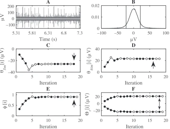
Figure 1 shows a portion of the real data that are used in this study. The duration of this interval is about 2 s and it is located near the middle of the whole recording. Spikes of various amplitudes are visible over a steady background activity. The two horizontal lines show the truncation thresholds that are computed for the whole
recording with α = 0.05 . The location of the truncation thresholds on the 1000 point normalized histogram of the data is also shown. Only the range between ±100 µV is shown for clarity. The number of samples in this recording was N = 504, 735 . Consequently, it took 18 iterations to compute each of ˆθl|m and ˆθh|m, given that log2(N/2) = 17.9 . The values of θl|m[i] and θh|m[i] are shown in Figure 1 for 1 ≤ i ≤ 18. ˆθl|m and ˆθh|m
were found as θl|m[18] =−25.9 µV and θh|m[16] = 23.2 µV , respectively. Upon evaluating PKS
( ˆ Θw
) , it was found to be smaller than α , indicating that ˆϕ needed to be searched in the set of candidate solutions defined
in Eq. (7). The cardinality of this set was U = 438, 034 . Thus, it took 19 iterations to find ˆϕ , given that log2(U ) = 18.7 . ϕ [i] and Θt[i] values are shown in Figure 1 for 1≤ i ≤ 19. ˆϕ was found as ϕ [18] = 0.90.
This resulted in ˆΘt= [−23.4, 20.9] µV .
Time (s)
5.31 5.81 6.31 6.8 7.3μ
V
–100 0 100 200A
µV
–100 –50 0 50 100 0 0.01 0.02B
Iteration
0 5 10 15 20θ
l| m[i
] (
µ
V
)
–40 –20 0C
Iteration
0 5 10 15 20θ
h| m[i] (
µ
V)
0 20 40D
Iteration
Iteration
0 5 10 15 20φ
[i
]
0 0.5 1E
0 5 10 15 20Θ
t[i] (
µ
V
)
–20 0 20F
Figure 1. Computation of the truncation thresholds. (A) A segment of the real extracellular recording after filtering.
Horizontal lines indicate the truncation thresholds. (B) Normalized 1000 point histogram of the samples that make up the filtered recording, shown in the interval ±100 µV. Vertical lines indicate the truncation thresholds. (C–F) The values of θl|m[i] , θh|m[i] , ϕ [i] , and Θt[i] , respectively. Filled circles show solutions for which the KS test P-value is at least 0.05. Arrows indicate ˆθl|m, ˆθh|m, ˆϕ , and ˆΘt.
3.2. Truncation thresholds computed for simulated data
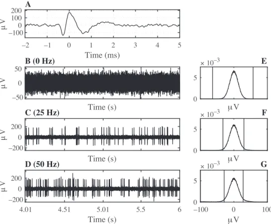
Figure 2 shows the real action potential that was used in generating the simulated data. Segments of simulated data for firing rates of f = 0 Hz, 25 Hz, and 50 Hz are also shown in the figure along with the corresponding truncation thresholds superimposed on 1000 point normalized histograms. Truncation thresholds converged to the minimum and the maximum sample in the recording when f = 0 Hz.
Time (ms)
–2 –1 0 1 2 3 4 5µ
V
–100 0 100 200A
Time (s)
µ
V
–50 0 50B (0 Hz)
μV
× 10–3 0 5E
Time (s)
µ
V
–200 0 200C (25 Hz)
μV
× 10–3 0 5F
Time (s)
4.01 4.51 5.01 5.5 6µ
V
–200 0 200D (50 Hz)
μV
–100 0 100 × 10–3 0 5G
Figure 2. Generation and analysis of simulated data. (A) The well-isolated action potential that was used for generating
the simulated spike trains. (B–D) The sum of simulated noise and spike trains at firing rates of 0 Hz, 25 Hz, and 50 Hz, respectively. Graphs show the central 2 s of 10 s long simulated data. (E–G) Normalized 1000 point histograms of the samples that make up the simulated data. Vertical lines indicate the truncation thresholds.
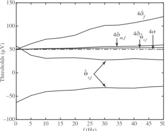
Figure 3 shows ˆΘt,f, the truncation thresholds computed for the simulated data. For comparison 4× ˆσf,
4× ˆσm,f, 4× ˆσΘˆt,f, and 4× σ curves are also plotted. It can be seen that 4 × ˆσf and 4× ˆσm,f increase with
increasing firing rate as expected [7]. Although 4× ˆσΘˆt,f also increases with firing rate, it increases slower than
the latter two. All these thresholds start very close to 4× σ at f = 0 Hz. Unlike these thresholds, truncation thresholds exceed ±4 × σ at f = 0 Hz and decrease in absolute value with increasing firing rate.
4. Discussion
The most widely used method for computing spike detection thresholds is amplitude thresholding using thresh-olds that are proportional to estimated standard deviation of noise. Truncation threshthresh-olds overcome all of the known shortcomings of this method. The results show that truncation thresholds can be computed for real extracellular recordings by modeling the noise using the truncated normal probability distribution (Figure 1). The theory presented here allows computing these thresholds using other continuous-valued probability distributions as the noise model. Alternative models may be explored in future studies.
Analysis results of the simulated data (Figures 2 and 3) showed that the noise standard deviation estimator ˆσΘˆt,f, which is computed as a byproduct of the computation of the truncation thresholds, is more
f (Hz) 0 5 10 15 20 25 30 35 40 45 50 T hre shol ds ( µ V ) –100 –50 0 50 100 150 Θ t,f ^ 4σ 4σ m,f ^ 4σ Θ t,f ^ ^ 4σ f ^
Figure 3. Firing rate dependence of truncation thresholds. Truncation thresholds ( ˆΘt,f) that are computed for the simulated recordings of varying firing rate ( f ) are observed to decrease in absolute value with increasing firing rate. By contrast, spike detection thresholds that are set to four times the estimated noise standard deviation increase with firing rate: 4× ˆσf: from Eq. (12); 4× ˆσm,f: from Eq. (11); 4× ˆσΘˆt,f: from Eq. (8). Four times the actual value of the
noise standard deviation is shown as a reference ( 4× σ , dashed horizontal line). ˆσΘˆt,f, which is estimated as part of
the computation of the truncation thresholds, is observed to estimate σ more accurately than ˆσf and ˆσm,f at all firing rates.
the noise standard deviation in extracellular recordings can be estimated more accurately by using the method presented here.
Truncation thresholds accurately classified all samples in the simulated recording as noise when the simulated recording was indeed a pure noise process ( f = 0 Hz in Figures 2 and 3). By contrast, the other thresholds misclassified some noise samples as signal, since the probability of crossing the threshold 4× σ is 1− Φ (4) ∼= 3.2 10−5. In view of the fact that the simulated recordings contained N = 400, 000 samples, it is expected that about 13 samples will be above 4× σ . Indeed, 18 samples were found to cross this threshold in the f = 0 Hz condition.
The decrease in the absolute value of the truncation thresholds with firing rate (Figures 2 and 3) shows that these thresholds allow more of the signal (action potential waveforms) to be classified as signal rather than noise as the firing rate increases. This is exactly what is needed by downstream applications that extract information from the suprathreshold data. In this regard, truncation thresholds have a clear advantage over the alternative thresholds considered here, because the latter increase with firing rate. Since truncation thresholds define the limits of the data that obey the truncated noise distribution, suprathreshold samples do not obey the selected noise distribution. As a result, all samples that exceed the truncation thresholds may contain information that can be used in applications, such as neural decoding [11]. Although the method presented here is a proof-of-concept designed for offline analysis, future versions will be adapted for online computation of the truncation thresholds.
The method presented here may be viewed as a cap-fitting algorithm since it discovers a pair of limits within which the cap of the probability density of the samples making up the data fits a probability density model truncated at those limits. The present method has certain advantages over alternative cap-fitting algorithms [14,15]. First, rather than determining the goodness-of-fit of the noise distribution by comparing the empirical
and theoretical distributions at a single percentile, the present method makes the comparison over the entire interval delimited by the truncation thresholds using the KS test. Second, rather than requiring a spike-free data segment for computing the threshold, which may necessitate deleting spikes from the data, the present method processes filtered extracellular data as is. Third, rather than using thresholds that are symmetrical about the mean, the present method does not constrain the truncation thresholds to be symmetrical about any axis. Because of these advantages, the present method is expected to estimate the noise standard deviation more accurately and yield a pair of thresholds that separate signal and noise more successfully than alternative cap-fitting methods.
Truncation thresholds can be computed for any continuous-valued time series, including simulated mem-brane potential traces. The biophysical processes underlying neuronal spiking can be explored using biophysi-cally realistic computational neuron models [19,20]. Future studies may explore whether truncation thresholds computed for simulated membrane potential traces contain any information about the neuronal spiking thresh-old or the biophysical processes underlying thereof. If that is found to be the case, then truncation threshthresh-olds computed for real intracellular membrane potential recordings may serve as a tool for making inferences about the biophysical processes underlying neuronal spiking.
Developing a method for computing accurate and objective spike detection thresholds is an active research area. The method presented here computes a pair of thresholds that have advantages over the alternatives considered here. Free from constraints of symmetry about the mean or proportionality to an estimated standard deviation, truncation thresholds are defined by the fact that the data they delimit obey a well-defined noise distribution according to the KS test at a specified significance level. Because of their flexibility and statistically precise definition that is entirely data driven, truncation thresholds also allow estimating the noise standard deviation more accurately than alternative methods. These attributes point to the truncation thresholds as an accurate and principled method for spike detection in extracellular recordings.
Acknowledgments
This work was supported by the Scientific Research Project Fund of Cumhuriyet University under project number TEKNO-002. We thank Prof Dr Re¸sit Canbeyli and Prof Dr H ¨Ozcan G¨ul¸c¨ur for sharing the data used in this study.
References
[1] Chorev E, Epsztein J, Houweling AR, Lee AK, Brecht M. Electrophysiological recordings from behaving animals– going beyond spikes. Curr Opin Neurobiol 2009; 19: 513-519.
[2] Obien ME, Deligkaris K, Bullmann T, Bakkum DJ, Frey U. Revealing neuronal function through microelectrode array recordings. Front Neurosci 2015; 8: 423.
[3] Buzs´aki G. Large-scale recording of neuronal ensembles. Nat Neurosci 2004; 7: 446-451.
[4] Engel AK, Moll CK, Fried I, Ojemann GA. Invasive recordings from the human brain: clinical insights and beyond. Nat Rev Neurosci 2005; 6: 35-47.
[5] Rowland NC, Breshears J, Chang EF. Neurosurgery and the dawning age of Brain-Machine Interfaces. Surg Neurol Int 2013; 4 (Suppl. 1): S11-S14.
[6] Lewicki MS. A review of methods for spike sorting: the detection and classification of neural action potentials. Network 1998; 9: R53-R78.
[7] Quiroga RQ, Nadasdy Z, Ben-Shaul Y. Unsupervised spike detection and sorting with wavelets and superparamag-netic clustering. Neural Comput 2004; 16: 1661-1687.
[8] Vargas-Irwin C, Donoghue JP. Automated spike sorting using density grid contour clustering and subtractive waveform decomposition. J Neurosci Methods 2007; 164: 1-18.
[9] Takekawa T, Isomura Y, Fukai T. Accurate spike sorting for multi-unit recordings. Eur J Neurosci 2010; 31: 263-272.
[10] J¨ackel D, Frey U, Fiscella M, Franke F, Hierlemann A. Applicability of independent component analysis on high-density microelectrode array recordings. J Neurophysiol 2012; 108: 334-348.
[11] Todorova S, Sadtler P, Batista A, Chase S, Ventura V. To sort or not to sort: the impact of spike-sorting on neural decoding performance. J Neural Eng 2014; 11: 056005.
[12] Okatan M, Kocat¨urk, M. Action potential detection in extracellular recordings using “truncation thresholds”. In: Medical Technologies National Conference (TIPTEKNO); 15–18 October 2015; Bodrum, Turkey. New York, NY, USA: IEEE. pp. 1-4 (in Turkish with English abstract).
[13] Okatan M, Kocat¨urk, M. Firing rate dependence of “truncation thresholds”. In: Medical Technologies National Conference (TIPTEKNO); 15–18 October 2015; Bodrum, Turkey. New York, NY, USA: IEEE. pp. 1-4 (in Turkish with English abstract).
[14] Thakur PH, Lu H, Hsiao SS, Johnson KO. Automated optimal detection and classification of neural action potentials in extra-cellular recordings. J Neurosci Methods 2007; 162: 364-376.
[15] Yang Z, Liu W, Keshtkaran MR, Zhou Y, Xu J, Pikov V, Guan C, Lian Y. A new EC-PC threshold estimation method for in vivo neural spike detection. J Neural Eng 2012; 9: 046017.
[16] Press WH, Flannery BB, Teukolsky SA, Vetterling WT. Numerical Recipes in C: The Art of Scientific Computing. 2nd ed. Cambridge, UK: Cambridge University Press, 1992.
[17] Kocaturk M, Gulcur HO, Canbeyli R. Toward building hybrid biological/in silico neural networks for motor neuroprosthetic control. Frontiers in Neurorobotics 2015; 9: 8.
[18] Donoho D, Johnstone IM. Ideal spatial adaptation by wavelet shrinkage. Biometrika 1994; 81: 425-455.
[19] Uzun R, Ozer M, Perc M. Can scale-freeness offset delayed signal detection in neuronal networks? Europhys Lett 2014; 105: 60002.
[20] Perc M, Marhl M. Amplification of information transfer in excitable systems that reside in a steady state near a bifurcation point to complex oscillatory behaviour. Phys Rev E 2005; 71: 026229.