c
⃝ T¨UB˙ITAK
doi:10.3906/elk-1507-195 h t t p : / / j o u r n a l s . t u b i t a k . g o v . t r / e l e k t r i k /
Research Article
New static output feedback stabilization and multivariable PID-controller design
methods for unstable linear systems via an ILMI optimization approach
Mehmet Nur Alpaslan PARLAKC¸ I1,∗, Elbrus CAFEROV2
1Department of Electrical and Electronics Engineering, Faculty of Engineering and Natural Sciences,
˙Istanbul Bilgi University, ˙Istanbul, Turkey
2
Department of Aeronautical Engineering, Faculty of Aeronautics and Astronautics, ˙Istanbul Technical University, ˙Istanbul, Turkey
Received: 22.07.2015 • Accepted/Published Online: 31.05.2016 • Final Version: 10.04.2017
Abstract: The design problem of a static output feedback controller and multivariable proportional-integral-derivative (PID) controller is investigated for linear time-invariant systems (LTI). First, the static output feedback stabilization problem is taken into consideration and then an iterative linear matrix inequality (ILMI) algorithm is developed for the synthesis of the controller. Second, choosing a multivariable PID control law, the whole system is transformed into a new augmented system represented in the form of a static output feedback control system. This method allows us to convert the multivariable PID controller design problem into a static output feedback synthesis problem. Thus, the proposed ILMI algorithm can as well be utilized for the design of the multivariable PID controller. Two numerical examples are presented to illustrate a practical application of the developed methodologies.
Key words: Linear systems, static output feedback, descriptor approach, multivariable PID controller, linear matrix inequalities
1. Introduction
The static output feedback (SOF) control problem is one of the challenging problems in the community of control systems. The difficulty of the problem comes from the requirement to solve a bilinear matrix inequality. Although the synthesis of a static output feedback controller is a hard task, it still receives quite a lot of interest among researchers [1–17]. The primary reason lies in the fact that the commonly used state feedback compensators are not applicable in some circumstances for a number of reasons: (1) the system is not always complete state controllable, (2) the full state information is usually unavailable. Therefore, this situation leads the control engineer to employ a static output feedback control law.
The use of proportional-integral-derivative (PID) controllers is quite popular in industry. In order to determine the feedback gain parameters of PID controllers, Zheng et al. [10] have proposed to convert the PID controller synthesis problem to that of a SOF controller design. Based on the combination of an iterative algorithm developed by Cao et al. [4] and the idea of transformation, Zheng et al. [10] have succeeded in solving the problem of designing a PID controller. The approach of descriptor system representation is introduced by Lin et al. [13] in order to overcome the invertibility constraint on the PID controller proposed by Zheng et al. [10]. He and Wang (2006) [14] have introduced an iterative linear matrix inequality algorithm with two
stages for the static output feedback stabilization problem. In the first stage, the Lyapunov matrix and its inverse are optimized via a cone complementarity linearization (CCL) technique. The second stage tries to find a feasible static output feedback controller gain from an LMI condition by utilizing the optimized Lyapunov matrix obtained in the first stage. The approach is also extended to the design of a multivariable PID controller. Recently, a system augmentation approach has been utilized by Wang and Huang [16] to represent the closed-loop system as a descriptor system form. The existence of the desired static output feedback controller then has been established in terms of matrix inequalities that are solvable through employing an iterative LMI approach [16]. Finally, a robust static output feedback controller synthesis has been proposed by Dong and Yang [17] on the basis of some LMI conditions with a line search over a scalar variable.
In this paper, first a static output feedback stabilization method and second a multivariable PID controller design method are developed for unstable linear time-invariant systems. The contribution of the paper can be summarized as follows. An iterative linear matrix inequality algorithm is developed for the static output feedback control problem. Compared to the method of He and Wang [14], the proposed approach allows us to obtain a stabilizing static output feedback controller gain iteratively by using a linear matrix inequality condition. The optimization criterion is based on an eigenvalue condition achieved by guaranteeing the maximum real part of the closed-loop eigenvalues remain on the open left half plane. Concerning the design of a multivariable PID controller, the idea of transformation developed by Zheng et al. [10] is utilized. In particular, the original linear time-invariant system with the multivariable PID controller is augmented such that it can be re-expressed in the form of a static output feedback control system. The PID controller gains are thus synthesized by considering the static output feedback control problem of the augmented system for which a feasible solution set is obtained by means of the newly proposed iterative LMI method. Two numerical examples are presented to illustrate the effectiveness of the proposed methods.
2. Problem statement
Let us consider a linear time-invariant continuous-time control system defined as ˙
x (t) = Ax (t) + Bu (t) (1a)
y (t) = Cx(t), (1b)
where x(t) ∈ Rn is the state vector, u(t) ∈ Rm is the control input vector, and y(t)∈ Rp is the measured output vector; A ∈ Rn×n is the state matrix, B ∈ Rn×m is the input matrix, and C ∈ Rp×n is the output matrix. A static output feedback control law is chosen as
u (t) = uo(t) + u1(t) (2a)
ui(t) = Fiy (t) , i = 0, 1, (2b)
where F0∈ Rm×p and F1∈ Rm×p are the constant static output feedback gains to be selected and determined,
respectively. Substituting the control law (2) into system (1) yields the following closed-loop system ˙
x (t) = Ax (t) + B [uo(t) + u1(t)]
= Ax (t) + BFoy (t) + Bu1(t)
Employing a quasi-descriptor form of representation, the system Eq. (1) can be re-expressed as follows ˙
x (t) = z (t) + BFoCx (t) (4a)
z (t) = Ax (t) + Bu1(t) (4b)
y (t) = Cx (t) , (4c)
where z(t)∈ Rn is the descriptor state vector. Therefore, the objective of the present work is to investigate a method to select and find the appropriate static output feedback gains, Fi∈ Rm×p, i = 0, 1 that stabilize the closed-loop system (3) so that the entire closed-loop eigenvalues of A + B(F0+ F1)C have real parts lying in
the left-half complex plane (LHP).
3. Main results
The static output feedback stabilization results are summarized in the following theorem.
Theorem 1 If there exist symmetric and positive definite matrix P ∈ Rn×n and appropriate matrices F
0 ∈
Rm×p, ¯F1∈ Rm×p, G1∈ Rn×n, G2∈ Rp×p, an appropriate nonsingular matrix G3∈ Rm×m and appropriate
matrices G4∈ Rp×n, G5∈ Rm×n, G6∈ Rn×n satisfying the matrix inequality
Ω = −G1− GT1 ( −K1G2+ K2F¯1 −GT 4 ) (G1B− K2G3 −GT 5 ) (G1A + K1G2C −GT 6 + P ) ∗ −G2− GT2 G4B + ¯F1T (G4A + G2C −GT 2K1T + ¯F1TK2T) ∗ ∗ (G5B + B TGT 5 −G3− GT3) (G5A + BTGT 6 −GT 3K2T) ∗ ∗ ∗ (G6A + ATGT 6 +K1G2C + CTGT2K1T +P BF0C +CTFT 0BTP ) < 0, (5)
where (*) represents the terms that are induced by symmetry, and K1 =
[ Ip 0p×(n−p) ]T and K2 = [ Im 0m×(n−m) ]T
, then the linear time-invariant continuous-time system (1) is asymptotically stabilizable with a static output feedback controller (2) with the stabilizing static output feedback gain F = F0+ F1, where
F1 is obtained via F1= G−13 F¯1.
Proof Let us choose a candidate Lyapunov function as follows:
V (x (t) , t) = xT(t)P x(t) (6)
Taking the time derivative of V (x (t) , t) along the state trajectory of the closed-loop system (3), (4) gives ˙
V (x (t) , t) = 2xT(t) P ˙x (t)
= 2xT(t) P z (t) + 2xT(t) P BF
0Cx(t)
Introducing the following extended state vector χ (t) = [
zT(t) yT(t) uT1(t) xT(t)
]
, we shall consider the following quadratic null expression as
0n×1 0p×1 0m×1 = −z (t) + Ax (t) + Bu1(t) −y (t) + Cx(t) −u1(t) + F1y(t) = Γχ(t), (8) where Γ = −In 0n×p B A 0p×n −Ip 0p×m C 0m×n F1 −Im 0m×n .
We introduce a slack matrix G∈ R(2n+p+m)×(n+p+m) defined explicitly as follows:
G = G1 K1G2 K2G3 G4 G2 0p×m G5 0m×p G3 G6 K1G2 K2G3 (9)
where Gi, i = 1, . . . , 6 and Kj, i = 1, 2 are defined in the statement of Theorem 1. We shall then construct the following null expression in closed form that can be employed for the purpose of inserting a relaxation term into the Lyapunov function derivative (7):
0 = 2χT(t) GΓχ(t)
= χT(t) (GΓ+ΓTGT)χ(t) (10)
Now adding (10) to (7) yields
˙
V (x (t) , t) = χT(t)Ωχ(t) , (11)
where Ω is as defined in (5). In order to ensure that the closed-loop system (3), (4) remain globally asymp-totically stable, it is sufficient to satisfy the matrix inequality (5) such that if (5) holds true then we obtain
˙
V (x (t) , t) = χT(t) Ωχ (t) < 0, (12) implying that the closed-loop system (3), (4) with the static output feedback controller (2) is guaranteed to be globally asymptotically stable. This completes the proof.
It can be clearly seen that the static output feedback stabilization criterion given in (5) is not in the form of a convex LMI. In other words, the synthesis condition (5) does not allow the use of LMI control toolbox for getting a feasible solution set. Instead, an iterative algorithm can be taken into consideration.
ILMI algorithm (for the static output feedback stabilization problem).
Step 2: Solve F1(k) for the matrix inequality (5), which is converted into a linear matrix inequality with the setting of F0(k) in Step 1.
Step 3: Calculate F(k)= F(k)
0 + F
(k)
1 and find the eigenvalues of A + BF(k)C . If the real parts of the
eigenvalues lie in the left half-plane (LHP), then go to Step 5.
Let k = k + 1 . If k≤ kmax then go to Step 4; otherwise go to Step 6. Step 4: Assign F0(k)= F1(k−1) and go to Step 2.
Step 5: The stabilizing static output feedback gain is obtained as F = F(k).
Step 6: Exit the iteration.
Remark 1 Note that a discussion statement about the convergence properties of the proposed iterative LMI algorithm along with its convergence rate and conditions needs to be made accordingly. It can be easily seen that if an appropriate F cannot be obtained after a prescribed maximum number of iterations by utilizing the outlined ILMI algorithm such that the real parts of the eigenvalues of the closed-loop system matrix A + BF C are guaranteed to remain on the LHP then we can deduce that the static output feedback controller synthesis summarized by Theorem 1 may not have a feasible solution set. Moreover, Step 5 is utilized to guarantee the convergence of the ILMI algorithm. Indeed, the existence of the solution for the static output feedback control problem is guaranteed by the matrix inequality (5) once it has a feasible solution set. As a result, we can conclude that this ILMI algorithm is convergent although one may not acquire a feasible solution set for (5) as long as the eigenvalues of A + BF C do not stay on the LHP.
Remark 2 Note that the static output feedback stabilization problem is solved directly via introducing an iterative algorithm. The method outlined by He and Wang [14] involves the application of a CCL algorithm that accomplishes the task of finding the feedback gains with an indirect approach. In particular, the CCL approach proposed by He and Wang [14] does not yield the output feedback gain directly while the Lyapunov matrix is obtained with a feasible solution set. However, in our case, unlike He and Wang’s [14] method, our proposed iterative method is capable of yielding the output feedback gain matrix and design parameters simultaneously.
4. Multivariable PID controller design
Let us choose a multivariable PID control law as follows: u (t) = Fpy (t) + Fi
∫ t
0
y(τ )dτ + Fdy (t) ,˙ (13)
where Fp ∈ Rm×p, Fi ∈ Rm×p, and Fd ∈ Rm×p represent the proportional, integral, and derivative feedback gain matrices to be selected appropriately. The idea of transformation proposed by Zheng et al. [10] can be applied to get an augmented system
˙ z (t) = ¯A z (t) + ¯Bu (t) (14a) ¯ y (t) = ¯Cz (t) , (14b) where z (t) = [ xT(t) (∫t 0y (τ ) dτ ) T ]T , A = [ A 0n×p C 0p ] , B = [ B 0 ] , ¯C = ¯ C1 ¯ C2 ¯ C3 ,
¯ C1 = [ C 0p ] , C¯2 = [ 0p×n Ip ] , C¯3 = [ CA 0p ]
. The static output feedback control law for system (14) can be given by
u (t) = ¯F ¯y(t), (15) where ¯F = [ ¯ Fp F¯i F¯d ]
. Therefore, designing a multivariable PID controller for system (1) is converted into a static output feedback controller design problem. Once the composite matrix ¯F along with ¯Fp, ¯Fi, ¯Fd is obtained, following the method proposed by Zheng et al. [10] enables us to obtain
Fd= ¯Fd(I + CB ¯Fd)−1 (16a)
Fp= (I− FdCB) ¯Fp (16b)
Fi= (I− FdCB) ¯Fi (16c)
The nonsingularity of the matrix (I + CB ¯Fd) is guaranteed by the proposition presented in [10]. As a result, it can be stated that Theorem 1 can as well be employed for seeking a stabilizing static output feedback controller for the system (16). Therefore, the static output feedback controller synthesized by this way can be used to generate a multivariable PID controller with the feedback gains obtained as in (16).
Remark 3 We shall also mention about the increased size of the matrix inequality by introducing the slack matrix G in the proposed stabilization condition. The total number of decision variables (NoDV) introduced in the statement of Theorem 1 resulting from the selection of symmetric real and positive definite matrix P ∈ Rn×n and appropriate matrices G1 ∈ Rn×n, G2 ∈ Rp×p, an appropriate nonsingular matrix G3 ∈ Rm×m, and
appropriate matrices G4∈ Rp×n, G5∈ Rm×n, G6∈ Rn×n is N oDV = 3n2+ p2+ m2+ pn + mn . One can also
calculate the number of decision variables introduced for the stabilization condition developed in [14]. Namely, concerning the choice of symmetric real and positive definite matrices P ∈ Rn×n, L ∈ Rn×n, V
1 ∈ Rn×p,
V2 ∈ Rm×n in the iterative Algorithm 1 and symmetric real and positive definite matrix P ∈ Rn×n, and a
nonnegative scalar α give a total number of N oDV[14] = 2n2+ n + pn + mn + 1 . It appears that N oDV[14]
is smaller than N oDV of the proposed stabilization condition and the difference in the number of decision variables between the two approaches is equal to n2− n − 1 + p2+ m2. Moreover, the exact number of decision
variables for each numerical example is calculated and given in the section of numerical examples for unstable systems.
Remark 4 It can be seen that this approach may be extended to the design of 1) perturbed systems, and 2) time-delay systems with appropriate modifications in the future.
5. Numerical examples for unstable systems
In this section, we take two numerical examples already reported in the literature into consideration in order to demonstrate the application of the theoretical method developed in the previous sections.
Example 1 Let us consider the following linear time-invariant control system given by Yoo and Chung [15]: ˙ x (t) = 1 2 −3 4 0 −3 0 0 −3 x (t) + 1 0 0 1 0 0 u(t) (17a) y (t) = [ 0 1 −1 1 0 0 ] x(t) (17b)
This system is an unstable system as the eigenvalues of the open-loop system are 3.3723, –2.3723, –3.0000. The proposed ILMI algorithm has yielded a feasible solution set after a number of two iterations with
P = 8.8493 −6.9903 2.0583 ∗ 5.6144 −1.5480 ∗ ∗ 8.7818 × 10⁴, F = [ −15.3206 14.2697 −17.6949 16.4751 ] , and G3= [ 1.9193 −1.7326 −1.2468 1.1874 ]
× 104. It can be seen that det(G
3) = 1.1877× 10
7̸= 0, which shows that a
feasible solution set for the matrix inequality in (5) has been obtained with a nonsingular G3. Computing the
eigenvalues of the closed-loop system yields −1.2126 ± j1.0365, -3.0000. This result implies that the proposed static output feedback controller stabilizes the unstable system. The number of decision variables employed for this example is calculated as N oDV = 47 , while the number of decision variables used by He et al. [14] is computed as N oDV[14]= 34 . Moreover, the state trajectories of the open-loop system (17) with u (t) = 0 are
presented in Figure 1, which shows that the open-loop system is not asymptotically stable. The state response of the closed-loop system (17) with the static output feedback controller (2) is exhibited in Figure 2, which illustrates that the closed-loop system is asymptotically stable under the proposed static output feedback controller.
0 1 2 3 4 5 6 7 8 9 10 –8 –7 –6 –5 –4 –3 –2 –1 0 1x 10 14 Time (s)
State responses x1(solid), x2(dashed), x3(dotted)
0 1 2 3 4 5 6 7 8 9 10 –5 0 5 10 15 20 25 Time (s)
State responses x1(solid), x2(dashed), x3(dotted)
0 1 2 3 4 5 6 7 8 9 10 –100 –50 0 50 100 150 Time (s)
Control inputs u1(solid), u2(dotted)
Figure 2. a) State trajectories of the closed-loop system. b) Control inputs.
Example 2 Let us consider an aircraft control application example to accomplish the design of a multivariable longitudinal PID-autopilot aircraft (controller). The longitudinal dynamics of an aircraft trimmed at 25,000 ft and 0.9 Mach are unstable and have two right half-plane phugoid modes. One state-space realization of its linearized model is given in the form of system (1) [18] with the system parameters as
A = −0.0266 −36.6170 −18.8970 −32.0900 3.2509 −0.7626 0.0001 −1.8997 0.9831 −0.0007 −0.1708 −0.0050 0.0123 11.7200 −2.6316 0.0009 −31.6040 22.3960 0 0 1.0000 0 0 0 0 0 0 0 −30.0000 0 0 0 0 0 0 −30.0000 , B = 0 0 0 0 0 0 0 0 30 0 0 30 , C = [ 0 1 0 0 0 0 0 0 0 1 0 0 ]
The state vector is defined such that it consists of the vehicle’s basic rigid body variables, that is, x = [
u α q θ ]T, where u denotes the perturbations (or changes) along the forward velocity, α is the angle between velocity vector and the aircraft’s longitudinal axis (angle of attack), q is the rate of change of aircraft attitude angle (pitch rate), and θ represents the aircraft attitude angle (pitch angle). The elevon (elevator displacement) ( δe) and the canard ( δc) actuators represent the control inputs, that is
u = [
δe δc ]T
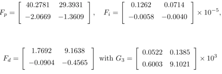
. Moreover, two first-order lags are included in the state to define the actuator dynamics. The angle of attack and the pitch angle are measured for the controller design. Therefore, the problem under consideration involves two inputs and two outputs along with six states. The two unstable eigenvalues of A are 0.6886± j0.2455. For this system, CB = 0, which implies that I + CB ¯Fd is always nonsingular. A feasible solution set is obtained through the ILMI algorithm with one iteration and the PID gains are obtained as follows: Fp= [ 40.2781 29.3931 −2.0669 −1.3609 ] , Fi= [ 0.1262 0.0714 −0.0058 −0.0040 ] × 10−5, Fd= [ 1.7692 9.1638 −0.0904 −0.4565 ] with G3= [ 0.0522 0.1385 0.6003 9.1021 ] × 103
One can compute that det(G3) = 3.9186× 10⁵̸= 0, which implies that the feasible solution set has been obtained with a nonsingular G3. The closed-loop eigenvalues of the system under static output feedback control
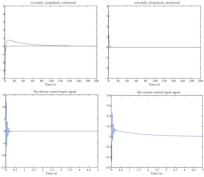
are calculated as −17.8284 ± j102.2630, −7.2104, −2.9999, −0.7169, −0.0256, which shows that the system is stabilized with the static PID output feedback control law of (15). The number of decision variables employed for this example is calculated as N oDV = 296 , while the number of decision variables used by He et al. [14] is computed as N oDV[14] = 201 . Moreover, Figures 3a and 3b depict the state trajectories of the linearized
open-loop aircraft system with u (t) = 0 showing that the unforced aircraft system is not asymptotically stable. When the static output feedback for the augmented system is applied, the state responses of the closed-loop system are exhibited in Figures 4a and 4b. Moreover, Figures 4c and 4d exhibit the elevon and the canard control input signals, respectively. As a result, the simulation results indicate that the closed-loop aircraft system is asymptotically stable under the proposed multivariable PID controller.
0 2 4 6 8 10 12 14 16 18 20 –18 –16 –14 –12 –10 –8 –6 –4 –2 0 2x 10 7 Time (s)
x1(solid), x2(dashed), x3(dotted)
0 2 4 6 8 10 12 14 16 18 20 –0.5 0 0.5 1 1.5 2 2.5 3x 10 6 Time (s)
x4(solid), x5(dashed), x6(dotted)
0 20 40 60 80 100 120 140 160 180 200 –4 –3 –2 –1 0 1 2 3 4 5 Time (s)
x1(solid), x2(dashed), x3(dotted)
0 20 40 60 80 100 120 140 160 180 200 –3 –2 –1 0 1 2 3 4 Time (s)
x4(solid), x5(dashed), x6(dotted)
0 0.5 1 1.5 2 2.5 3 3.5 4 4.5 5 –15 –10 –5 0 5 10 15 Time (s)
The elevon control input signal
0 0.5 1 1.5 2 2.5 3 3.5 4 4.5 5 –0.6 –0.4 –0.2 0 0.2 0.4 0.6 0.8 Time (s)
The canard control input signal
Figure 4. a) State trajectories of the closed-loop system. b) State trajectories of the closed-loop system. c) The elevon control input signal. d) The canard control input signal.
6. Conclusions
In this paper we have developed two new design methods: first a static output feedback stabilization and second multivariable PID controller design for unstable linear time-invariant systems via an iterative LMI optimization approach. The static output feedback control problem has been solved by introducing an iterative linear matrix inequality algorithm. A stabilizing static output feedback controller gain has been obtained iteratively by using a linear matrix inequality condition. The design of a multivariable PID controller has been considered with the idea of a transformation previously developed in the literature. The original linear time-invariant system with the multivariable PID controller has been represented as a static output feedback control system. The PID controller gains are obtained once the static output feedback control problem has been resolved through the use of the developed iterative LMI method. The proposed technique has been applied over two numerical examples. In particular, the illustration of the aircraft control application example has been shown to be quite significant. Simulation studies have also been conducted. The simulation results have shown that both the synthesized static
output feedback controller and multivariable PID controller perfectly stabilized the corresponding systems under consideration.
References
[1] Gu G. Stabilizability conditions of multivariable uncertain systems via output feedback control. IEEE T Automat Contr 1990; 35: 925-927.
[2] Trofino-Neta A, Kucera V. Stabilization via static output feedback. IEEE T Automat Contr 1993; 38: 764-765.
[3] Syrmos VL, Abdallah CT, Dorato P, Grigoriadis K. Static output feedback-a survey. Automatica 1997; 33: 125-137.
[4] Cao YY, Lam J, Sun YX. Static output feedback stabilization: An ILMI approach. Automatica 1998; 34: 1641-1645.
[5] Geromel JC, de Souza CC, Skelton RE. Static output feedback controllers: stability and convexity. IEEE T Automat Contr 1998; 43: 764-765.
[6] Cao YY, Sun YX, Mao WJ. A new necessary and sufficient condition for static output feedback stabilizability and comments on ‘Stabilization via static output feedback’. IEEE T Automat Contr 1998; 43: 1110-1111.
[7] Cao YY, Sun YX, Lam J. Simultaneous stabilization via static output feedback and state feedback. IEEE T Automat Contr 1999; 44: 1277-1282.
[8] Crusius CAR, Trofino A. Sufficient LMI conditions for output feedback control problems. IEEE T Automat Contr 1999; 44: 1053-1057.
[9] Wang Z, Burnham KJ. LMI approach to output feedback control for linear uncertain systems with D-stability constraints. J Optimiz Theory App 2002; 113: 353-372.
[10] Zheng F, Wang QG, Lee TH. On the design of multivariable PID controllers via LMI approach. Automatica 2002; 38: 517-526.
[11] Yu JT. A convergent algorithm for computing stabilizing static output feedback gains. IEEE T Automat Contr 2004; 49: 2271-2275.
[12] Fujimori A. Optimization of static output feedback using substitutive LMI formulation. IEEE T Automat Contr 2004; 49: 995-999.
[13] Lin C, Wang QG, Lee TH. An improvement on multivariable PID controller design via iterative LMI approach. Automatica 2004; 40: 519-525.
[14] He Y, Wang QJ. An improved ILMI method for static output feedback control with application to multivariable PID control. IEEE T Automat Contr 2006; 51: 1678-1683.
[15] Yoo DS, Chung MS. Performance improvement of output feedback control systems using the theory of variable structure systems. Electron Lett 1990; 26: 1210-1211.
[16] Wang C, Huang T. Static output feedback control for positive linear continuous-time systems. Int J Robust Nonlin 2013; 14: 1537-1544.
[17] Dong J, Yang GH. Robust static output feedback control synthesis for linear continuous systems with polytopic uncertainties. Automatica 2013; 49: 1821-1829.
[18] Safonov MG, Laub AJ, Hartmann G. Feedback properties of multivariable systems: The role and use of return difference matrix. IEEE T Automat Contr 1981; 51: 415-422.