Efficient Discovery of Join Plans in Schemaless Data
Aybar C. Acar
Department of Computer Engineering Bilkent University
06800 Ankara, Turkey
[email protected].
Amihai Motro
Department of Computer Science George Mason University
Fairfax, VA 22030 U.S.A.
[email protected].
ABSTRACT
We describe a method of inferring join plans for a set of relation in-stances, in the absence of any metadata, such as attribute domains, attribute names, or constraints (e.g., keys or foreign keys). Our method enumerates the possible join plans in order of likelihood, based on the compatibility of a pair of columns and their suitabil-ity as join attributes (i.e. their appropriateness as keys). We outline two variants of the approach. The first variant is accurate but poten-tially time-consuming, especially for large relations that do not fit in memory. The second variant is an approximation of the former and hence less accurate, but is considerably more efficient, allow-ing the method to be used online, even for large relations. We pro-vide experimental results showing how both forms scale in terms of performance as the number of candidate join attributes and the size of the relations increase. We also characterize the accuracy of the approximate variant with respect to the exact variant.
Categories and Subject Descriptors
H.2.4 [Database Management]: Systems—Relational databases; H.2.5 [Database Management]: Heterogeneous Databases
General Terms
Experimentation, Performance
Keywords
Dependency Inference, Join inference, Schema Matching
1.
INTRODUCTION
This paper considers the problem of inferring joins among rela-tional (tabular) data instances, in the absence of any metadata that describes the data. That is, given two or relations, determine if, and how, these relations should be joined, when no other information is available; e.g., the domains from which the relation columns are drawn, the labels of the columns, which columns are declared keys, which columns are governed by foreign key relationships, and so on.
Permission to make digital or hard copies of all or part of this work for personal or classroom use is granted without fee provided that copies are not made or distributed for profit or commercial advantage and that copies bear this notice and the full citation on the first page. To copy otherwise, to republish, to post on servers or to redistribute to lists, requires prior specific permission and/or a fee.
IDEAS2009, September 16-18, Cetraro, Calabria [Italy] Editor: Bipin C. DESAI
Copyright c2009 ACM 978-1-60558-402-7/09/09 $5.00
As a simple motivating example, consider the following two rela-tions retrieved from two different sources (e.g. a list of employees of ABC Corp. and the list of accounts at XYZ Bank):
Employees:
EmpID Name Phone 222-99-3034 Alice 555-3456 342-23-3244 Bob 555-3422 234-43-4322 Carol 555-3422 Accounts: SSN Tel Balance 222-99-3034 555-3456 $5644.03 342-23-3244 555-3422 $56.34 234-43-4322 555-3422 $3456.08
Immediate inspection by a human, even without any metadata, re-veals that there are two ways of joining these tables, namely joining with SSN = EmpID or Tel = Phone and one can see right away that the remaining seven combinations of these two relations will not succeed. Upon closer inspection it is apparent that SSN = EmpID is better way to join these two tables since we see that Bob and Carol have the same telephone number (meaning they share the same house/office line). Informally then, the aim of this paper is to simulate the same analysis in an automated manner without any descriptive information about the columns or known constraints. In a way the method proposed here acts as a simplified ad-hoc re-lational information integration system. Given a set of tables with no information about the columns and of how they are related to each other it attempts to find the most likely universal relation [19] with the given pieces. There are various applications that such an approach might find uses. The primary reason for the devel-opment this method has been as a tool in solution of the problem of query consolidation [1], which is the reversal of the information integration process by reassembling the components of a query de-composed to various sources by an information integrator, in or-der to estimate the original global query. Automatic join infer-ence between component results (which are not necessarily part of global schema) allows the query consolidation process to discover the global relation the user is interested in. This has uses such as finding trends in the demand for information and surveillance of suspicious information aggregation efforts.
Apart from query consolidation, a schema agnostic join inference method has appeal as a data source discovery and assimilation tool for unstructured or semi-structured sources [8], the most prominent of which is the World Wide Web. The sources on the Web that are exploitable by information integration systems currently are those with well defined access methods and rich metadata (e.g. XML based web services). There is however a large amount of informa-tion on the web which is published as tables with no such descrip-tive information. These include text documents with embedded ta-bles, web pages with HTML tables and even older text which has been scanned with OCR systems and put online. All of these doc-uments have tabular (i.e. relational) data that can be satisfactorily extracted from text automatically [24]. Even then, however, these are semi-structured data with no descriptions as to their meaning in a global schema or their dependencies. An automated join infer-ence method, if efficient, can analyze a large number of such pieces rapidly and find any possible join links between these and the ex-tensions of existing parts of a virtual database, thereby allowing them to be recruited to further increase the completeness of the information. Alternatively, the method proposed here can also be used as a data mining tool in its own right in collecting pieces of re-lational data strewn over multiple documents and joining them into larger, global relations that can then serve as fact tables or existing dimensions to fact tables in a data warehouse and can be mined for knowledge.
The first step in finding possible joins among unmarked relations is identifying the attributes that are compatible in their domains. As will be discussed in Section 2, there are various methods for matching attribute domains in previous literature. We will intro-duce a simpler method that is able to work with scarce informa-tion and in polynomial time by exploiting certain aspects of key attributes. Even when matching by domain is done, there may be multiple join paths available due to more than one pair of attributes matching. In order to solve this ambiguity, we make the assump-tion that likely joins paths are those that employ key-foreign key relationships among the relations. This is the reason that SSN = EmpID was considered as a more likely join in the above example, instead of matching telephone numbers. Given the data, employee IDs to Social Security Numbers present a perfect key-foreign key relationship. While it can be argued that there may be cases where interesting joins may be obtained by joining on non-key relation-ships we will limit ourselves in this paper to joins plans that are lossless, or if there are no such options to join plans that approxi-mate the same as much as possible.
As a second simplification on our approach, we limit our scope only to join plans that are minimal in the sense that they can always be processed as trees spanning the constituent relations. In other words, we only consider chain and star joins, including hybrids of these. Complete joins, where the join graph may include cycles are not considered due to the combinatorial intractability they cause. This simplification we feel is justified in order to arrive at an effi-cient method which can handle the more common join scenarios. Given these assumptions, our problem is then formally:
Assume there is a relation R0 such that a set of n relations R1...Rnapproximate the lossless join decomposition of R0.
Find a conjunctive constraint c such that σc(R1× R2× ... ×
Rn) is equivalent or maximally equivalent to R0. The the
terms of conjuct c are limited to equality constraints between pairs attributes of the different Ri
The terms in the conjunct are the equi-join links between pairs of relations. We thus need to find the set of links which are foreign key relationships such that all relations are connected in a single tree. If every input table is guaranteed to have at least one such good link to another table, then we can find the equivalent of R0. How-ever, given that the data coming from unstructured and independent sources is liable to be flawed both intensionally and extensionally, such perfect linkage is not guaranteed by any means. Thus we must be able to find the closest match, in other words the maximally equivalent with the available data. We approach this problem using an information theoretic measure by which we score each possible link between two relations with a value defining to what extent that link constitutes a foreign key relationship. Thereafter, the tree of links spanning all the input relations and having highest total score is the maximally equivalent one. Furthermore, we are able to rank alternative trees (i.e. join plans) by their total scores, thus achieving a method that has better recall.
Our work is described in two main sections. Section 3 describes in detail the exact and approximate methods for scoring join plans, and it analyses the computational cost of each. Section 4 discusses experimental results on the time performance of each method, and the accuracy of the approximate method. The paper concludes in Section 5 with a summary of the contributions and a brief discus-sion of further research directions. We begin in Section 2 with a review of relevant work.
2.
BACKGROUND
There are two major areas of research that are relevant to our prob-lem and the proposed solution. We initially review schema match-ing as it pertains to the matching of attribute domains. Subse-quently, we consider research on join inference and compare ex-isting methods with our approach.
2.1
Schema Matching
Schema matching is concerned with the reconciliation of two data-base schemas, and is of great importance in the area of information integration. The basic goal is to map elements of two schemas to each other. Generally, in the context of information integra-tion, one schema is the global schema of the virtual database and the other is that of a local source to be integrated. A comprehen-sive survey and classification of schema matching approaches are given in [25]. According to the classification done in that work, schema matching approaches vary according to whether they use intensional (schema-level) or extensional (instance-level) informa-tion. In other words, whether they match schemas on the basis of metadata only, or whether they also use the actual data in the repos-itories. Since in our case we assume no metadata, our approach is entirely extensional in nature.
Several instance-level schema matching approaches have been sug-gested. A good number of these are machine learning techniques to classify attributes as belonging to the same domain, including methods based on artificial neural networks [17], Bayesian infer-ence with feature selection [6], meta-learning [11], and rule based systems [9]. While many of these solutions are relevant to the first phase of schemaless join inference (attribute matching), they de-pend on learned generalizations about the domain of each attribute (i.e., the values commonly encountered). In our case, however, there is no “prior” information to train these learners on.
In the exact variant of our method, to be described in Section 3, we adopt a closed world assumption and assume the data we have
is all that exists. Therefore, while matching attributes domains we use a straightforward overlap measure. In the approximate method, where the complete data set cannot be processed efficiently, we use a constraint-based approach, in which attribute domains are matched on the basis of the syntax of the values rather than the values themselves. This is a simplified version of the algorithm de-scribed in [23] for inferring pattern matching finite automata from examples of text patterns — in our case a sample of values for the an attribute. Such constraint-based approaches have been used in schema matching methods [16] and include data types, cardinality, range and syntax.
2.2
Join and Dependency Inference
Relational query languages such as SQL were designed to unam-biguously retrieve a required set of tuples from databases of ar-bitrary size and complexity. However, such languages are by no means intuitive and generally require a steep learning curve. Fur-thermore, it is not generally possible for users to construct queries without knowing the schema of a database. Therefore, relational database systems and their associated query languages, while un-deniably useful, are ill-suited for use by the general public [10]. One of the main obstacles to usability has been identified as the difficulty of performing joins. This issue has been addressed for almost 30 years, in systems that can relieve users from having to specify these complicated query building operations explicitly. Possibly the first endeavour was the universal relation model [19], which attempts to make the joins among relations in a database transparent by automatically traversing the schema through join de-pendencies. There exists a problem of ambiguity, however, when the underlying schema graph contains cycles, and multiple lossless join paths can be constructed. The model was thus extended with the concept of maximal objects [18], which are expert-determined, meaningful partitions of the graph into acyclic subgraphs. Alter-natively, these maximal objects can be generated by analyzing the functional dependencies that exist among attributes. In cases where a query covers parts of more than one maximal object, the union is given as the result.
Another approach to the problem of identifying the join pattern de-sired by the user is to assign a cost to each possible join, and search for the join pattern with the lowest cost [27, 22]. The problem is reduced to computing a minimum cost directed Steiner tree. Later approaches to the problem deviate from earlier ones in that they do not attempt to find a single join or unify all possible joins. Inspired by how search engines work, newer methods discover mul-tiple solutions, and then rank them according to a relevance score which varies from study to study.
The Discover system, [13], uses keyword-based queries. The data-base is scanned to discover the keywords, and the relations that contain the keywords are connected through their primary-foreign key relationships. When several minimal join paths result, they are ranked according to the length of the join path, with shorter join sequences having more relevance. An improvement to this method was introduced in the DBXplorer system [2], which uses keyword indices (called symbol tables), to determine more efficiently the lo-cations of keywords in relations.
Another query interface, INFER [20], generates and ranks the top-kjoin possibilities and allows users to select the one intended
be-fore materializing the query. The results are ranked by prioritiz-ing shorter join sequences over longer ones and lossless joins over lossy joins. The generation of candidates in this system is partic-ularly efficient, according to the authors, in that it pre-computes the maximal join trees and looks up subtrees of these during query time.
Our approach to join inference falls is within this latter generation of methods, in that it ranks possible answers according to a rel-evance scheme. As we are interested in joining all the given rela-tions, ranking by join sequence length is not useful as in most cases all our join sequences are of the same length. Hence, our ranking scheme emphasizes the strength of the connections between vari-ous attributes of these relations and prioritizes spanning trees with higher total weights.
A more recent body related work pertains to the inference of func-tional and inclusion dependencies from completely schemaless or semi-schemaless data. By semi-schemaless we mean that, for ex-ample, the primary key may be known for each relation but the relationships of those keys to any foreign keys may be unknown. A pair of such papers [14, 7] describe two related methods (BHUNT and CORDS) which identify fuzzy and soft dependencies between columns. This is very similar to the method described in this pa-per. These approaches employ a rule-based approach based on histograms, and the χ2 test, respectively, while the present work makes use of the Kullback-Liebler Divergence metric for the same problem. All these approaches can compute the strength of a fuzzy dependency between a pair of columns, however we maintain that relative entropy is a better metric for multicolumn relationships. That is, given a question involving more than two columns: e.g. “In relation R(A,B,C), if column A functionally defines B with strength 0.9 and C with 0.8, how good a key of R is A ?”, the relative en-tropy metric can be used to compute a quantitatively meaningful answer to the question whereas other methods can only be used in a qualitative manner.
Other work, such as [4] and [5], describe rather efficient methods for identifying inclusion dependencies between columns. In identi-fying the strength of a join path, as will be seen in the next section, between two columns R.A and S.B on tables R and S, there are two factors. The first factor is the strength of the functional depen-dencies A → R and B → S, the second factor is the strength of the inclusion dependency R[A] ⊆ S[B]. As will be explained in the next section, our method computes the strength of both these fac-tors. In the exact version of the method we compute the strengths together whereas in the approximate method the strength of each factor is estimated separately and the strength of the join path is taken to be the product of these. The methods [4, 5] for computing inclusion dependencies can be substituted for the method described in Sec. 3.5 that approximates the strength of INDs1, however the strength of the FDs still have to be computed. For this, FD infer-ence methods such as those mentioned in the previous paragraph can be employed, instead of the information gain based method given in this paper. Our contribution is thus partly the proposal of fast alternatives for FD and IND inference methods. However, the primary contribution is the use of these measures to identify and rank the most likely join plans.
An important advantage of our approach that distinguishes it from
1
Later in the paper, the Di(Aj) coefficients used in Eqn. 3.5 aim
to approximate the strength of a possible soft inclusion dependency between columns Aiand Ajon different relations.
those described in the literature, is that it is completely schema-agnostic. Our system generates join plans for a given set of relation instances without any additional information, such as information on the domains of the attributes (or even their names), which at-tributes are keys, and any relationships (e.g., foreign key relation-ships) among these relations. Furthermore, it does not depend on any system catalog information (statistics such as cardinalities, do-main sizes, &c.). All of the previous work mentioned above de-pends on some or all of this information, as they are geared to-wards query optimization and processing in a single DBMS. Our approach, on the other hand, aims to find good join plans for re-lations pulled from possibly independent sources where a central schema or catalog is unavailable. In fact, our approach does not need a DBMS at all and can work directly on, e.g., flat files.
3.
METHODOLOGY
We assume an arbitrary number of relations R1, . . . , Rkthat need
to be joined. The arity of a relation R is its number of attributes; the cardinality of R is the number of its tuples and is denoted |R|. Given an attribute A of relation R, its set of distinct values is de-noted dom(A).
3.1
The Join Graph
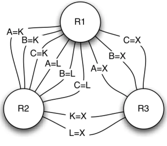
We model the input with an undirected and labeled multigraph G = (V, E), termed the join graph. The vertices V are the in-put relations R1, . . . , Rn, and the edges E are possible equi-joins
between the corresponding relations. As two relations could be joined on different pairs of attributes, there may be parallel edges and the edges are labeled with the join attributes. For example, an edge between vertices R1and R2labeled (A1, A2) represents
the equi-join R1 ./A1=A2 R2. Figure 1 shows an example join
graph involving three relations R1 = {A, B, C}, R2 = {K, L}
and R3 = {X} and a maximal set of edges, representing a
situa-tion where every pair of attributes from two different relasitua-tions is a possible equi-join.
R1
R2
R3
A=K
B=K
C=K
L=X
B=X
C=X
A=L
B=L
C=L
A=X
K=X
Figure 1: A join graph.
A join plan for the given relations is a relational algebra expres-sion in which every relation appears exactly once, and relations are connected with single-attribute equi-joins.2 In the example,
2
We assume that join plans do not have cycles, and that relations are joined with single attribute pairs. Composite join attributes can also be considered by ‘lumping’ subsets of attributes, without loss
R1 ./A=K R2 ./L=X R3 and R1 ./B=X R3 ./K=X R2 are
two join plans. Given a connected join graph, a join plan is repre-sented as a spanning tree.
Our goal is not merely to find a possible join plan, or to enumerate all the possible join plans. Rather, it is to sort the possible join plans according to their likelihood. Hence, we describe a method by which each join plan is assigned a likelihood score (a weight). An assumption that we make is that join plans are locally optimiz-able. That is, if given more than two relations, the most likely join plan is one that comprises the most likely individual joins. To achieve this, we describe a method for assigning weights to indi-vidual joins.
In the graph model, we score each edge in the multigraph with a weight that represents the likelihood of the join it represents. The weight of a join plan is then the sum of the weights of the partici-pating edges, and possible join plans are sorted by this total weight. The most likely join plan is the one that corresponds to a maximum weight spanning tree.
As an example, consider Figure 2, which shows a weighted version of the graph in Figure 1. For simplicity, only 5 of the 11 possible joins are considered. This simple join graph has a total of 8 possible spanning trees. Of these, the maximum spanning tree (shown in bold edges) denotes the join plan R1 ./B=K R2 ./L=X R3; The
tree in second place denotes the join plan R2 ./B=K R1 ./A=X
R3; and so forth.
R1
R2
R3
B=K
(0.9)
L=X
(0.6)
A=X
(0.3)
C=L
(0.2)
K=X
(0.1)
Figure 2: A weighted join graph.
Enumeration of spanning trees can be done by a variety of algo-rithms, and we use the algorithm by Kapoor and Ramesh [15], which allows the enumeration of an arbitrary number of spanning trees in order of total weight, and can handle multigraphs. Its com-of generality. However, one would then have to consider 2k− 1 instead of k possibilities for each k-relation. While certain heuris-tics based on value distributions might be available, the complexity of the general problem of discovering a minimal composite key has been shown to be NP-complete [12]. We therefore keep the treat-ment of join links between multiple-attributes out of the scope of this paper except to say that the method itself does not prevent in-ference of multi-attribute join plans provided that one is prepared to accept the increase in complexity.
plexity depends on the number of trees generated and the worst case complexity is O(N log V + V E), where V is the number of vertices, E is the number of edges and N is the desired number of top-ranked trees to be generated.
3.2
Pruning Edges
We now turn to the central issue of assigning weights to equi-joins. Given attribute A1of relation R1and attribute A2of relation R2,
we consider the join R1 ./A1=A2 R2 to be optimal (most likely),
if A1and A2have identical domains, and are primary keys of their
respective relations. The lesser the degree of satisfaction of these two conditions, the farther the join is from optimum.
To justify, consider the situations at the other extremes. (1) When the domains are completely disjoint, the join is empty; and (2) when the attributes are “anti-keys” (i.e., all tuples of R1 have the same
value in their A1attribute, and all the tuples of R2have the same
value in their A2 attribute), the join is either empty (when these
values are different), or the entire Cartesian product of R1 or R2
(when they are identical). In either of these extreme cases, the join R1./A1=A2R2is farthest from optimal.
The optimal join can be viewed as a foreign-key join, in which every tuple in one relation matches exactly one tuple in the other relation (a 1:1 matching). When the domains are not identical, there will be tuples in each relation that are not matched. And when the attributes are not strict keys, tuples in one relation may match several tuples in the other relation.
Hence, the likelihood of a join R1 ./A1=A2 R2 is derived from
these two parameters:
• The compatibility of dom(A1) and dom(A2).
• The selectivity of A1on R1, and the selectivity of A2on R2.
In a preliminary step, we identify those attributes that are consid-ered improbable as join atrributes. These include attributes that contain long character strings3or non-integers. These attributes are
discarded. Next, for the remaining attributes we construct a com-patibility matrix. Attribute comcom-patibility is calculated using this domain similarity measure:
sim(A1, A2) =
|dom(A1) ∩ dom(A2)|
|dom(A1) ∪ dom(A2)|
This values of this measure are between 0 and 1. The measure is 0 when the attributes are disjoint, and 1 when they are identi-cal. Using a threshold, the compatibility matrix is binarized. The join graph is then constructed with an edge for every two attributes judged compatible.
There is an anomaly that may occur in some join graphs that is cor-rected at this stage. As an example, consider a relation Country that
3In our experiments (to be detailed in the next section) we consider
attributes with strings exceeding 10 characters to be unlikely par-ticipants in joins. A threshold of 10 is arbitrary, albeit reasonable as 10 character alphanumeric strings would generally be sufficient as keys. Possible exceptions (e.g. URLs) exist and if such is known to be present in the data, this threshold can easily be increased or removed altogether. Clearly, while this pruning of certain columns is useful for performance, it has no effect on the rest of the method if omitted.
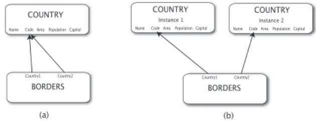
lists countries, and a relation Border that lists pairs of countries that share a border. In essence, Borders models a many-to-many rela-tionship between entities of Country. Figure 3(a) shows the initial join graph. Clearly, the desirable join plan is Country ./ Borders ./ Country, yet the spanning tree approach will not discover this join plan. This anomaly is rectified if the join graph includes two in-stances of Country, each with its own edge to Borders, as shown in Figure 3(b). In general, such situations are discovered by searching for edges from two different attributes of one relation to the same attribute of another relation. When such an occurrence is found, the vertex of the latter relation is split in two, with each vertex receiving one of the edges.
Name Code Area Population Capital
COUNTRY
Country1 Country2
BORDERS
Name Code Area Population Capital
COUNTRY
Instance 1
Country1 Country2
BORDERS
Name Code Area Population Capital
COUNTRY Instance 2
(a) (b)
Figure 3: Resolving join loops.
3.3
Weighting Edges
Having constructed a join graph based on attribute compatibility, we now describe how to score its edges on the basis of attribute selectivity. As mentioned earlier, our method quantifies the levels to which attribute relationships obey referential constraints. The method is based on the concept of entropy in information theory. The entropy of an attribute A is defined as
H(A) = X
v∈dom(A)
−p(A = v) log2p(A = v)
where p(A = v) is the proportion of tuples in which the value v occurs. Intuitively, H(A) measures the uniformity of the distribu-tion of the values of A. Assuming n distinct values, entropy ranges between 0 and log2(n). The maximal value corresponds to perfect
uniformity of distribution (lowest information content). For exam-ple, when dom(A) contains 4 distinct values, and each occurs 5 times, then H(A) = log2(4) = 2. In this case, H(A) is also the
number of bits required to represent the values of dom(A). Hence, entropy is measured in bits. We define the entropy of a relation R as the sum of the entropies of its attributes, i.e.
H(R) =X
i
H(Ai)
Let A be an attribute of R, and consider a “horizontal slice” of R, created by requiring A to have a specific value v. We denote the entropy of this slice H(σA=v(R)). As dom(A) is the set of all the
values of attribute A, its values partition R to several such slices, each with its entropy. We average these slice entropies with their expected value. The new value reflects the entropy of R when the values in A have been specified. We term this the posterior entropy of R given the attribute A:
H(R|A) = X
v∈dom(A)
p(A = v)H(σA=v(R))
The posterior entropy reflects a reduced level of uncertainty when R has been partitioned by its A values. The difference between
the prior and posterior entropies quantifies this reduction. For a meaningful comparison with reductions obtained in other relations using other attributes, we normalize this difference by dividing it by the prior probability. We term the result the information gain in R given attribute A:
I(R|A) = H(R) − H(R|A) H(R)
Assume A1is attribute of relation R1and A2is attribute of relation
R2, and consider the join R1 ./A1=A2 R2. For each tuple of R1
the value of A1is compared to the value of A2in each tuple of R2.
dom(A1) ∩ dom(A2) is then the set of values of A1 that find a
match in R2. Therefore, in the aftermath of the join, the relation
A2is partitioned by the values in the set dom(A1) ∩ dom(A2).
The information gain of R2in the aftermath of this join is therefore
I(R2|A2) =
H(R2) − H(R2|A2)
H(R2)
(1) Note that the posterior entropy H(R2|A2) is calculated as the
ex-pected values of entropies for slices created by values in dom(A1)∩
dom(A2).
If A2 is a key of R2, then each of the slices has a single tuple.
Therefore each of the slice attributes contains just one value and its entropy is 0. Since slice entropy is the sum of its attribute entropies, each slice entropy is 0. Consequently, the posterior entropy of R2
is 0, as well, and the information gain of R2in the aftermath of the
join is 1.
If A2 is anti-key (dom(A2) has but a single value), then a single
slice is created, the posterior entropy of R2is the same as its prior
entropy, and the information gain in the aftermath of the join is 0. In between these extreme cases, the information gain is a value be-tween 0 and 1. The information gain will be higher when slice sizes are more uniform, and the tuples in each slice are more homoge-neous. In other words, the more an attribute acts like a key, the closer its gain will be to 1.
This method may be regarded as an information theoretic way of quantifyingreferential constraints. If a foreign attribute produces an information gain of 1 in another relation, that relation is func-tionally dependenton the attribute. Indeed, this approach general-izes the definition of dependency from a binary concept to a gradual one.
Note, however, that the join operation is symmetrical, and thus in-duces a dual information gain in R1:
I(R1|A1) =
H(R1) − H(R1|A1)
H(R1)
The weight assigned to the edge that denotes the join R1./A1=A2
R2is therefore a pair of values, expressing the information gain of
each of the join participants:
w(A1, A2) = (I(R1|A1), I(R2|A2))
When ranking spanning trees we use the higher of the two values to decide between two different edges; the second value is used to resolve ties.
3.4
Cost Analysis
To help analyze the cost of our method for assigning weights to the edges of a join graph, Figure 4 summarizes the method in algorithm format. In this figure, the set Candidates accumulates the edges that pass the compatibility test, and θ is the threshold of compatibility.
1: Candidates ← ∅ 2: for all Aido
3: if Aiis a viable join attribute then
4: Candidates ← Ai
5: end if 6: end for
7: for all Ai∈ Candidates do
8: for all Aj∈ Candidates do
9: if i 6= j and Aiand Ajare in different relations then
10: if sim(Ai, Aj) < θ then 11: Discard edge (Ai, Aj) 12: else 13: Calculate w(Ai, Aj) 14: end if 15: end if 16: end for 17: end for
Figure 4: Pruning and weighting.
Let K denote the total number of relations, P the average arity, and N the average cardinality. Typically, K and P are small, whereas N could be very large. The initial pruning phase (lines 1–6) can be done by a single pass of each relation, and is therefore of complex-ity O(KN ).
The calculation of similarity of two attributes (line 10) requires finding the cardinality of the union and intersections of the two domains. This can be accomplished by sorting the two relations on these attributes and then traversing both relations simultaneously. The time required for calculating a single similarity is therefore of complexity O(N log N ).
The calculation of weights (line 13) is slightly more complicated. Consider the join R1 ./A1=A2 R2. First, each relation is sorted
on its join attribute. Next, R1is traversed, and for each new value
of A1, the matching tuples of R2 (if any) are written out. These
constitute a slice. To calculate the posterior entropy of this slice, it is sorted P times; after each sort, the slice is traversed and the posterior entropy of one attribute is calculated. Eventually, the pos-terior entropy of the slice is derived by summation. The number of slices is V = dom(A1) ∩ dom(A2) and each slice has on average
N/V tuples. Hence, the total cost is 2N log N for the sorts, 2N for the traversals, and V P ((N/V ) log(N/V ) + N/V ) for sorting and traversing each of V slices P times. Hence, the cost of calcu-lating the posterior entropy H(R2|A2) is at worst O(P N log N ).
Calculating the prior entropy H(R2) is done by P sorts and
traver-sals, with cost O(P N log N ). Altogether, the calculation of each information gain is of complexity O(P N log N ).
To estimate the cost of the entire algorithm we add the cost the initial pruning and the cost of calculating similarity and weights for every pair of attributes from different relations. At worst, there will be P2K2 such pairs.4 Altogether, the cost of generating the weighted join graph is O(P3K2N log N ).
4Note that each edge requires two calculations, one for each of its
3.5
Optimization
Clearly, the most time consuming steps of the algorithm are the cal-culations of sim(Ai, Aj) and w(Ai, Aj). This computational task
may be reduced by using a Monte Carlo approach. Instead of using the complete relations Riwe use subsets R0iobtained by random
samples. From each sample of a relation, we obtain a sample of each of its attributes by a projection. Random samples relation can be done in O(N ) time (a single pass of each relation is required). Assuming our sampling rate |R0i|/|Ri| is such that the samples can
fit into memory, we will be able to perform these two computations quickly.
However, calculating sim(Ai, Aj) on samples presents problems.
For example, assume Aiand Ajare key attributes and dom(Ai) =
dom(Aj). Even when sampling as much as half of the domains,
we could not guarantee a match. We address this problem by us-ing classifiers to summarize domains. As discussed in the related work, several classifiers have been proposed to match domains of attributes. Most of these are general in nature and relatively expen-sive to train. In our case, however, the domains of attributes that survived the initial pruning step have certain helpful characteris-tics.
Join attributes are generally either integers or short strings of char-acters (or a combination of these); for example, ID numbers, tele-phone numbers, model numbers, geographic locations, and dates. Such values are often described by simple regular expressions. We therefore summarize our domains by representing them as small fi-nite automata that recognize the strings in a domain. For example, the domain of US Social Security numbers of the form 123-45-6789 may be summarized as the regular expression {d3-d2-d4}5
. To accomplish this, we use the ID algorithm proposed by Angluin [3] which gives a canonical deterministic finite automaton (DFA) that will recognize a set of strings. The complexity of the algorithm is O(N P |Σ|), where N is the number of states, P is the size of the training set, and |Σ| is the size of the alphabet. A simple alphabet that can be used is one that includes one symbol for all letters, one symbol for all digits, and several symbols for punctuation marks. The number of states in the DFA cannot be larger than the size of the alphabet times the longest string in the language. Since our alphabet is small and the strings in our domains are small as well, both |Σ| and N are small with respect to P . Thus, we can bound the complexity of creating a DFA to O(P ). Recall that P is the size of the training set, namely the size of our sample.
Let A01 and A02 be samples of dom(A1) and dom(A2),
respec-tively. Based on these samples we construct two DFAs, denoted D1and D2, respectively, to recognize these domains. Given a set
of strings S, let Di(S) denote the proportion of strings recognized
by Di. We now define a new similarity measure to quantify the
compatibility of two domain samples A01 and A 0
2. D1(A02)
mea-sures the level to which a DFA trained to recognize A01recognizes
the set A02. Hence, it can be viewed as measuring the similarity
of A02 to A 0
1. In duality, D2(A01) quantifies the level to which a
DFA trained to recognize A02recognizes the set A 0
1. Hence, it can
be viewed as measuring the similarity of A01 to A02. These two
“directional” similarity measures are multiplied to create the new measure of similarity, denoted sim0:
sim0(A01, A 0 2) = D1(dom(A 0 2)) · D2(dom(A 0 1)) 5Assume the subset d of the alphabet matches any digit (i.e. 0-9)
and the ’-’ matches a dash.
The new measure, which is calculated on domain samples, will be used to measure the compatibility of the domains.
The other costly calculation is that of information gain (which pro-vide the weights). Here, too, we can define approximate informa-tion gain. Equainforma-tion 1 expressed the informainforma-tion gain of R2in the
aftermath of a join R1 ./A1=A2 R2. Instead of using the entire
relation R, we could use a sample R0of R, and define approximate information gain: I0(R02|A 0 2) = H(R02) − H(R02|A02) H(R0 2) We then use I0(R02|A 0
2) to estimate I(R2|A2). Because we are
working with samples, the time required to calculate the estima-tion is much smaller than the time required to calculate the actual information gain.
Recall, however, that the calculation of H(R2|A2) used only the
values of dom(A2) that are present in dom(A1). Hence, when
working with samples, we need to calculate dom(A01) ∩ dom(A 0 2).
But, as discussed earlier in this subsection, approximating the inter-section of domains with the interinter-section of samples is not a viable option.
For a moment, assume that the two domains are identical. Then dom(A01) ∩ dom(A
0
2) = dom(A 0
2), and we could use dom(A 0 2)
(no need to intersect). Since this assumption cannot be made safely, we correct the information gain obtained by multiplying it by the selectivity of the DFA for recognizing dom(A02) as it is applied to
dom(A01) (i.e., we reduce the information gain by the same factor
that D1would have reduced dom(A02)). Altogether we obtain this
estimator for the weight pair: w0(A1, A2) = (I 0 (R01|A 0 1) · D1(A 0 2), I 0 (R02|A 0 2) · D2(A 0 1))
Notice that D1(A02) is an approximation of the inclusion
depen-dency A1 ⊆ A2. D1(A02) = 1 when there is a perfect IND
be-tween the attributes. Likewise, I0(R01|A01) is an approximation
of the strength of the FD A1 → R1. Thus, the product of these
terms, along with the product of the symmetric terms D1(A02) and
I0(R02|A02) gives the estimated strength (i.e. the lossless-ness) of
the join path R1./A1=A2R2.
The new calculation has two advantages with respect to complex-ity. First, the entire process is performed on a sample of N (which is often an order of magnitude smaller). Second, and more signif-icant, is the number of times that similarity and weight are calcu-lated. This is due to the fact that the need to intersect domains has been removed from both of these calculations. Previously, a given attribute Ajin relation Rineeded to be compared with each of the
P attributes of each of the other relations, essentially P K times. Since the calculations now are essentially independent of the other attributes (for example, the new information gain of Ri.Ajis
calcu-lated just once, and only corrected for each counter-attribute Rk.Al
by the acceptance rate of the latter domain by the DFA of the former domain, which is also calculated just once), the new complexity is only O(P2KS log S), where S is the sample size. As the exper-iments described in the next section demonstrate, this reduction is very significant.
4.
EXPERIMENTATION
To validate the cost analysis of the previous section and to measure the accuracy of the approximate method, we conducted a series of experiments. The TPC-H [26] benchmark database was used for testing both the time performance of the exact method and the accuracy and performance of the approximate (sampling) variant. The database management system used is MySQL 5.1. In the exact method, the DBMS is used extensively to calculate domain overlap and to determine the weights of join candidates. The approximate method begins by randomly sampling a small subset of each rela-tion into memory and thereafter works entirely in memory. Ran-dom sampling requires one scan of each relation and thus database access (i.e., disk access) is only linearly dependent on the size of the given relation.
Since performance measures are given as absolute times (i.e., in seconds and milliseconds), one must be aware of the computing en-vironment: All experiments were performed on a 2.3GHz dual-core x36 processor with 2GB of memory, using the OS X 10.4 operating system. The implementation was done in Java. The execution of the program was locked into one of the cores of the CPU with the system and DBMS making use of the other core when necessary.
4.1
Performance
The exact method was tested for performance by analyzing a pos-sible join of a relation from the TPC-H database with itself. We chose the LineItem relation, which is the largest, both in the num-ber of rows and columns. This is a worst-case test of the method since when a relation is joined with an identical copy, every column matches at least one other column in the counterpart. We tested with various horizontal and vertical subsets of the relation, includ-ing subsets with 100, 500, 1000, 1500, 2000, 2500 and 3000 rows, each with 2, 3 and 4 joinable attributes. Each of the 21 scenarios was carried out 20 times each to average the time required. The DBMS query cache was flushed after each run to avoid deceptively fast performance. The times required to generate the weighted join graph (in this case, a bipartite graph since there are just two rela-tions) between the two relations are given in Figure 5. Each of the 21 points represents the mean time of the 20 experiments, and the range bars represent standard deviation. The shape of each point corresponds to the number of columns (P ).
0 500 1000 1500 2000 2500 3000
Relation size (number of tuples)
0 50 100 150 200 250 300
Run time (sec)
P = 2 (R = 0.99993) P = 3 (R = 0.99981) P = 4 (R = 0.99962)
Figure 5: Running times of the exact method. The results show that the exact method is too costly in situations
where either the arity or the size of the relations are considerable. Recall from the previous section that the growth with respect to size is weaker (N log N ), whereas the growth with respect to the average arity is cubic in the worst case (P3). Notice that, since we are experimenting with join plans involving two identical relations, the number of relations (K) is fixed at two, but in general the exact grows quadratically growth with the number of relations.
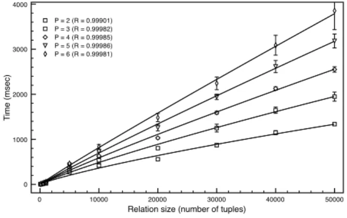
In contrast, the approximate method is several orders of magnitude faster and scales much more favorably with respect to all these pa-rameters. To bear this out, we repeated the previous experiment but with different relation sizes. The relation was again LineItem, with a total of 100,000 rows. We performed the experiments with sam-pling rates of 0.001, 0.01, 0.05, 0.1, 0.2, 0.3, 0.4 and 0.5.6 Each of the 21 scenarios was run 100 times. The largest arity (P ) used was 6.7Some of the 6 columns were then removed to test the effect of the arity. An approximate method run begins with a pseudo-random sampling of the original relaation for the required sample size. The MT19937 variant of the Mersenne Twister PRNG is used and the generator is seeded with the system timer at the beginning of each run. The rest of the operation is conducted completely in memory. This includes finding domain matches through the induc-tion of simple pattern matching DFAs and the calculainduc-tion of the conditional entropy of the relation given each attribute.
Figure 6 shows the mean time for each scenario. The data points of each arity were fit with functions of the form a + bx log(cx) to indicate the expected scaling with respect to sample size. Notice that even with large sample sizes (e.g., 10,000 rows obtained with a 0.1 sample rate) the operation is fast enough to be completed in less than a second using modest hardware. Moreover, since the cal-culations for each attribute could be done separately, a production system could use multiple processors in parallel, to obtain almost linear speedup, thus allowing real-time operation. In Section 4.2 we show that this sampling rate is sufficient to accurately predict join rankings.
0 10000 20000 30000 40000 50000
Relation size (number of tuples) 0 1000 2000 3000 4000 T ime (msec) P = 2 (R = 0.99901) P = 3 (R = 0.99982) P = 4 (R = 0.99985) P = 5 (R = 0.99986) P = 6 (R = 0.99981)
Figure 6: Running times of the approximate method. The scaling of computation time with respect to the number of pos-sible join attributes was further investigated. As none of the re-lations in the TPC-H benchmark database contains more than 16
6
This corresponds to sample sizes of 100, 1000, 5000, 10000, 20000, 30000, 40000 and 50000 rows, respectively
7
Although the relation has 16 columns, only 6 of them satisfy the requirement that equi-join attributes be either integers or short strings.
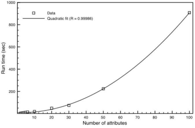
attributes, a synthetic relation of 50,000 rows and 100 attributes was generated. The relation was such that every attribute is a key and each attribute is domain-compatible with every other attribute. Hence, when the relation is joined with itself, the method is forced to consider a complete join graph.
10 20 30 40 50 60 70 80 90 100 Number of attributes 200 400 600 800 1000
Run time (sec)
Data
Quadratic fit (R = 0.99986)
Figure 7: Running times of the approximate method with dif-ferent numbers of join attributes.
Figure 7 shows the results of this simulation. The simulation was run once for various projections of different arity. The resulting data was fitted with a quadratic function, which is shown as well. As predicted by the analysis, the approximate method grows in a quadratic manner with the number of possible join attributes. Note, however, that the quadratic nature is not very pronounced for arities less than 10. Therefore, for relations of arity less than 10, the per-formance should not be affected. Due to database normalization and the human attention span8 it is uncommon for relations used directly by human users to have an exceedingly large number of attributes and the candidate join attributes will be fewer yet.
4.2
Accuracy
The exact method considers all the tuples of a relation, and scores the plausibility of each possible join between every pair of rela-tions. This method also finds exact domain overlaps by intersecting complete tuple sets. The approximate method atempts to estimate the same by using only a fraction of the tuples of each relation. Fur-thermore, the calculation on each relation is independent of other relations.
As shown, the approximate method performs impressively. How-ever, its accuracy — the degree to which it correctly approximates the full calculation — requires investigation. We tested the accu-racy of the approximate method using the exact method as a stan-dard.
The weights assigned by the approximate method to each edge in the join graph consist of two distinct values. The first value denotes the extent to which the domains of the attributes at each end of the
8
The human cognitive channel limits the number of items that can be retained by the average user at about 7 [21]. Of course, with automated queries this number can be significantly larger. How-ever, the main aim of this study is to find likely join plans in a query consolidation system [1], and the assumption is that most of the queries will be ad-hoc constructs built by humans and hence subject to human limitations.
edge match each other. This is determined by classifying the do-main of one sampled attribute with a DFA trained on the dodo-main of the other. The second value denotes the extent to which either attribute serves as a key to its own relation. This is done by calcu-lating the prior entropy of the sampled relation and the conditional entropy of that relation given the attribute, and then calculating the relative change (the information gain). Since we are trying to esti-mate this statistic based on a sample of the complete relation, the accuracy of the method depends primarily on the relative size of the sample. 0 0.2 0.4 0.6 0.8 Sampling ratio 0 0.1 0.2 0.3 0.4 0.5
Relative error in assigned weights
Figure 8: Error in Weights Assigned by the Sampling Method with respect to the Exact Method
In order to investigate the effects of varying sample size on accu-racy we experiment on the system in a bottom up fashion, starting with the error in individual edge weights and working up to the ranking of join plans. Figure 8 shows the error in weighting of edges with varying sampling rates. The weighting error for any edge < A1, A2> is defined as:
E(A1, A2) =
|wexact(A1, A2) − wapprox(A1, A2)|
wexact(A1, A2)
Each point in the figure is thus the mean weighting error for all edges in pairwise join inferences between tables in the TPC-H data-base. The error bars represent the standard deviation in the weight-ing error. This variance is negligible in cases where the sample size is more than 5% of the total relation. Hence, as long as the sample size is within an order of magnitude of the original relation, the be-havior of the approximate method is stable enough to be considered to be deterministic.
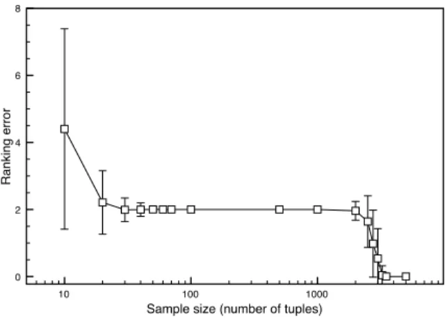
Figure 9 shows the effects of the weighting error on ranking. The LineItem table in the TPC-H was experimented on in order to be able to consistently compare ranking of the exact method and the approximate variant. The experiments were done on a pair of ta-bles. Since the method we use is locally optimized, if the links between every pair of tables is weighted correctly the whole join graph is assumed to be correctly weighted. Therefore, without loss of generality we focus our experimentation to pairwise weighting between tables. In this case, there are 12 possible edges in the join graph and the original relation has 100000 rows. The exact method was run once to find the benchmark ranking. Subsequently, the ap-proximate method was run 20 times each at various sample sizes
and made to rank the same 12 edges. The figure shows the mean ranking error as the sample size increases. The error bars represent the standard deviation. Even at samples of 70 rows (i.e. a sam-ple less than 1% of the original.), the ranking of the approximate method stabilizes at a ranking error of 2 (i.e. each edge is ranked on average two places away from their position in the benchmark ranking). As the sample size becomes large enough to comprise a fraction of the original relation (e.g. 20% of the whole) the ranking of the approximate method converges to that of the exact method.
10 100 1000
Sample size (number of tuples)
0 2 4 6 8 Ranking error
Figure 9: Average Error in Candidate Join Rank of the Sam-pling Method with respect to the Exact Method
Therefore, for normally or uniformly distributed tables, the approx-imate method is able to pick out distinctly better join plans and rank them at the top, even when the sample taken is one hundredth of the total population. However, it is difficult for the method to differ-entiate the more ‘mediocre’ join plans without more information. This is clearly seen in 9 the initial inflection at around a sample size of 50 represents the point where the most promising joins have settled in the top ranks. This is where we have actually discovered what the most plausible join is. As the sample size, and hence the information available to the method, increases even the lower rank-ings converge to the correct ranking. This is seen as the second inflection in the figure at around a sample size of 2000 (i.e. a 20% sample). Figure 10 further illustrates this effect. At the former in-flection, the top join plan has stabilized and is thereon consistently found as the top join. After the second inflection, all rankings are consistently the same with the benchmark ranking (denoted as the percentage of ‘perfect rankings’ in the figure). Therefore the ap-proximate method can consistently find the top ranked join plans at 1% sample size and is virtually the same as the exact method for sample sizes above 20%.
5.
CONCLUSION
We introduced a new approach to inferring join plans amongst a number of relations in the absence of any metadata. The method ranks spanning trees over a join graph, each spanning tree over be-ing join a possible join plan. We approach this problem by weight-ing each of the edges in the graph (i.e., each possible equi-join) with a score based on the information gain given the join. We then rank these possible spanning trees in order of decreasing weight. There are two forms of the method discussed. The former variant is exact in that it calculates the information gain over each of the participant relations given the set of values in the join attribute of
10 100 1000
Sample size (number of tuples)
0 20 40 60 80 100 Percent of runs
Top join correct Perfect ranking
Figure 10: Accuracy of the Total Ranking of the Sampling Method with respect to the Exact Method
the other. While this correctly evaluates both selectivity join and attribute domain matching, it requires pairwise processing of every pair of relation and is expensive to compute. The optimized variant of the approach computes the information gain on a relation given its own candidate join attribute and furthermore performs this on a smaller sample of the relation. Thus, each relation can be pro-cessed by itself. However, this only computes the selectivity of the candidate join and not the attribute compatibility with the attributes of other relations. Therefore, this weight is corrected by the result of a domain matching approach that uses the syntax of the values to determine compatibility.
We have shown in experiment that the approximate approach is several orders of magnitude faster and scales more favorably (i.e., quadratic vs log-linear). Furthermore, experimentation has shown that in terms of accuracy, the optimized method is virtually equiva-lent in ranking to the exact one at sample sizes that are 20-25 % of the whole relation. Even with considerably smaller samples (e.g., 1 %) the approximate method can identify the most likely join plans and ranks them at the top.
The methods given in this paper assume that the joins are done on a single attribute between any two relations. In real world applica-tion, while not as likely, there are many instances of joins needing a combination of two or more fields. While the current method can be extended to multiple attribute join keys without loss of general-ity, the time performance in such a setting will suffer. Part of our future work is making the approach applicable to multiple attribute joins without unnecessary loss of performance. Another possible improvement is the addition of support for cyclic joins. As it stands, the use of spanning trees to represent join plans precludes the possi-bility of inferring a cyclic join. While not as common as chain and star joins, cyclic joins will nevertheless be an interesting addition to the current approach.
6.
REFERENCES
[1] A. C. Acar and A. Motro. Query Consolidation: Interpreting a Set of Independent Queries Using a Multidatabase Architecture in the Reverse Direction. In Proc. of the International Workshop on New Trends in Information Integration, VLDB’ 09, pages 4–7, 2008.
Keyword Search over Relational Databases. In Proc. of ICDE ’02, pages 5–16, 2002.
[3] D. Angluin. A Note on the Number of Queries Needed to Identify Regular Languages. Information and Control, 51(1):76–87, 1981.
[4] J. Bauckmann, U. Leser, F. Naumann, and V. Tietz. Efficiently Detecting Inclusion Dependencies. In Proc. of ICDE ’07, pages 1448–1450, 2007.
[5] S. Bell and P. Brockhausen. Discovery of Data Dependencies in Relational Databases. Technical report, Universitat Dortmund, 1995.
[6] J. Berlin and A. Motro. Database Schema Matching Using Machine Learning with Feature Selection. In Proc. of CAiSE 02, pages 452–466, 2002.
[7] P. G. Brown and P. J. Haas. BHUNT: Automatic Discovery of Fuzzy Algebraic Constraints in Relational Data. In Proc. of VLDB ’03, pages 668–679, 2003.
[8] P. Buneman. Semistructured Data. In Proc of PODS ’97, pages 117–121, 1997.
[9] S. Castano and V. De Antonellis. A Schema Analysis and Reconciliation Tool Environment. In Proc. of IDEAS ’99, pages 53–62, 1999.
[10] T. Catarci. What Happened When Database Researchers Met Usability. Information Systems, 25(3):177–212, May 2000. [11] A. Doan, P. Domingos, and A. Halevy. Reconciling Schemas
of Disparate Data Sources: A Machine Learning Approach. In Proc. of SIGMOD ’01, pages 509–520, 2001.
[12] D. Gunopulos, R. Khardon, H. Mannila, S. Saluja, H. Toivonen and R. S. Sharma. Discovering All Most Specific Sentences. ACM Transactions on Database Systems, 28(2):140–174, 2003.
[13] V. Hristidis and Y. Papakonstantinou. DISCOVER: Keyword Search in Relational Databases. In Proc. of VLDB ’02, pages 670–681, 2002.
[14] I. F. Ilyas, V. Markl, P. Haas, P. Brown, and A. Aboulnaga. CORDS: Automatic Discovery of Correlations and Soft Functional Dependencies. In Proc. of SIGMOD ’04, pages 647–658, 2004.
[15] S. Kapoor and H. Ramesh. Algorithms for Enumerating All Spanning Trees of an Undirected Graph. SIAM Journal on Computing, 24(2):247–265, 1995.
[16] J. Larson, S. Navathe, R. Elmasri, and M. Honeywell. A Theory of Attributed Equivalence in Databases with Application to Schema Integration. IEEE Transactions on Software Engineering, 15(4):449–463, 1989.
[17] W. Li and C. Clifton. SEMINT: A Tool for Identifying Attribute Correspondences in Heterogeneous Databases using Neural Networks. Data & Knowledge Engineering, 33(1):49–84, 2000.
[18] D. Maier and J. D. Ullman. Maximal Objects and the Semantics of Universal Relation Databases. ACM Transactions on Database Systems, 8(1):1–14, 1983. [19] D. Maier, J. D. Ullman, and M. Y. Vardi. On the Foundations
of the Universal Relation Model. ACM Transactions on Database Systems, 9(2):283–308, 1984.
[20] T. Mason and R. Lawrence. INFER: A Relational Query Language without the Complexity of SQL. In Proceedings of CIKM ’05, pages 241–242, 2005.
[21] G. A. Miller. The Magical Number Seven, Plus or Minus Two: Some Limits on Our Capacity for Processing Information. Psychological Review, 63(2):81–97, 1956.
[22] A. Motro. FLEX: A Tolerant and Cooperative User Interface to Databases. IEEE Transactions on Knowledge and Data Engineering, 2(2):231–246, 1990.
[23] R. Parekh and V. Honavar. An Incremental Interactive Algorithm for Regular Grammar Inference. In Proc. of ICGI 96, 1996.
[24] D. Pinto, A. McCallum, X. Wei, and W. Croft. Table Extraction using Conditional Random Fields. In Proceedings of SIGIR ’03, pages 235–242, 2003.
[25] E. Rahm and P. A. Bernstein. A Survey of Approaches to Automatic Schema Matching. The VLDB Journal, 10(4):334–350, 2001.
[26] Transaction Processing Performance Council. TPC Benchmark H Rev 2.6.1. Standard Specification, 2007. [27] J. A. Wald and P. G. Sorenson. Resolving the Query
Inference Problem using Steiner Trees. ACM Transactions on Database Systems, 9(3):348–368, 1984.