Computational study of power conversion and luminous efficiency performance for semiconductor quantum dot nanophosphors on light-emitting diodes

(1)

Computational study of power conversion and

luminous efficiency performance for

semiconductor quantum dot nanophosphors on

light-emitting diodes

Talha Erdem,1 Sedat Nizamoglu,1 and Hilmi Volkan Demir1,2,*

1_{Department of Electrical and Electronics Engineering, Department of Physics, and UNAM–Institute of Materials} Science and Nanotechnology, Bilkent University, Ankara, 06800, Turkey

2

School of Electrical and Electronic Engineering, School of Physical and Mathematical Sciences, Nanyang Technological University, Singapore 639798, Singapore

*volkan@stanfordalumni.org

Abstract: We present power conversion efficiency (PCE) and luminous

efficiency (LE) performance levels of high photometric quality white LEDs integrated with quantum dots (QDs) achieving an averaged color rendering index of ≥90 (with R9 at least 70), a luminous efficacy of optical radiation

of ≥380 lm/Wopt a correlated color temperature of ≤4000 K, and a

chromaticity difference dC <0.0054. We computationally find that the

device LE levels of 100, 150, and 200 lm/Welect can be achieved with QD

quantum efficiency of 43%, 61%, and 80% in film, respectively, using state-of-the-art blue LED chips (81.3% PCE). Furthermore, our computational analyses suggest that QD-LEDs can be both photometrically and electrically more efficient than phosphor based LEDs when state-of-the-art QDs are used.

OCIS codes: (160.4670) Optical materials; (160.4760) Optical properties; (230.3670)

Light-emitting diodes; (230.5590) Quantum-well, -wire and -dot devices.

References and links

1. Energy Savings Estimates of Light Emitting Diodes in Niche Lighting Applications, Building Technologies Program, Office of Energy Efficiency and Renewable Energy, U.S. Department of Energy (2011).

2. J. M. Phillips, M. F. Coltrin, M. H. Crawford, A. J. Fischer, M. R. Krames, R. Mueller-Mach, G. O. Mueller, Y. Ohno, L. E. S. Rohwer, J. A. Simmons, and J. Y. Tsao, “Research challenges to ultra-efficient inorganic solid-state lighting,” Laser Photon. Rev. 1(4), 307–333 (2007).

3. S. Nizamoglu, T. Erdem, X. W. Sun, and H. V. Demir, “Warm-white light-emitting diodes integrated with colloidal quantum dots for high luminous efficacy and color rendering,” Opt. Lett. 35(20), 3372–3374 (2010), http://www.opticsinfobase.org/abstract.cfm?uri=ol-35-20-3372.

4. M. R. Krames, O. B. Shchekin, R. Mueller-Mach, G. O. Mueller, L. Zhou, G. Harbers, and M. G. Craford, “Status and future of high-power light-emitting diodes,” J. Disp. Technol. 3(2), 160–175 (2007). 5. DEMA Electronic AG, http://www.zenigata.de (accessed on August 17, 2011).

6. Cree Inc, http://www.cree.com/press/enlarge.asp?i=1174480795673 (accessed on August 17, 2011). 7. OSRAM Opto Semiconductors GmbH,

http://www.osram- os.com/osram_os/EN/Press/Press_Releases/Solid_State_Lighting/2011/From_the_OSRAM_laboratory_-_efficiency_record_for_warm_white.html (accessed on August 17, 2011).

8. O. Graydon, “The new oil?” Nat. Photonics 5(1), 1 (2011).

9. T. Erdem and H. V. Demir, “Semiconductor nanocrystals as rare-earth alternatives,” Nat. Photonics 5(3), 126 (2011).

10. T. Erdem, S. Nizamoglu, X. W. Sun, and H. V. Demir, “A photometric investigation of ultra-efficient LEDs with high color rendering index and high luminous efficacy employing nanocrystal quantum dot luminophores,” Opt. Express 18(1), 340–347 (2010), http://www.opticsinfobase.org/oe/abstract.cfm?URI=oe-18-1-340.

11. K. Sanderson, “Quantum dots go large,” Nature 459(7248), 760–761 (2009).

12. E. Jang, S. Jun, H. Jang, J. Lim, B. Kim, and Y. Kim, “White-light-emitting diodes with quantum dot color converters for display backlights,” Adv. Mater. (Deerfield Beach Fla.) 22(28), 3076–3080 (2010).

(2)

13. E. Matioli, E. Rangel, M. Iza, B. Fleury, N. Pfaff, J. Speck, E. Hu, and C. Weisbuch, “High extraction efficiency light-emitting diodes based on embedded air-gap photonic-crystals,” Appl. Phys. Lett. 96(3), 031108 (2010). 14. M.-A. Tsai, H.-W. Wang, P. Yu, H.-C. Kuo, and S.-H. Lin, “High extraction efficiency of GaN-based

vertical-injection light-emitting diodes using distinctive indium–tin-oxide nanorod by glancing-angle deposition,” Jpn. J. Appl. Phys. 50(5), 052102 (2011).

15. Y. Narukawa, M. Ichikawa, D. Sanga, M. Sano, and T. Mukai, “White light emitting diodes with super-high luminous efficacy,” J. Phys. D Appl. Phys. 43(35), 354002 (2010).

16. K. J. Nordell, E. M. Boatman, and G. C. Lisensky, “A safer, easier, faster synthesis for CdSe quantum dot nanocrystals,” J. Chem. Educ. 82(11), 1697–1699 (2005).

17. D. S. Ginger and N. C. Greenham, “Charge injection and transport in films of CdSe nanocrystals,” J. Appl. Phys.

87(3), 1361–1368 (2000).

1. Introduction

According to the US Department of Energy, 133 TWh of electrical energy can be saved annually if general illumination sources are replaced entirely with light emitting diodes (LEDs) [1]. To enable a “lighting revolution” at such a large scale, white LED sources are required to possess high photometric quality especially for indoor applications. First, it is of the utmost importance to feature a high luminous efficacy of optical radiation (LER), indicating the extent to which a light source spectrally matches the human eye sensitivity. The LER is given in Eq. (1), where s(λ) is the spectral distribution of the radiated optical power and V(λ) is the eye sensitivity function. The higher LER is, the more efficient perception of the generated white light is realized by the human eye. Although mathematically the highest

possible LER is 683 lm/Wopt, a LER level of 408 lm/Wopt [2] is targeted for photometrically

efficient white LEDs, while the highest LER experimentally reported to date is 357 lm/Wopt

[3]. Second, a high-quality LED should render the real colors of illuminated objects. Therefore, its illumination spectrum has to yield a high color rendering index (CRI), as close as possible to the maximum level of 100, along with sufficient rendering of all test color samples. Third, a warm white hue is necessary for indoors, corresponding to a low correlated color temperature (CCT <4000 K). To make a photometrically high-efficiency, competitive light source, it is thus essential for an LED to achieve a warm white shade at a CCT <4000 K

with a CRI >90 and a LER close to 408 lm/Wopt, all at the same time.

( ) ( ) 683 / ( ) opt v s d LER lm w s d λ λ λ λ λ =

∫

(1)

In addition to these photometric requirements, the power conversion efficiency (PCE) of an LED is also equally critical, which should desirably be larger than 70% to make an

ultra-efficient source [2]. This corresponds to a luminous efficiency (LE) of 286 lm/Welect, which

signifies the amount of radiated power useful to the human eye per supplied electrical power. The LE is the ratio of the useful output optical power integral of optical spectral density s(λ) weighted by the eye sensitivity function V(λ) to the input electrical power, as given in Eq. (2). LE is thus equivalent to the product of LER and PCE. To satisfy all these high performance criteria simultaneously, one way of generating the required white light spectrum is based on using right combinations of narrow band emitters of at least four color components strategically placed at right wavelengths in right ratios [2].

( ) ( ) 683 / opt elect V s d LE lm W P λ λ λ =

∫

(2)

There are a few approaches commonly used to generate white light with LEDs. One of them relies on combining multiple LED chips, each emitting in different colors. Due to the high production cost and green gap problem, this approach is, however, comparatively challenging to be commercially and technically competitive against other conventional white light sources for the time being. The other common approach utilizes color-converting luminophors on top of a blue (or, less typically, near-UV) LED. Most widely used color

(3)

converters are rare-earth ion based phosphors. Although they can provide individual

performance levels of LER ≥270 lm/Wopt [4], CRI ≥90 [5], CCT ≤4000 K [6], or LE ≥140

lm/Welect [7] in different implementations, simultaneous optimization of these properties

cannot be realized due to the fundamental problem of their broad band emission and difficulties in spectral tuning. On top of these problems, supply concerns of the rare-earth elements have increased in recent months and alternatives to these materials are therefore in high demand [8,9]. One of the alternatives of phosphors is the semiconductor colloidal quantum dots (QDs). When they are used as color converters integrated on LED chips to make QD integrated white LEDs (QD-WLEDs), emission spectrum and corresponding color can be conveniently tuned and optimized thanks to their narrow emission linewidths. Because

of the same reason, very high photometric performance (LER ≥380 lm/Wopt, CRI ≥90 and

CCT ≤4000 K) can be achieved at the same time when correct QD combinations are used [10]. Additionally, it is possible to synthesize QDs colloidally at large scale [11] and their quantum efficiencies are reported to exceed 90% in solution and 70% in film [12]. This may potentially lead to high levels of PCE and correspondingly high LE. However, there has been no attempt to study PCEs and LEs of such high photometric quality QD-WLEDs and examine their potential for ultra-high performance. Also, the effects of different architectural designs on QD-WLEDs have not been explored till date. In this letter, we investigated these missing points by studying the photon conversion properties of QD color convertors at varying quantum efficiencies in two basic architectures: (i) layers of QD films and (ii) a film made of QD blends.

After this introduction, we continue with a short summary of our computational model without giving much detail to increase the readability of the paper. The readers, who are interested in further details of the computational approach, may take a look at the Appendix at the end of this paper where all the necessary information is given. Following this short summary, we focus on the analyses and discussions of the results regarding LE and PCE performance of QD-WLEDs and finally we conclude this study.

2. Summary of computational methodology

In our computational models we worked on four-color mixing white LEDs, where green, yellow, and red QDs are integrated on top of a blue LED chip. Previously we studied only the

spectral designs leading to CRI ≥90, LER ≥380 lm/Wopt and 1500 K ≤CCT ≤4000 K to satisfy

high photometric performance [10]. In Ref. 10, however, the chromaticity difference condition dC <0.0054 and the rendering performance of other test color samples have not been considered. It has been observed that the spectra passing the thresholds given in Ref. 10 render the test color sample 9 with low success and the corresponding rendering index (R9) remains mostly around 30, while only one of these spectra could yield a R9 >70. This is mostly because of the large step sizes used in this previous study. To reduce this effect, we made additional computational studies of the spectra where peak-emission wavelengths, full-widths at half maximum (FWHMs), and amplitudes are further varied around this spectrum. The peak-emission wavelengths are varied between 465 and 475 nm for blue, 535 and 545 nm for green, 555 and 565 nm for yellow and 615 and 625 nm for red color components with a step size of 5 nm. Furthermore, the FWHMs are changed between 26 and 34 nm for blue, green, and red components. The FWHM of the yellow component is varied between 50 and 58 nm, all with 4 nm step size. Moreover, 27 different amplitude combinations are used for generating the new test spectra. These amplitudes are varied around 1/9 for the blue, 2/9 for the green and yellow, and 4/9 for the red components. In addition to the thresholds given in Ref. 10, we applied dC <0.0054 and R9 ≥70 to the spectra under test in this study.

In these hybrid architectures, the generation of white light relies on the color conversion phenomenon. Blue photons generated by blue LED can pump green, yellow, and red QD layers, or else can contribute to the optical output if not absorbed in any QD layers. The generated green photons can be absorbed within the green QD layer but also may be lost

(4)

because of the non-unity quantum efficiency of these QDs. Subsequently, some of them can be absorbed by yellow or red QDs, and some of them can be outcoupled. The yellow QDs are thus pumped either by blue or green photons and they generate yellow photons. These yellow photons can be absorbed within the same layer, while some of them may pump the red QDs and remaining ones might be extracted. Red photons can be generated by the absorption of blue, green, or yellow photons within the red QD layer. Some of these photons are also lost because of the self-absorption and non-unity quantum efficiency of the red QDs and remaining ones might be outcoupled. As a result, a white light spectrum is generated consisting of blue, green, yellow, and red photons.

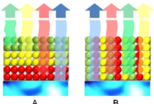
We developed our models for two basic white LED architectures. The first architecture (A) has red, yellow, and green QD layers ordered from bottom to top on the blue LED. The second architectural design (B) is the blend of red, yellow and green QDs placed on the LED (Fig. 1). Although we know that it will perform worse, we also studied the case where the

order of the QD layers in A is reversed (Arev) for the purposes of comparison. The

corresponding photon transfer equations are derived using system modeling of control theory whose details are given in the Appendix. Every box in the model corresponds to a particular process of emission or absorption with a corresponding fraction (or probability) of photons going through the associated process within or between the specified QD layers. This model assumes that there exists a metallic contact serving as a perfect mirror; as a result, all of the photons leave the device from its upper part. Since recently near-unity extraction efficiencies are achieved experimentally using special surface designs [13,14], we anticipated 100% outcoupling of the photons at the air-QD interface to reveal the ultimate potential of QD-WLEDs. Furthermore, we designed our models ignoring the scattering due to QDs. In our computations, we used two different PCEs of blue LED: one is taken with a unity PCE, which is used to understand the performance on an ideal device and identify the effects of color conversion alone, whereas the second one is taken as a state-of-the-art, high-performance LED with an experimentally demonstrated PCE of 81.3% [15].

Fig. 1. Illustration of layered (A) and blend (B) architectures.

3. Analyses and discussions

3.1 PCE and LE limits of QD-WLEDs

We start our analyses with PCE and LE for the ideal case of 100% quantum efficiency (η) of QDs. As summarized in Table 1, only as a result of the color conversion (Stoke’s shift), at least 17% of the optical power is lost as far as photometrically efficient spectra are considered

for all of the architectures. This corresponds to an LE of 315.0 lm/Welect if an ideal blue LED

is used. If a state-of-the-art blue LED having a reported PCE of 81.3% is taken into account, the maximum achievable PCE drops to 67% and the maximum achievable LE reduces to

256.1 lm/Welect. These results show that QD-WLEDs have the potential to surpass the

ultra-efficiency limitations stated for conventional LEDs in Ref. 2 if high extraction efficiencies and high PCE of blue LEDs are realized.

(5)

Table 1. Maximum, Minimum, Average and Standard Deviation of PCE (Taking Unity PCE of the Blue LED) and LE (Taking a PCE of 81.3% for the Blue LED) for the

Photometrically Efficient Spectra

max. min. aver. st. dev. PCE (%)

(with 100% PCE of blue LED) 82.7 81.6 82.1 0.3 LE (lm/Welect)

(with 81.3% PCE of blue LED) 256.1 253.2 254.3 0.8 3.2 Effects of color conversion layer architecture and quantum efficiencies on LE

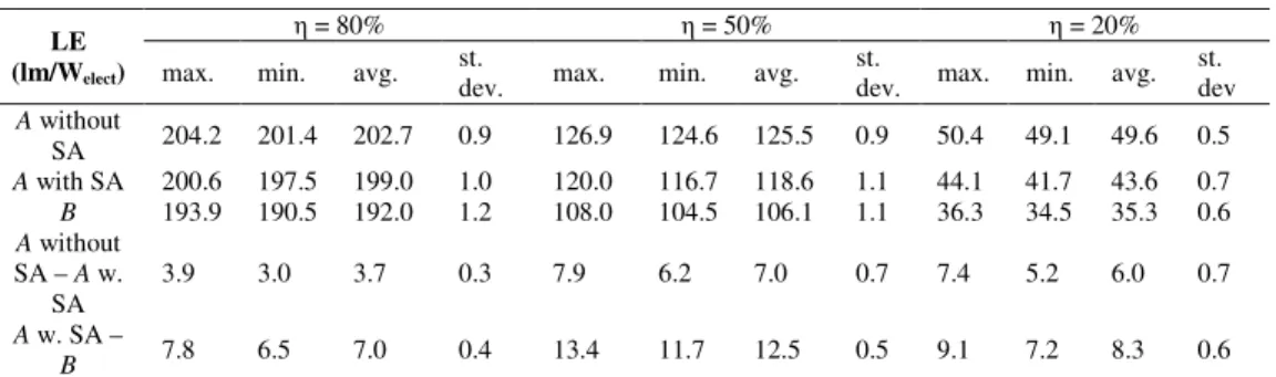
We further investigated the effect of color conversion architectures and quantum efficiencies on LE. Here we fixed the quantum efficiencies of the two QD-WLED architectures and computed their corresponding LEs and PCEs (Table 2 and 3). Our analyses showed that the layered QDs in A perform better compared to the blend QDs in B. Furthermore, LE and PCE are observed to exhibit a very narrow standard deviation for photometrically efficient spectra considered in these models. Though it is not a strong change, we observed that the self-absorption (SA) of the photons (for example, self-absorption of green photons by the green QDs) increases the standard deviation of both LE and PCE. Moreover, reversing the order of the

QD layers in A (Arev) results in a worse performance level compared to A and B.

3.3 Minimum quantum efficiencies required for achieving representative LE values

A further analysis is carried out to find the minimum η for limiting LE values (with a PCE of the blue LED taken as 81.3%) assuming the same quantum efficiencies for all of the QD layers. Our results showed that the quantum efficiencies of QDs should be at least 43% and

47% in the color conversion film for A and B, respectively, to obtain an LE of 100 lm/Welect.

In order to achieve an LE of 150 lm/Welect, η should be at least 61% and 65% in the film for A

and B, respectively. When this LE limit is increased to 200 lm/Welect, the corresponding

quantum efficiency limits become 80% and 82% in the film for A and B, respectively.

Table 2. Maximum, minimum, average and standard deviation of LE (with PCE of the blue LED taken as 81.3%) in lm/Welect for the photometrically efficient spectra with QD’s

η = 80%, 50% and 20% for two different architectures: A and B. The effect of

self-absorption (SA) is also investigated for architecture A. LE

(lm/Welect)

η = 80% η = 50% η = 20%

max. min. avg. st.

dev. max. min. avg. st.

dev. max. min. avg. st. dev A without SA 204.2 201.4 202.7 0.9 126.9 124.6 125.5 0.9 50.4 49.1 49.6 0.5 A with SA 200.6 197.5 199.0 1.0 120.0 116.7 118.6 1.1 44.1 41.7 43.6 0.7 B 193.9 190.5 192.0 1.2 108.0 104.5 106.1 1.1 36.3 34.5 35.3 0.6 A without SA – A w. SA 3.9 3.0 3.7 0.3 7.9 6.2 7.0 0.7 7.4 5.2 6.0 0.7 A w. SA – B 7.8 6.5 7.0 0.4 13.4 11.7 12.5 0.5 9.1 7.2 8.3 0.6

(6)

Table 3. Maximum, minimum, average and standard deviation of PCE (with PCE of the blue LED taken as 100%) in percentages for the photometrically efficient spectra with

QD’s η = 80%, 50% and 20% for two different architectures. The effect of self-absorption (SA) is also investigated for architecture A.

PCE (%)

η = 80% η = 50% η = 20%

max. min. avg. st.

dev. max. min. avg. st.

dev. max min. avg st. dev A without SA 64.9 63.8 64.3 0.4 42.9 37.4 39.8 0.3 17.2 14.4 15.6 0.2 A w. SA 66.0 65.0 65.5 0.4 41.1 31.9 36.0 0.4 15.6 9.7 12.4 0.3 B 62.7 61.3 62.0 0.5 37.2 30.0 32.8 0.4 12.4 9.4 10.8 0.2 A without SA – A w. SA 1.3 1.0 1.2 0.1 2.6 2.0 2.3 0.2 2.4 1.7 1.9 0.2 A w. SA – B 2.5 2.1 2.2 0.1 4.3 3.8 4.0 0.2 2.9 2.3 2.7 0.2

3.4 Photon transfer relations in architectures A and B

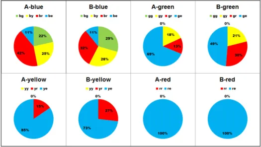
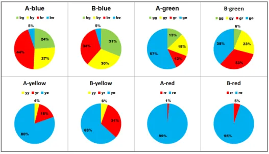
We further investigated the photon transfer in A and B at η = 100% and η = 50%. The results are presented in Fig. 2 and 3, respectively. When η = 100%, most of the blue photons are absorbed within the red layer in both of the architectures. The second most absorbing layer for blue photons is the yellow QD layer in A. For the blend case, green and yellow QDs absorb almost the same number of blue photons. As opposed to blue photons, however, most of the green photons are extracted without being absorbed. When it comes to the transfer of the yellow photons, we again observe that they are mostly extracted whereas a small amount is absorbed within the red QDs. We further find that the number of yellow photons transferred to the red QD layer is higher in B compared to A. In the case of η = 50%, photon transfer behavior does not change significantly for A and B. An important point worth mentioning for the architecture A is that still more than 50% of green photons manage to be transferred to the top despite the self-absorption.

Fig. 2. Fraction of the blue photons transferred to the green QDs (bg), to the yellow QDs (by), to the red QDs (br), and being extracted (be); fraction of the green photons self-absorbed (gg), transferred to the yellow QDs (gy), to the red QDs (gr), and being extracted (ge); fraction of the yellow photons self-absorbed (yy), transferred to the red QDs (yr), and being extracted (ye); and fraction of the red photons self-absorbed (rr) and being extracted (re) in A and B at η = 100%.

(7)

Fig. 3. Fraction of the blue photons transferred to the green QDs (bg), to the yellow QDs (by), to the red QDs (br), and being extracted (be); fraction of the green photons self-absorbed (gg), transferred to the yellow QDs (gy), to the red QDs (gr), and being extracted (ge); fraction of the yellow photons self-absorbed (yy), transferred to the red QDs (yr), and being extracted (ye); and fraction of the red photons self-absorbed (rr) and being extracted (re) in A and B at η = 50%.

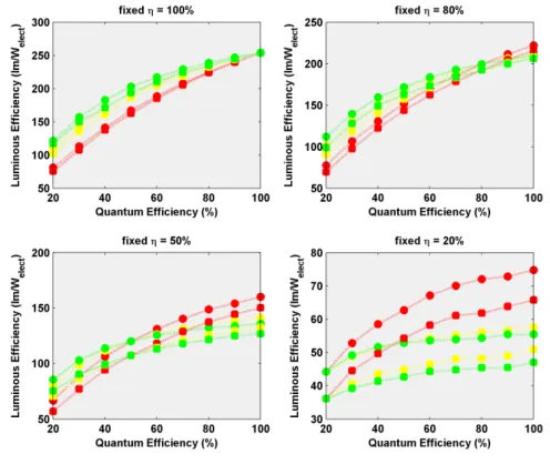
3.5 Sensitivity of PCE on the quantum efficiency change of QDs in different architectures We investigated the effect of quantum efficiency variation of QDs in different architectures. For this purpose, we fixed the efficiencies of two of the QD types and changed the efficiency of the remaining one between 20% and 100%. As test designs, spectra giving the highest PCE when three η values are equal, are selected. Corresponding results are illustrated in Fig. 4. In the case that η is fixed at 100%, the red component affects PCE and LE of the device more severely compared to other components in all architectures. When η is fixed at 80%, PCE and LE are still most sensitive to the efficiency changes of the red QDs both in A and B. Fixing η at 50% and 20% do not change the behavior stated for η = 80% case. The main reason of the criticality of the red QD efficiency is the strong amplitude of the red component in the photometrically efficient spectra [10].

(8)

Fig. 4. The luminous efficiency as a function of the variation in quantum efficiency for architectures A and B. In this analysis, ηQD of two of the QD luminophors is fixed at 100%,

80%, 50%, and 20%; ηQD of the remaining QD luminophor is changed between 20% and

100%. The points shown in the figure correspond to the luminous efficiency of QD color component whose efficiency spans this range.

3.6 Effect of quantum efficiency change on the spectral content

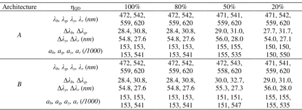
We also investigated whether the variation in the quantum efficiency affects the optimal spectral content of QD-WLEDs by calculating the average peak emission wavelength, full-width at half-maximum and weight of every color component of the spectra having PCE larger than the average PCE at that quantum efficiency. Our analyses showed that there is no significant change in the spectral content as η changes. Corresponding values can be found in Table 4.

(9)

Table 4. Average of the spectral parameters belonging to the spectra whose PCE is larger than the average PCE of the photometrically efficient spectra in A and B while varying quantum efficiencies. λi: peak emission wavelength, ∆λi: full-width at half-maximum, ai:

weight of the color component i. i is either blue (b), green (g), yellow (y) or red (r).

Architecture ηQD 100% 80% 50% 20% A λb, λg, λy, λr (nm) 472, 542, 559, 620 472, 542, 559, 620 471, 541, 559, 620 471, 542, 559, 620 ∆λb, ∆λg, ∆λy, ∆λr (nm) 28.4, 30.8, 54.8, 27.6 28.4, 30.8, 54.8, 27.6 29.0, 31.0, 56.0, 28.0 27.7, 31.7, 54.0, 27.1 ab, ag, ay, ar (/1000) 153, 153, 153, 541 153, 153, 153, 541 155, 155, 155, 535 150, 150, 150, 550 B λb, λg, λy, λr (nm) 472, 542, _{559, 620} 472, 542, _{559, 620} 472, 543, _{558, 620} 471, 541, _{559, 620} ∆λb, ∆λg, ∆λy, ∆λr (nm) 28.4, 30.8, 54.8, 27.6 28.4, 30.8, 54.8, 27.6 30.0, 32.7, 55.3, 27.3 29.0, 31.0, 56.0, 28.0 ab, ag, ay, ar (/1000) 153, 153, 153, 541 153, 153, 153, 541 151, 151, 151, 547 155, 155, 155, 535 4. Conclusion

In this work we developed models to study the power conversion efficiency and luminous efficiency of QD-WLEDs. Using these models we investigated the effect of quantum efficiency variation on PCE and LE. Furthermore, we found that QD-WLEDs can be both photometrically and electrically more efficient than phosphor based white LEDs when QDs and LEDs with high efficiencies are jointly used. When we consider one of the best blue LEDs having a PCE of 81.3%, PCE of the white light emitting device is 67.0% and LE is

256.1 lm/Welect, while high photometric performance is achieved, i.e., with the color rendering

index ≥90 (with the rendering index of the test color 9 at least 70), the luminous efficacy of

optical radiation ≥380 lm/Wopt, the correlated color temperature ≤4000 K and the chromaticity

difference dC <0.0054. The highest obtainable PCE of the QD-WLED is 82.7% if PCE of the blue LED chip is unity. In addition to these, we also found that placing red, yellow and green QD layers in order on blue LED (architecture A) is the most efficient one for color conversion

QD-WLEDs compared to the QDs having the reversed order (architecture Arev) and QD

blends (architecture B). By employing the architecture A and a blue LED chip having a PCE of 81.3%, one needs to use QDs with 43%, 61% and 80% quantum efficiencies to reach the

luminous efficiencies of 100, 150 and 200 lm/Welect, respectively. The change in the

efficiencies of the red QDs leads to a stronger effect on PCE and LE of the device when the quantum efficiencies of the other quantum dots are fixed at 100%, 80%, 50% and 20%. We found out that the main reason for this behavior is the higher red content in the spectra having high photometric performance.

5. Appendix

To increase the readability of this letter, we explain the details of our calculation methodology in this separate section. The readers, who do not want to pay attention in these details, may ignore this part.

In addition to the assumptions stated in the second section, the spectral emission profile of blue LED and QDs are taken to be Gaussian, which matches experimentally well. We further assumed that all of the photons within the same Gaussian spectrum experience the same absorption coefficient; since these QDs have narrow and symmetric emission bands, most of the absorption occurs around the peak of the Gaussian, which can be characterized by a single absorption constant. This assumption provides very good approximations when the peak wavelength of the Gaussian spectrum to be absorbed is far away from the excitonic peak of the absorbing QD layer. The largest error occurs when the peak of the emission spectrum is in the proximity of the excitonic peak of the absorbing QD layer. For the QD film thicknesses we are using, however, this causes a maximum error of ca. 0.1 in the absorbed photon

(10)

fraction. Therefore, self-absorption (SA) is underestimated. As the quantum efficiencies decrease, the corresponding layer thicknesses increase. As a result, this deviation from the correct value is observed to diminish. Another assumption is that a fraction k of the generated photons from QDs is emitted upwards, and remaining 1-k fraction is emitted downwards. The results we present correspond to the case of k = 1/2, which is typically the case for almost spherical QDs used here.

To calculate PCE and LE, the first step is to relate the emission spectrum of QDs to their absorption spectrum. For this purpose, commonly used spherical CdSe QDs are chosen because of the availability of the required information in the literature. Fitting a linear curve

to the data provided by Boatman et al. [16], the emission peak (λem) and the first exciton peak

of the absorption spectrum (λabs) are related as in Eq. (3):

8.3045 1.0308 em abs λ λ = − (3)

The absorption spectrum of QD films are obtained from Ref. 17 and absorbed fraction is converted to absorption coefficient for large QDs having a thickness of 200 nm. The absorption coefficient of a QD is then found by using the data obtained from Ref. 16 in

accordance with its λabs.

The power conversion efficiency of a QD-WLED based on color conversion principle can

be calculated when the necessary number of blue photons (Sb1) pumping QDs is computed

given the number of photons (per unit time) in all of the color components in the final white light spectrum, i.e., blue (Sb), green (Sg), yellow (Sy) and red (Sr). The calculation of Sb1,

which will be explained later in detail, is dependent on the architecture. To find the power conversion efficiency of the simulated white LED, the number of the photons coming out of

the blue LED (Sb1) should be compared to a state-of-the-art blue LED [15], which has a power

conversion efficiency (PCE) of 81.3%. Given an input electrical power (Pelect,LED) of 1 W, this

LED will deliver an optical power (Popt,LED) of 813 mW. We relate the optical power of the

blue LED to the number of its blue photons as in Eq. (4):

, 1 ( , , )

opt LED b LED b b

P =γ

∫

S g λ λ ∆λ dλ (4)

where gLED(λ,λb,∆λb) is the spectral power distribution of the blue LED modeled as a

normalized Gaussian function centered at its peak emission wavelength (λb) with a given

full-width-at-half maximum (∆λb), which is normalized to have a total of one photon under its

Gaussian curve. Thus, the proportionality factor γ is given in Eq. (5): , 1 ( , , ) opt LED b LED b b P S g d γ λ λ λ λ = ∆

∫

(5)

As a result, the number of photons for the color components scaled with respect to the real LED is given by Eq. (6)–(9):

, b final b S =γS (6) , y final g S =γS (7) , r final y S =γS (8) , r final r S =γS (9)

Using the spectral power distribution g(λ,λi,∆λi) for each color component i (i = b, g, y, r),

each modeled as a normalized Gaussian function centered at the wavelength λi having a

full-width-at-half-maximum of ∆λi with a unity number of photons in color i, the resulting spectral

(11)

( )

(

)

₍

₎

(

)

(

)

, , , , , , ∆ , ∆ , ∆ , ∆ , , , b final b b g final g g y final y y r final r r s S g S g S g S g λ λ λ λ λ λ λ λ λ λ λ λ = + + + λ (10)

Resultantly, the power conversion efficiency (PCE) is given by Eq. (11).

( )

elect s d PCE P λ λ =

∫

(11)

Finally, the luminous efficiency (LE) is equivalent to the product of power conversion efficiency and the luminous efficacy of optical radiation (LER), as given by Eq. (12):

LE=PCE LER× (12)

5.1 Computational modeling of architectures

In this work, we have calculated PCEs of two basic architectures of QD-WLEDs. The first architecture consists of red, yellow, and green QD layers placed in order from bottom to top on a blue LED chip (A). The second one models the film made of the blend of these QDs. Moreover, we modeled a third architecture by reversing the order of QD layers in A, which is

denoted as Arev, to compare with the original architecture (A) and the second basic one (B).

However, it was obvious from the beginning that this structure will perform worse as a consequence of increasing photon transfer to subsequent QD layers due to the order of QD layers.

5.1.1 Modeling architecture A

In A (and Arev) c1, c2 and c3 denote the fraction of blue photons absorbed by green, yellow and

red QDs, respectively. c4 and c5 denote the fraction of green photons absorbed by yellow and

red QDs, respectively, whereas absorbed fraction of yellow photons within the red layer is

expressed as c6. By using the approximations stated in the previous section, we can relate c4,

c5 and c6 to c2 and c3 as in Eq. (13) and (14).

4 2 ( ) 1 (1 ) ( ) y g y b c c α λ α λ ≈ − − (13) 5 3 ( ) 1 (1 ) ( ) r g r b c c α λ α λ ≈ − − (14) 6 3 ( ) 1 (1 ) ( ) r y r b c c α λ α λ ≈ − − (15)

where αi(λj) stands for the absorption coefficient of QD layer of color i at the peak emission

wavelength of Gaussian function emitting in color j. It is observed that this assumption does not yield an important deviation from the exact value; additionally, it provides simplicity in calculations and speed in numerical solutions of the equations by avoiding dealing with

broadband spectra. Since we have four equations that include our known parameters (i.e., Sb,

Sg, Sy and Sr), we have enough information to find Sb1, c1, c2 and c3. As we find Sb1, we can

calculate PCE of the QD-WLED in architecture A.

The self-absorption (SA) fractions are also included in the calculations; however, their mathematical formulation is not as simple as the previous ones. In addition, this depends on the architecture, type of absorbing QDs, wavelength of the absorbed photons and the pathway of the generated photon (for example, yellow photons generated due to the absorption of blue and green photons have different photon self-absorption fractions). In all of the architectures,

(12)

denotes the self-absorbed fraction of photons when propagating downwards. Additionally, c”b

is used to express the fraction of self-absorbed photons while propagating upwards after the reflection of downwards emitted photons. When referring to a single photon, all these aforementioned fractions actually correspond to probabilities.

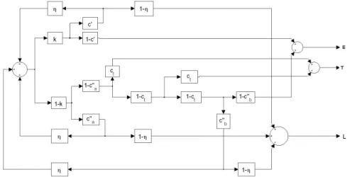
In A upon absorption of a photon by a QD layer, a new photon is generated and emitted upwards with a probability of k (1/2 in the case of an isotropic QD) and downwards with a probability of 1-k (1/2 for the isotropic QD). Upwards emitted photons are self-absorbed by the same QD layer with a probability of c’. These photons might be reemitted with a probability of η and lost with a probability of 1-η due to non-radiative recombination.

Downwards emitted photons are absorbed within the same QD layer with a probability of ca”,

these photons are reemitted with a probability of η and lost with a probability of 1-η. Photons

survived from SA might transfer their energies to other QD layers with a probability of ct.

When the survived ones are reflected back, there is again a probability of ct to be absorbed by

other QD layers. The remaining photons have a probability of cb” being absorbed within the

same layer that they are emitted. These absorbed photons are reemitted and lost with probabilities of η and 1-η, respectively. Finally, photons survived from SA are extracted with

a probability of 1-cb”. These photon transfer processes are illustrated in Fig. 5.

Fig. 5. Illustration of optical mechanisms using system box model for architecture A.

Solution of these transfer functions results in the probabilities of extraction (E), transfer to other QD layers (T) and loss due to SA (L). Corresponding equations are given in Eq. (16)– (18). ' " 2 " ' " " 2 " (1 ) (1 )(1 )(1 ) (1 ) 1 (1 ) (1 )(1 )(1 ) a t b a a t b k c k c c c E kcη k c η k c c c η − + − − − − = − − − − − − − (16) " ' " " 2 " (1 )(1 ) [1 (1 )] 1 (1 ) (1 )(1 )(1 ) a t t a a t b k c c c T kcη k c η k c c c η − − + − = − − − − − − − (17) ' " 2 " " ' " " 2 " (1 )[ (1 )(1 )(1 ) (1 ) ] 1 (1 ) (1 )(1 )(1 ) a t b a a a t b kc k c c c k c L kc k c k c c c η η η η − + − − − + − = − − − − − − − (18)

SA probabilities for photons in a QD layer having color m with an excitation path of j are given in Eq. (19)–(21).The bottom of QD layers corresponds to z = 0, and its film thickness is zm.

(13)

( )

( )( ) 0 '' (1 ) m m m m z z z mja mj c =

∫

d z −e−α λ − dz (19)

( )

( ) '' 0 (1 ) m m m z z mja mj c =

∫

d z −e−α λ dz (20) ( ) '' 1 m mzm mjb c = −e−α λ (21)

where dmj(z) denotes the normalized excitation profile and correspondingly generated photon

distribution due to this excitation within the QD layer. The normalization is carried out such

that its integral between z = 0 and z = zm is unity. Green, yellow and red photons generated by

the excitation of blue photons have a distribution of dg0(z), dy0(z) and dr0(z) within green,

yellow and red layers, respectively. Yellow and red photons generated by the excitation of

green photons have a distribution of dyg(z) and drg(z) within yellow and red QD layers,

respectively. The distribution of blue photons within green, yellow and red QD layers are

given in Eq. (22), where m stands for green (g), yellow (y) or red (r) QDs. κm0 is the

normalization coefficient and λb is the peak emission wavelength of blue LED. Since blue

photons pump QDs from bottom, they experience an exponential decay. As a result, QDs excited by blue LED should generate photons with the same distribution. Therefore, Eq. (22) actually formulates the normalized distribution of photons of color m generated by the excitation of blue photons within the QDs emitting in color m.

( )

0( ) 0

m b z

m m

d z =κ e−α λ (22)

The distribution of the green photons within the yellow layer is given in Eq. (23). κyg is the

normalization coefficient, zy is the thickness of the yellow QD layer, λg is the peak emission

wavelength of the green QDs and αy is the absorption spectrum of the yellow QDs. The first

summand in Eq. (23) is the distribution of downwards propagating photons, whereas the second one is due to the SA after reflection from the bottom mirror.

( )

( )( )

(

)(

)

( ) ( )( )

(

)(

)

( ) y g y y g y g y y g α λ z z 2 α λ z α λ z z 4 5 yg 2 α λ z 4 5 [e 1 c 1 c e ]e κ 1 c 1 c e yg d z − − − − − − + − − = _ _   + − −  (23)

The green photons are distributed within the red layer as given in Eq. (24). κrg is the

normalization coefficient, zr is the thickness of the red QD layer, λg is the peak emission

wavelength of the green QDs and αr is the absorption spectrum of the red QDs. Similar to the

distribution of green photons within the yellow QDs, the first summand in Eq. (24) stands for the absorption of downward emitted photons and the second one corresponds to their self-absorption (SA) within the red QDs after being reflected from the bottom mirror.

( )

{

αr( )λg(zr z) αr( )λgz α λr( )g(zr z) αr( )λg z

}

rg 5 5

κ [e (1 c )e ]e (1 c )e

rg

d z = − − + − − − − + − − (24)

Finally, the distribution of the yellow photons within the red layer is given in Eq. (25).

The same conventions are used, κry stands for the normalization coefficient, zr is the thickness

of the red QD layer, λy and αr denote the peak emission wavelength of the yellow QDs and the

absorption spectrum of the red QDs, respectively. The first and second summands of Eq. (25) express the same absorption mechanisms as in Eq. (24), but this time yellow photons are absorbed instead of green photons.

( )

{

αr( )λy(zr z) αr( )λyz αr( )λy(zr z) α λr( )yz

}

ry 6 6

κ [e (1 c )e ]e (1 c )e

ry

d z = − − + − − − − + − − (25)

The photon transfer probabilities for green, yellow and red photons are formulated by Eq. (26)–(28). Equation (26) denotes the absorption probability of green photons by the yellow

(14)

and red QD layers and Eq. (27) is the formulation for the probability of yellow photons to be absorbed by the red QD layer.

2 4 (1 4)(1 5) 4 (1 4) 5 (1 4)(1 5) 5 tg c =c + −c −c c + −c c + −c −c c (26) 6 6(1 6) ty c =c +c −c (27) 0 tr c = (28)

If the number of blue photons emitted from the blue LED is Sb1, then the number of

generated green photons (Sg0) can be found using Eq. (29) and the number of extracted

photons (Sgn) is given by Eq. (30). Similarly, the number of yellow photons generated by blue

(Sy0) and green (Syg0) photons can be calculated using Eq. (31) and (32), respectively. The

number of extracted yellow photons is given by Eq. (33). The number of red photons

generated by blue photons (Sr0) is given by Eq. (34), the number of red photons generated by

green photons (Srg0) is given in Eq. (35), the number of red photons generated by yellow

photons, which are generated through pumping of the yellow QDs by blue (Sry0) and green

(Sryg0) photons, is found using Eq. (36) and Eq. (37), respectively. Finally, the number of

extracted red and blue photons (Srn and Sbn) are calculated using Eq. (38) and (39),

respectively. 0 1 1(1 2)(1 3) g b g s =s c −c −c η (29) 0 0 gn g g s =s E (30) 0 1(1 3) 2 y b y s =s −c cη (31) 2 4 4 5 4 0 0 0 2 4 4 5 4 5 4 5 4 5 (1 )(1 ) (1 )(1 ) (1 ) (1 )(1 ) yg g g y c c c c s s T c c c c c c c c c η + − − = + − − + − + − − (32) 0 0 0 yn y y yg yg s =s E +s E (33) 0 1 3) r b r s =s c η (34) 5 4 5 4 5 0 0 0 2 4 4 5 4 5 4 5 4 5 (1 ) (1 )(1 ) (1 )(1 ) (1 ) (1 )(1 ) rg g g y c c c c c s s T c c c c c c c c c η + − + − − = + − − + − + − − (35) 0 0 ry y yg r s =s T η (36) 0 0 ryg yg yg r s =s T η (37) 0 0 0 0 0 rn r r rg rg ry ry ryg ry s =s E +s E +s E +s E (38) 1(1 1)(1 2)(1 3) bn b s =s −c −c −c (39)

Since Sbn, Sgn, Syn and Srn are known parameters, Sb1 can be found using Eq. (30), (33), (38)

and (39); as a result, PCE of the QD-WLED having the architecture A can be calculated.

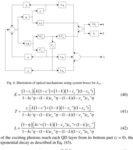
5.1.2 Modeling architecture Arev

When the order of QDs is reversed, main optical mechanisms do not change; therefore, the mathematical notation does not change significantly. The only difference between

architectures A and Arev occurs in the probability of photons transferred to other QD layers. In

A, photons are transferred only during downward emission (and after reflection from the

bottom mirror). If the QD order is reversed, photons can transfer their energies to other QD layers only while propagating upwards. Corresponding optical mechanisms are illustrated in

'' 1 ' (1 ) '' (1 )(1 '') '' a b a a a b kc k c c k c L kc k c k c c η η η η − _ + − − + − _ = − − − − − − (42)

Because all of the exciting photons reach each QD layer from its bottom part (z = 0), they experience an exponential decay as described in Eq. (43).

( )

( ) m j z

mj mj

d z =κ e−α λ (43)

where κmj is the normalization constant over the integral from z = 0 to z = zm. Furthermore, the

transfer probability of green photons to other QD layers is c4 + (1-c4)c5, and the transfer

probability of yellow photons to the red QD layer is c6. Finally, the transfer probability for red

photons to another layer is taken as zero.

If the number of blue photons emitted from the blue LED is given as Sb1, the number of

generated green photons (Sg0) is given by Eq. (44) and the number of extracted green photons

(Sgn) by Eq. (45). Similarly, the number of yellow photons generated by blue (Sy0) and green

(Syg0) photons is expressed by Eq. (46) and (47), respectively. The number of yellow photons

being extracted is given in Eq. (48). The number of red photons generated by blue photons

(Sr0) is given in Eq. (49), the number of red photons generated by green photons (Srg0) is

expressed by Eq. (50), the number of red photons generated by yellow photons, which are

generated through pumping of yellow QDs by blue (Sry0) and green (Sryg0) photons, is

formulated by Eq. (51) and Eq. (52), respectively. Finally, the number of red and blue photons

being extracted (Srn and Sbn) are given in Eq. (53) and (54), respectively.

0 1 1

g b g

(16)

0 0 gn g g S =S E (45) 0 1(1 1) 2 y b y S =S −c cη (46) 4 0 0 0 4 (1 4) 5 yg g g y c S S T c c c η = + − (47) 0 0 0 yn y y yg yg S =S E +S E (48) 0 1(1 1)(1 2) 3 r b r S =S −c −c cη (49) 5 4 0 0 0 4 4 5 (1 ) (1 ) rg g g r c c S S T c c c η − = + − (50) 0 0 ry y yo r S =S T η (51) 0 0 ryg yg yg r S =S T η (52) 0 0 0 0 0 rn r r rg rg ry ry ryg ry S =S E +S E +S E +S E (53) 1(1 1)(1 2)(1 3) bn b S =S −c −c −c (54)

Since Sbn, Sgn, Syn and Srn are known, solutions of Eq. (45), (48), (53) and (54) give us Sb1

and the PCE of the simulated QD-WLED in case that the color converting quantum efficiencies of QDs are available.

5.1.3 Modeling architecture B

The absorption and emission within a film of QD-blend are different than the previous ones. In the previous architectures, photon energy transfer to other layers occurs either during upward or downward emissions because of the order of QD layers. In blends, however, photon absorption occurs during both emission directions. Thus, we changed our notation regarding photon transfer by separating photon transfer probabilities to other type of QDs for upward and downward emission. We modeled the blend structure as infinitesimally thin QD columns as illustrated in Fig. 1. All of these QD columns have the same thickness in

z-direction, zl, and the fractional QD densities are introduced to our equations so that the green

QD fraction (fg), yellow QD fraction (fy) and red QD fraction (fr) sum up to unity. Then, a

photon with high energy excites the QDs with a probability scaled by the QD-fraction (f); therefore, photon transfer probabilities (or fractions) should be scaled accordingly.

The photon transfer mechanisms are illustrated in Fig. 7 using the system box approach. In

addition to the notation used in the previous model, cta” denotes the photon energy transfer

probability to other QD layers during downward propagation and ctb” denotes the photon

energy transfer probability of downward emitted photons to other QD layers after being reflected from the bottom mirror. The probabilities of photons being extracted (E), those being transferred to other QDs (T) and those being lost (L) due to SA are given in Eq. (55)– (57). The self-absorption probabilities are given by Eq. (58)–(60) for upward and downward emission (before and after reflection), respectively.

(17)

Fig. 7. Illustration of optical mechanisms using system boxes for B.

(

)

(

)(

)

(

)

(

)

1 ' (1 ' ) 1 1 '' (1 '')(1 )(1 ) 1 [ ' 1 (1 ) 1 (1 ) ] '' '' '' '' '' '' t a ta b tb a a ta b k c c k c c c c E kc k c k c c c η − − + − − − − − = − + − + − − − (55)

(

)

(

)

(

)

(

)

(

)

'' '' ' 1 ' ' 1 (1 ) 1 (1 ')( '' '' '' ' '' '' '' '' 1 )(1 ) 1 [ 1 (1 ) 1 (1 ) ] t a ta a ta b tb a a ta b k c c k c c k c c c c T kc k c k c c c η − + − − + − − − − = − + − + − − − (56)

(

)

(

)

(

)

(

)

'' '' '' '' (1 )[ ' 1 (1 )(1 ) 1 ] 1 [ ' 1 '' (1 ) 1 '' (1 '') ' ]' a ta b a a a ta b kc k c c c k c L kc k c k c c c η η − + − − − + − = − + − + − − − (57)

( )

( )(1 ) 0 (1 ) l m m z z z mj m m c′ =

∫

f d z −e−α λ − dz (58)

( )

( ) '' 0 (1 ) l m m z z mja m mj c =

∫

f d z −e−α λ dz (59) ( ) '' (1 m mzl) mjb m c = f −e−α λ (60)

where dmj(z) denotes the normalized distribution of photons over the integral from 0 to zl. m

stands for the color of the QDs: g for green, y for yellow and r for red QDs. j stands for the path of excitation. The same nomenclature is followed as for m. In addition, here 0 means the excitation coming from the pump LED. For example, the red QDs excited by yellow photons, which are generated through absorption of first blue photons in the green QDs and then through the absorption of green photons in the yellow QDs, are abbreviated as yg0. Then

self-absorption probability of upward emission for this special case becomes c’ryg0. Similarly,

green, yellow and red QDs excited by blue photons have a distribution of blue photons dg0(z),

dy0(z) and dr0(z) within green, yellow and red layers, respectively. Yellow and red QDs

excited by green photons have distribution functions of green photons within yellow and red

QD layers of dyg0(z) and drg0(z), respectively. Finally, the distribution of yellow photons

within the red QDs are dryg0(z) and dry0(z) depending on the excitation path. The first one

stands for the yellow photon distribution within the red QDs when yellow photons are generated by the wavelength up-conversion of green photons in the yellow QDs. The latter one denotes the yellow photon distribution within the red QDs when yellow photons are generated by the wavelength up-conversion of blue photons in the yellow QDs.

(18)

The normalized distribution of blue photons within green (g), yellow (y) and red (r) QDs

is as given in Eq. (61), where m is g, y or r, respectively, κm0 is the corresponding

normalization coefficient over the integral between z = 0 and z = zl. Furthermore, λb is the

peak emission wavelength of blue LED.

( )

0( ) 0

m b z

m m

d z =κ e−α λ (61)

The normalized distribution functions of green photons within the yellow QDs are given

by Eq. (62) where κyg0 is the normalization constant. This depends on the distribution of green

photons. Additionally, it contains the distribution of green photons in the yellow QDs while propagating upwards and downwards, denoted in the first and second summands of Eq. (62), respectively. Furthermore, it includes terms for the distribution of green photons within the yellow QDs, which are not absorbed by the green, yellow and red QDs during downward emission but absorbed in the yellow QDs after the reflection from the bottom mirror, as expressed in the third, fourth and fifth summands of Eq. (62), respectively.

( )( ) ( )( ) 0 0 ( ) ( ) 0 0 0 0 ( ) ( ) ( ) ( ) 0 0 ( ) ( ) l l y g i y g i l y g g g i l l y g y g i y g r g i z z z z z z y i y i z z z yg yg g y g i z z z z z z y y i y r i f e dz f e dz d z k d z f e f e dz f e f e dz f e f e dz α λ α λ α λ α λ α λ α λ α λ α λ − − − − − − − − − −   + +         = +       +    

∫

(62)

The normalized distribution of green photons within the red QDs is very similar to the

previous case and given in Eq. (63), where κrg0 is the normalization constant. As in the

previous equation, this distribution depends on the distribution of green photons. Furthermore, it contains the distribution of green photons absorbed in the red QDs while propagating upwards and downwards, expressed in the first and second summands of Eq. (63), respectively. In addition, the distribution of green photons within the red QDs, which are not absorbed by the green, yellow and red QDs during downward emission but absorbed in the red QDs after reflection from the bottom of the device are expressed in the third, fourth and fifth summands of Eq. (63).

( )( ) ( )( ) 0 0 ( ) ( ) ( ) ( ) 0 0 0 0 0 ( ) ( ) 0 ( ) ( ) l l r g i r g i l l r g g g i r g y g i l r g r g i z z z z z z r i r i z z z z z z rg rg g r g i r y i z z z r r i f e dz f e dz d z k d z f e f e dz f e f e dz f e f e dz α λ α λ α λ α λ α λ α λ α λ α λ − − − − − − − − − −   + +         = + +          

∫

(63)

The distribution of yellow photons, which are generated through the pumping of blue

photons, within the red QDs has also a similar behavior, given by Eq. (64). Again κry0 is the

normalization constant, and the distribution is scaled with dy0(z). This depends also on the

distribution of yellow photons absorbed in the red QDs while propagating upwards and downwards, as the first and second summands of Eq. (64) present, respectively. In addition, the distribution function of yellow photons within the red QDs, which are not absorbed by the yellow or red QDs during downward emission but absorbed in the red QDs after reflection from the bottom of the device, are expressed in the third and fourth summands of Eq. (64).

(19)

( )( ) ( )( ) 0 0 ( ) ( ) ( ) ( ) 0 0 0 0 0 ( ) ( ) l l r y i r y i l l r y y y i r y r y i z z z z z z r i r i z z z z z z ry ry y r y i r r i f e dz f e dz d z k d z f e f e dz f e f e dz α λ α λ α λ α λ α λ α λ − − − − − − − −   + +         = + +          

∫

(64)

The distribution of yellow photons, which are generated through the excitation of green photons, within the red QDs is almost identical to Eq. (65). In this case, the distribution is

scaled by dyg0(z) instead of dg0(z) and a new normalization coefficient, κryg0, is required. The

final form of the expression is given in Eq. (65).

( )( ) ( )( ) 0 0 ( ) ( ) ( ) ( ) 0 0 0 0 0 ( ) ( ) l l r y i r y i l l r y y y i r y r y i z z z z z z r i r i z z z z z z ryg ryg yg r y i r r i f e dz f e dz d z k d z f e f e dz f e f e dz α λ α λ α λ α λ α λ α λ − − − − − − − −   + +         = + +          

∫

(65)

The photons emitted by the green QDs can be transferred to yellow and green QDs. These transfer probabilities for upward emission, downward emission before and after the reflection from the bottom of the device are given in Eq. (66)–(68), respectively.

( ) ( )( ) ' 0 0 0 0 0 ( ) (1 ) ( ) (1 ) l l y g r g l z z z z z tg g y g r c =

∫

d z f −e−α λ dz+

∫

d z f −e−α λ − dz (66) ( ) ( ) " 0 0 0 0 0 ( ) (1 ) ( ) (1 ) l l y g r g z z z z tg a g y g r c =

∫

d z f −e−α λ dz+

∫

d z f −e−α λ dz (67) ( ) ( ) " 0 (1 ) (1 ) y g zl r yzl tg b r y c = f −e−α λ +f −e−α λ (68)

The photons emitted by the yellow QDs can be transferred to red QDs. These probabilities for upward emission, downward emission before and after the reflection from the bottom of the device are given for yellow QDs pumped by blue photons in Eq. (69)-(71) and for yellow QDs pumped by green photons in Eq. (72)-(74), respectively. Finally, it should be noted that all the transfer probabilities of red photons are zero.

( )

( )( ) 0 0 0 ' (1 ) l r y l z z z tyg yg r c =

∫

d z f −e−α λ − dz (69)

d z f −e−α λ dz (73) ( )

(

)

'' 0 1 r yzl tyg b r c = f −e−α λ (74)

Before stating the equations of final photon numbers, finding the ratio of green photons being transferred to the yellow (ty) and red (tr) QDs to the total fraction of green photons

transferred will make equations easier to follow. Those expressions are given in Eq. (75) and (76), respectively.

(

)

(

)

(

)

(

)

(

)(

)

(

)

(

)

(

)

(

)

(

)(

)

' ' '' '' '' '' '' '' ' ' ' '' '' '' '' '' '' '' '' 1 1 1 1 1 1 1 1 ( ) 1 1 ( ) 1 1 1 1 ( ) y a y a ta b yb y y r a y r a ta b yb rb k c c k c c k c c c c t k c c c k c c c k c c c c c − + − − + − − − − = − + + − − + + − − − − + (75) 1 r y t = − t (76)

where cy’ and cr’ are the absorption probability of green photons by the yellow and red QDs

during upward emission, respectively. cy” and cr” are the probabilities of photon transfer to the

yellow and red QDs during downward emission before getting reflected from the bottom of the device, respectively. The probabilities for both type of QDs after the reflection become

d z f −e−α λ dz (81) ( ) '' (1 r g zl) rb y c = f −e−α λ (82)

The number of generated green, yellow and red photons (Sg0, Sy0, Sr0) by blue photons are

given in Eq. (83)–(85) and the number of extracted green photons (Sgn) is given in Eq. (86).

Then, the number of extracted yellow and red photons generated by green photons (Syg0 and

Srg0), can be found using Eq. (87) and (88), respectively. The number of extracted yellow

photons (Syn) is calculated using Eq. (89). Furthermore, the number of red photons generated

by yellow photons, which are generated through excitation of the yellow QDs by blue (Sry0)

and green (Sryg0) photons, are given in Eq. (90) and Eq. (91), respectively. Finally the number

of extracted red and blue photons (Srn and Sbn) are given in Eq. (92) and (93), respectively.

( )

(

)

0 1 1 b l g z g b g g S =S f −e−α λ η (83) ( )

(

)

0 1 1 b l y z y b y y S =S f −e−α λ η (84)

(21)

( )

(

)

0 1 1 b l r z r b r r S =S f −e−α λ η (85) 0 0 gn g g S =S E (86) 0 0 0 g y yg y g S =η S T t (87) 0 0 0 g r rg r g S =ηS T t (88) 0 0 0 0 yn y y yg yg S =S E +S E (89) 0 0 0 ry y y r S =S T η (90) 0 0 0 ryg yg yg r S =S T η (91) 0 0 0 0 0 0 0 0 rn r r rg rg ry ry ryg ryg S =S E +S E +S E +S E (92) ( ) ( ) ( ) 1 g b zl y b zl r b zl bn b g y r S =S _f e−α λ + f e−α λ + f e−α λ _ (93)

Since Sbn, Sgn, Syn and Srn are known parameters, by solving Eq. (86), (89), (92) and (93)

for Sb1, power conversion efficiency of the QD-WLED can be calculated given the quantum

efficiencies of QDs (η).

Acknowledgments

We acknowledge the financial support in part by ESF EURYI, EU FP7 Nanophotonics4Energy NoE, and TUBITAK under the Project No. EEEAG 109E002, 109E004, 110E010, and 110E217, and in part by NRF-CRP6-2010-02 and NRF RF 2009-09. HVD acknowledges additional support from TUBA-GEBIP and TE acknowledges TUBITAK-BIDEB.