Metaheuristics-based pre-design guide for cantilever retaining walls

Metaheuristics-based Pre-Design Guide for Cantilever

Retaining Walls

A pre-design guide for cantilever retaining walls and a detail parametric study of such walls is presented here. Mathematical models based on statistical methods were improved for calculating safety factors of sliding, overturning, and slope stability of those walls. The harmony search algorithm (HSA)-a metaheuristic method-was employed to realize reasonable results of the pre-design guide from all distinct cases. Through the design algorithm, the optimal design was determined for varied soil types differently from suggestions of design codes. Thus, an optimal pre-design guide for safe and economic wall design was realized in a shorter time compared to the conventional method.

Keywords: Cantilever retaining wall, mathematical model, pre-design guide, external stability of the wall.

1. INTRODUCTION

In geotechnical engineering, the stability of two different soil levels is achieved by using retaining walls. In the absence of sufficient excavation areas at construction sites or docks, retaining walls act as a vertical connector, thus providing resistance to lateral soil forces. Retaining wall design must satisfy external stability conditions and be economical. In traditional retaining wall design, wall dimensions to ensure stability are determined by a trial

Note:

- This paper has been received on May 9, 2019 and accepted for publication by the Editorial Board on March 2, 2020.

- Discussions on this paper will be accepted by xxxxxxx xx, xxxx.  https://doi.org/10.18400/tekderg.561956

1 KTO Karatay University, Department of Civil Engineering, Konya, Turkey - esra.uray@karatay.edu.tr https://orcid.org/0000-0002-1121-2880

2 Konya Technical University, Department of Civil Engineering, Konya, Turkey - ozcantan@selcuk.edu.tr https://orcid.org/0000-0002-8217-1502

3 Karamanoglu Mehmetbey University, Department. of Civil Engineering, Karaman, Turkey - scarbas@kmu.edu.tr - https://orcid.org/0000-0002-3612-0640

4 Konya Technical University, Department of Civil Engineering, Konya, Turkey - iherkan@ktun.edu.tr https://orcid.org/0000-0003-4514-4553

and error method [1]. In this method, the designer may select wall dimensions randomly until the stability of the wall is satisfied. Therefore, obtaining a safe design for selected wall dimensions is time-intensive when a large number of trials is required. Furthermore, obtained wall dimensions may not be economic among all possibilities. To consider all phenomena involved in the design, using a pre-design guide in the design of the cantilever retaining wall (CRW) becomes important for the designer.

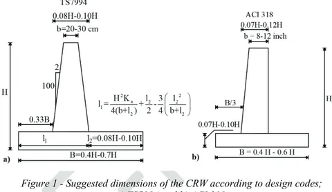
The suggested wall dimensions according to TS 7994 and ACI 318 which are implemented in the CRW design have been demonstrated in Figure 1 [2-4]. The LRFD Bridge Design Manual [5] provides the pre-design dimensions of the base length, base thickness, and toe extension. The base length should be 60%–70% of the stem height and the base thickness should be 10%–15% of the stem height. The toe extension should be ~30% of the base length.

Figure 1 - Suggested dimensions of the CRW according to design codes; a) TS7994 and b) ACI 318.

Because retaining wall design is one of the complex design problems in the field of geotechnical engineering, there is a need for new design techniques. Metaheuristic optimization algorithms, which have received considerable attention in recent years, have been effectively used for solving complex optimization problems over the last two decades [6]. Their popularity is attributed to their simplicity, compatibility to a wide range of situations, and effectiveness. Among these algorithms, harmony search algorithm (HSA) was used as an optimization tool in this study. The HSA is based on the improvisation of identifying the best harmony in any piece of music; it is more advantageous than the other metaheuristics algorithms because it is easy to use, yields result in a reasonable time even with numerous iterations, utilizes both discrete and continuous variables, and reaches the global optimal without getting trapped in local optimum solutions during optimization. Moreover, many successful applications of HSA have been used, especially in the fields of structural optimization [7], hydraulics [8], vehicle routing [9], and geotechnical engineering [10]. Furthermore, to boost the accuracy and increase the rate of convergence of the standard HSA, some modified, improved, and hybrid versions of the algorithm are specifically

proposed for determining the critical sliding surface for slopes [11], optimal foundation design [12], and optimizing reinforced cantilever retaining walls [13, 14].

Parameters such as the total wall height, the angle of internal friction, and the unit volume weight play an important role in such designs. Furthermore, the design of retaining wall structures depends on several parameters such as elevation difference between soil levels, soil properties, groundwater, construction area, intended use, and cost. The effect of parameters on the optimal design of a retaining wall was investigated in a parametric study, and the results have been presented here [15, 16]. Although there are many studies on optimal retaining wall design [17–19], there has been no detailed study presenting a pre-design guide for different soil types to the best of our knowledge.

In the design procedure, the wall dimensions selected from pre-dimension sets must satisfy the external stability conditions of the wall and must be cost-efficient. Therefore, many iterations and long computational time are required to obtain wall dimensions; however, in this study, results were acquired within a short period for examining pre-design guide using the HSA. The minimum values of the safety factors of sliding (Fs), overturning (Fo), and

slope stability (Fss) are the objective function of HSA. These safety factors and a constraint,

originating from the geometry of the wall, are considered the design constraints. The optimal dimensions of the wall corresponding to the minimum values of the safety factors and satisfying the design constraints are obtained. At the end of the analyses, economic wall designs were generated for obtaining the minimum safety factors of Fs, Fo, and Fss.

The existence of certain cases such as the complex characteristics of problems with many unknowns or the numerous iterations in real-world problems has led to the need for a pre-design guide. Although there are pre-design codes for cantilever retaining wall pre-design, they do not have any detailed explanation in which the angle of internal friction value is valid for suggested wall dimensions. In this study, the effects of different values of angle of internal friction were investigated by using suggested wall dimensions according to design codes and pre-design guide was improved for CRW. Finally, for different wall heights and values of angle of internal friction, a pre-design guide meeting the requirements for the external stability of the CRW was developed.

2. DESIGN OF A CANTILEVER RETAINING WALL

To ensure that the stability conditions of a CRW are satisfied, the safety factors of Fs, Fo, and

Fss were considered when dealing with the pre-design guide for the CRW. Mathematical

models based on statistics were developed for considering the safety factors of Fs, Fo, and Fss

using real CRW designs obtained from GEO5 geotechnical analysis computer software [20]. In this study, the wall dimensions, i.e., the base length (X1), the toe extension (X2), the base

thickness (X3), the front face angle (X4, %), and a soil parameter, as well as the angle of

internal friction (Ø°) are considered as the design parameters in the optimization process (Figure 2).

To statistically improve the mathematical models of safety factors, the levels of design parameters and the levels of the CRW shown in Table 1 were determined according to the related design codes [2-5].

Figure 2 - Design variables and acting loads and a GEO 5 model of CRW.

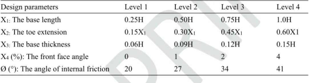
Table 1 - RC retaining wall design parameters and their levels.

Design parameters Level 1 Level 2 Level 3 Level 4

X1: The base length 0.25H 0.50H 0.75H 1.0H

X2: The toe extension 0.15X1 0.30X1 0.45X1 0.60X1

X3: The base thickness 0.06H 0.09H 0.12H 0.15H

X4 (%): The front face angle 0 1 2 4

Ø (°): The angle of internal friction 20 27 34 41

For designing the CRWs, wall height plays an important role in calculating the acting loads on the wall. Other parameters are the soil properties such as unit volume weight and angle of internal friction. Changes in the unit volume weights during optimal design do not affect the optimal weight values significantly; thus, γsoil = 18 kN/m3 was selected as the mean value

[22].Analysis parameters are the same for all CRW numerical analysis in GEO5 (Table 2). The safety factor of Fss was obtained by the Bishop method [21] via numerical analysis. For

numerical analysis, soil properties of the base soil and the backfill soil of the wall were the same. In the designs, only the weight of concrete was considered to identify the designs that satisfy the external stability conditions of the wall.

Table 2 - Analysis parameters for GEO5 numerical analysis.

Parameter Value

b: The top thickness of the stem 0.25 m

δ: The friction angle between base and soil (2/3) Ø

Df: The depth of the base X3

γsoil: The unit volume weight of soil 18 kN/m3

c: The cohesion of the soil 0

2.1. Taguchi Method

In this study, the Taguchi method [23], which is powerful and easily applicable, was employed to develop mathematical models of safety factors. This method gives the effects of the parameters as results within a short time and minimizes the effects of uncontrollable factors and limits the number of analysis required using orthogonal arrays; moreover, it reduces research cost and allows parametric analysis with fewer trials. In general, to examine the effect of five design parameters with four levels on the safety factors of Fs, Fo, and Fss,

1024 (45_{) designs must be examined. However, the Taguchi method makes it is possible to}

obtain the effect of parameters with only 16 designs using an orthogonal array. In this study, L16 orthogonal array which is given in the first column of Table 3 for five parameters with

four levels was employed.

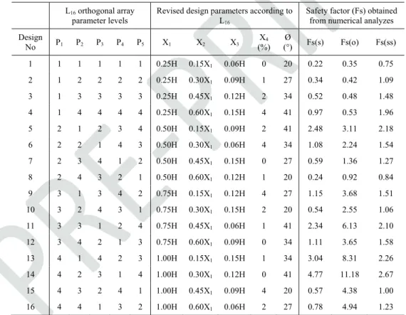
Table 3. L16 (45) orthogonal array, CRW Taguchi design table and results of numerical

analyses.

L16 orthogonal array

parameter levels

Revised design parameters according to

L16

Safety factor (Fs) obtained from numerical analyzes Design No P1 P2 P3 P4 P5 X1 X2 X3 _(%) X4 _(°) Ø Fs(s) Fs(o) Fs(ss) 1 1 1 1 1 1 0.25H 0.15X1 0.06H 0 20 0.22 0.35 0.75 2 1 2 2 2 2 0.25H 0.30X1 0.09H 1 27 0.34 0.42 1.09 3 1 3 3 3 3 0.25H 0.45X1 0.12H 2 34 0.52 0.48 1.48 4 1 4 4 4 4 0.25H 0.60X1 0.15H 4 41 0.97 0.53 1.96 5 2 1 2 3 4 0.50H 0.15X1 0.09H 2 41 2.48 3.11 2.18 6 2 2 1 4 3 0.50H 0.30X1 0.06H 4 34 1.08 2.24 1.54 7 2 3 4 1 2 0.50H 0.45X1 0.15H 0 27 0.59 1.36 1.27 8 2 4 3 2 1 0.50H 0.60X1 0.12H 1 20 0.24 0.92 0.84 9 3 1 3 4 2 0.75H 0.15X1 0.12H 4 27 1.15 3.68 1.51 10 3 2 4 3 1 0.75H 0.30X1 0.15H 2 20 0.54 2.55 1.06 11 3 3 1 2 4 0.75H 0.45X1 0.06H 1 41 2.34 6.13 2.10 12 3 4 2 1 3 0.75H 0.60X1 0.09H 0 34 1.11 3.65 1.58 13 4 1 4 2 3 1.00H 0.15X1 0.15H 1 34 3.04 8.31 2.26 14 4 2 3 1 4 1.00H 0.30X1 0.12H 0 41 4.77 11.18 2.67 15 4 3 2 4 1 1.00H 0.45X1 0.09H 4 20 0.57 4.38 1.00 16 4 4 1 3 2 1.00H 0.60X1 0.06H 2 27 0.78 4.94 1.23

Accordingly, the L16 design table was revised by using the design parameters and the levels

in Table 1 (the second column of Table 3). For obtaining this design table, 16 CRW designs were modeled and analyzed in the GEO5. At the end of those analyses, safety factors of

sliding, Fs(s), overturning, Fs(o), and slope stability, Fs(ss) were obtained and have been demonstrated as the results of numerical analyses in the last column of Table 3.

In the Taguchi method, the effects of the parameters on the results and the mathematical model are designated with a signal-to-noise (S/N) ratio described by Taguchi; it is used as the performance criterion in experiment design. The reduction of design parameter effects with the bigger S/N ratios can affect the result by decreasing the variance around the target value. The S/N ratios are classified into three types according to the purpose of the application: the smaller is better, the nominal is the best, and the larger is better (Equations 1 to 3, respectively). 2 S / N = -10 log( (Y ) / n) (1) 2 S / N = -10 l g(Y /o σ ) (2) 2 S / N = -10 log( (1 / Y ) / n) (3)

In these equations, Y is the response value, n is the number of repetitions, Ῡ is the arithmetic mean, and σ is the standard deviation. For developing a mathematical model statistically with Taguchi Method, better models were obtained using S/N ratios according to the target state “the larger is better” [24]. In this study, S/N analyses were performed according to the target state “the larger is better,” which maximizes the robustness. In the Statistica statistical software [25], S/N ratios were obtained using safety factors from numerical analyses in GEO5 and the change in the average S/N ratios according to parameter levels have shown in Figure 3 for each design parameters. In the CRW designs, the most effective parameter for the safety factors of Fs(s) and Fs(ss) is Ø, whereas that for the safety factor of Fs(o) is X1.

2.2. Mathematical Model

In this study, the average S/N ratios were employed to enhance the mathematical models for calculating the safety factors of sliding Fm(s), overturning Fm(o), and slope stability Fm(ss) and the general representation of the model for CRW height (H) of 6 m is given by Equation 4.

1

F_m = _{-λ /10}

10

(4)

where  is the total effect coefficient, which is explained by Equation 5.

λ = ψ_B + ψ_B + ψ_d + ψ_m + ψ_f + Δ

t ₍₅₎

Table 4 - The effect coefficients of parameters of Fm(s).

The lower-upper limits of parameters

Safety

factor Mathematical Model

(B/H) = 0.25–1.0 Fm(s) ψ = 18.486(B H⁄ ) − 42.672(B H⁄ ) + 43.961(B H⁄ ) − 14.9016 Fm(o) ψ = 31.275(B H⁄ ) − 86.36(B H⁄ ) + 98.437(B H⁄ ) − 31.9741 Fm(ss) ψ = −0.9481(B H⁄ ) + 1.104(B H⁄ ) + 3.1679(B H⁄ ) − 1.4958 (Bt/B) = 0.15–0.60 Fm(s) ψ = 28.534(B B⁄ ) − 32.262(B B⁄ ) − 0.1304(B B⁄ ) + 2.8788 Fm(o) ψ = −6.1339(B B⁄ ) − 4.6395(B B⁄ ) − 0.0334(B B⁄ ) + 2.5975 Fm(ss) ψ = −0.0165(B B⁄ ) − 1.1675(B B⁄ ) − 1.8(B B⁄ ) + 1.5046 (d/H) = 0.06–0.10 Fm(s) ψ = 334.17(d H⁄ ) − 39.307(d H⁄ ) + 15.177(d H⁄ ) − 1.8281 Fm(o) ψ = −226.44(d H⁄ ) + 46.681(d H⁄ ) − 12.536(d H⁄ ) + 2.376 Fm(ss) ψ = −2336.4(d H⁄ ) + 702.1(d H⁄ ) − 48.723(d H⁄ ) + 0.7493 m =0.00–0.04 Fm(s) ψ = 5415.9m + 950.03m − 46.71m + 0.0130 Fm(o) ψ = 26766m − 1478m + 15.336 m + 1.3036 Fm(ss) ψ = 43197m − 2498.5m + 37.666 m + 0.4955 Ø = 20°–41°

Fm(s) ψ = 23.23(tanϕ) − 51.682(tanϕ) + 67.598(tanϕ) − 26.9956

Fm(o) ψ = −2.4364(tanϕ) + 1.584(tanϕ) + 15.801(tanϕ) − 8.2024

Fm(ss) ψ = 14.299(tanϕ) − 38.059(tanϕ) + 45.098(tanϕ) − 15.4637

ψB : effect coefficient of the base length, X1(H)

ψBt : effect coefficient of the toe extension, X2(X1)

ψd : effect coefficient of the base thickness, X3(H)

ψm : effect coefficient of the front face angle, X4 (%)

The coefficient of Δ, which is the average S/N ratio, is considered as −1.034, 6.423, and 3.156 for Fm(s), Fm(o), and Fm(ss), respectively. Detailed mathematical explanations of all parameter-effect coefficients are provided in Table 4 for the safety factors of Fm(s), Fm(o), and Fm(ss). The values of all effect coefficients were defined between the lower and upper limits of design parameters listed in Table 1.

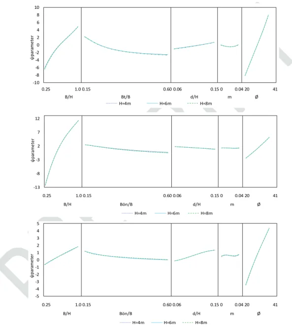
Figure 4 - The change between the effect coefficients of parameters and the different mathematical models for safety factors sliding, overturning and slope stability,

respectively. -10 -8 -6 -4 -2 0 2 4 6 8 10 ψ p aram e te r H=4m H=6m H=8m B/H Bt/B d/H m Ø 0.25 1.0 0.15 0.60 0.06 0.15 0 0.04 20 41 -13 -8 -3 2 7 12 ψ param et er H=4m H=6m H=8m B/H Bön/B d/H m Ø 0.25 1.0 0.15 0.60 0.06 0.15 0 0.04 20 41 -5 -4 -3 -2 -1 0 1 2 3 4 5 ψ p ar am e te r H=4m H=6m H=8m B/H Bön/B d/H m Ø 0.25 1.0 0.15 0.60 0.06 0.15 0 0.04 20 41

Mathematical models have statistically developed for H=4, 8 m by using the same way and the changes in the safety factor of the effect coefficient for each parameter according to wall height is shown in Figure 4. An examination of the figures clearly shows that the behavior of the effect coefficient is approximately the same for all wall heights. Thus, the mathematical model for H=6 m can be used in the CRW design with a range of H=4–8 m.

The safety factors of 1024 CRW designs, which involve all possibilities of five design parameters with four levels, were obtained by both numerical analysis and mathematical models for H = 6 m.

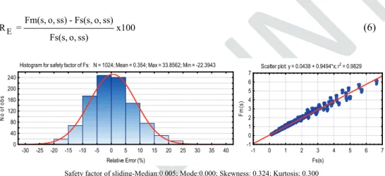
Relative errors (RE) of safety factors were calculated by Equation 6 and their histograms and

scatter plots for 1024 data have been constituted using relative errors (Figure 5).

E

Fm(s, o, ss) - Fs(s, o, ss)

R = x100

Fs(s, o, ss) (6)

Safety factor of sliding-Median:0.005; Mode:0.000; Skewness: 0.324; Kurtosis; 0.300

Safety factor of overturning-Median: −0.050; Mode:0.000; Skewness: −0.419; Kurtosis; 0.287

Safety factor of slope stability-Median: 0.000; Mode:0.000; Skewness: −0.390; Kurtosis; 0.287

Figure 5 - Histograms and scatter plots of relative errors for the safety factors Histogram for safety factor of Fs: N = 1024; Mean = 0.354; Max = 33.8562; Min = -22.3943

-30 -25 -20 -15 -10 -5 0 5 10 15 20 25 30 35 40 Relative Error (%) 0 40 80 120 160 200 240 N o o f obs Scatter plot: y = 0.0438 + 0.9494*x; r2 _{= 0.9829} -1 0 1 2 3 4 5 6 7 Fs(s) -1 0 1 2 3 4 5 6 7 Fm (s )

Histogram for safety factor of Fo: N = 1024; Mean = -0.1212; Max = 3.0604; Min = -4.8069

-6 -5 -4 -3 -2 -1 0 1 2 3 4 Relative Error (%) 0 50 100 150 200 250 300 350 N o o f obs Scatter plot: y = 0.163 + 0.915*x; r2 _{= 0.9997} -2 0 2 4 6 8 10 12 14 Fs(o) -2 0 2 4 6 8 10 12 14 Fm (o )

Histogram for safety factor of Fss: N = 1024; Mean = 0.1925; Max = 9.5423; Min = -11.7198

-14 -12 -10 -8 -6 -4 -2 0 2 4 6 8 10 12 Relative Error(%) 0 20 40 60 80 100 120 140 160 180 200 220 240 N o o f obs Scatter plot: y = -0.0332 + 1.0263*x; r2 _{= 0.9879} 0,0 0,5 1,0 1,5 2,0 2,5 3,0 Fs (ss) 0,4 0,8 1,2 1,6 2,0 2,4 2,8 3,2 F m (ss)

Note that the data set should follow a normal distribution when using the obtained mathematical model, i.e., the mean, median, and mode of the dataset coincide and that the coefficients of skewness and kurtosis of the data set are equal to zero. According to the criteria of the normal distribution of relative error histograms, which are presented in Figure 5, the mean, median, and mode are approximately coincident, and the coefficients of skewness and kurtosis are almost zero. The given criteria of histograms for the safety factors show that the relative error histograms of the obtained mathematical models have approximately normal distributions.

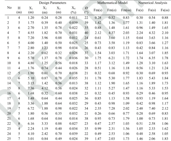
To control the mathematical models of safety factors, design parameters that satisfy the previously mentioned lower and upper limits were randomly selected. In all, 25 models of CRW were formed; this result differs from levels of design parameters given in Table 1. Table 5 lists all safety factors obtained from the mathematical model and numerical analyses with randomly selected parameters. Figure 6 shows the relative errors of the safety factors.

Table 5 - The cantilever retaining wall design results for 25 randomly data sets.

No

Design Parameters Mathematical Model Numerical Analysis

H (m) X1 (m) X2 (m) X3 (m) X4 (%) Ø (°) Fm(s) Fm(o) Fm(ss) Fs(s) Fs(o) Fs(ss) 1 4 1.20 0.24 0.28 0.011 22 0.28 0.52 0.83 0.30 0.54 0.88 2 5 1.75 0.39 0.40 0.039 39 1.42 1.36 1.77 1.31 1.40 1.81 3 6 2.70 1.35 0.78 0.022 35 0.88 1.48 1.61 0.96 1.49 1.65 4 7 4.55 1.82 0.70 0.031 40 2.12 4.37 2.03 2.24 4.32 2.10 5 8 7.20 3.96 0.88 0.012 24 0.61 3.60 1.15 0.64 3.63 1.16 6 5 4.00 1.40 0.50 0.025 25 0.73 3.58 1.19 0.83 3.66 1.27 7 7 2.80 1.23 0.98 0.034 26 0.43 0.83 1.13 0.42 0.84 1.16 8 4 2.20 0.62 0.32 0.028 37 1.54 3.03 1.71 1.64 3.07 1.85 9 6 5.70 1.37 0.78 0.036 30 1.75 6.21 1.72 1.74 6.35 1.78 10 8 4.80 1.25 0.56 0.018 33 1.17 3.12 1.49 1.28 3.10 1.63 11 4 1.76 0.74 0.44 0.026 28 0.51 1.16 1.18 0.56 1.21 1.24 12 5 1.90 0.61 0.70 0.038 21 0.32 0.68 0.92 0.30 0.69 0.93 13 6 5.10 0.87 0.78 0.035 31 1.78 5.30 1.77 1.83 5.43 1.84 14 7 3.15 1.42 0.56 0.013 38 1.12 1.90 1.65 1.16 1.89 1.73 15 8 7.36 4.12 0.56 0.024 32 1.11 5.27 1.47 1.16 5.33 1.53 16 6 1.68 0.32 0.60 0.038 23 0.32 0.45 0.93 0.29 0.46 0.95 17 4 1.48 0.64 0.44 0.025 36 0.85 1.13 1.58 0.93 1.19 1.64 18 8 3.36 1.88 0.64 0.032 29 0.43 0.98 1.09 0.42 0.98 1.17 19 7 6.72 1.88 0.98 0.022 34 2.35 7.28 2.02 2.48 7.40 2.12 20 5 1.80 0.56 0.35 0.032 21 0.26 0.66 0.77 0.28 0.69 0.83 21 6 1.68 0.64 0.84 0.014 38 0.95 0.73 1.79 1.00 0.73 1.81 22 8 6.16 3.33 0.88 0.027 23 0.47 2.57 1.03 0.51 2.58 1.06 23 4 2.24 1.19 0.40 0.034 35 0.99 2.31 1.56 1.05 2.33 1.62 24 5 4.10 2.42 0.70 0.039 22 0.49 2.53 1.06 0.48 2.58 1.05 25 7 3.01 0.84 0.49 0.024 39 1.47 2.03 1.73 1.46 2.06 1.83

According to Figure 6, the maximum absolute relative errors for the safety factors of Fs, Fo,

and Fss are viewed from the figure as 11.2%, 4.7%, and 8.7%, respectively. This result shows

that the developed mathematical models can be used with ~10% error for controlling CRW stability for the defined lower and upper limits of the design parameters.

Figure 6 - The values of relative errors of all safety factor for randomly selected 25 data set.

3. HARMONY SEARCH ALGORITHM

The harmony memory size (HMS) constitutes the basis of the HSA. The best example to explain HMS is a jazz group. Any jazz group comprises three musicians: a guitarist, a pianist and a drummer. Initially, three musicians keep different notes in their minds. For example, let the musicians think of playing the following notes randomly; e.g., the guitarist [Fa, Mi, Sol, Re, Si], the pianist [Si, La, Re, Sol, Do] and the drummer [Do, Fa, Sol, Re, Mi]. From these notes, let the guitarist plays Sol, the pianist plays Si, and the drummer plays Re. Thus, three musicians form a harmony as [Sol, Si, Re], which is called G-accord in music. If the harmony they generate in this way is better than the worst harmony in their memory, they eliminate the worst harmony from their memory and record the new harmony. They repeat this process until they identify that they have the best harmony. Hence, the relationship between HSA and design of a CRW can be established as follows. While the harmony in HSA represents the optimal CRW design, the different harmonies show the different feasible CRW designs. Each instrument acts for a design variable and so each note is represented by the base length (X1), the toe extension (X2), the base thickness (X3) and the front face angle

(X4) in the range given in Table 6. Finally, better harmonies correspond to local optimum

designs, and the best harmony corresponds to the global optimal design for a CRW design [6,26,27].

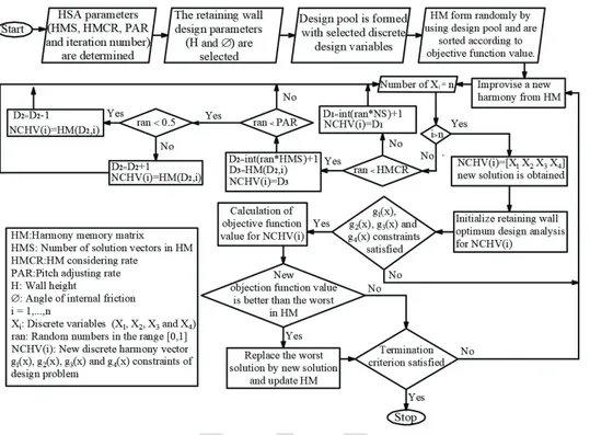
In Figure 7, a detailed flowchart is exhibited about the steps of the HSA to minimize the safety factors of a CRW with inequality constraints containing discrete design variables.

Figure 7 - Flowchart of the HSA for the optimum design of a CRW.

Moreover, the steps of the HSA can be interpreted in detail as follows:

Step 1: Initialization

The HSA parameters are initialized. The harmony search parameters can be defined as the harmony memory size (HMS), the harmony memory considering rate (HMCR), the pitch adjusting rate (PAR), and the maximum number of iterations (maxiter). Furthermore, in the

design problem, a potential value set is determined for each design parameter. The algorithm selects these values for determining the design variables from the design pool.

First, the values of HMS, HMCR, PAR and maximum iteration number have been identified for each feasible design. In this study, the parameters of the HSA are selected as HMS = 20, HMCR = 0.95, and PAR = 0.15. These parameter values are allocated at the beginning and they stay unchanged during the optimization process. The most suitable ranges for the parameters are specified by Geem et al [6]. When performing sufficient amount of runs for the sensitivity of the predetermined parameters, abovementioned HSA parameters are determined to utilize the least values of safety factors. To ensure the optimal values, which are obtained with the algorithm, the numerous iterations have been performed and the optimal values have been found within 10,000 iterations. For processing the optimal design, the optimal result remains the same after 5,000 iterations.

Step 2: Harmony memory matrix is initialized

A harmony memory matrix (HM) is formed and randomly filled with the first values. Each row of this matrix includes possible solution vectors and values, which are selected randomly from a design pool for that particular design variable. Therefore, the number of this row corresponds to the HMS. The HM matrix, shown in Equation 7, has N columns where N is the total number of the design variables of the optimization problem. In this equation, xi,j is

the value of the jth _{design variable that is randomly selected in the i}th _{possible solution (i =1,}

2,…., HMS and j = 1,2,…, N). In the ith _{possible solution, x}

i,j values are determined and the

objective function value corresponding to the present solution is calculated. After all harmony vectors have been calculated and are sorted in decrescent layout through their objective function value.

 

Step 3: Improvisation of a new harmony memory matrix

In the HSA, generating of a new harmony vector is realized according to three rules: (i) considering HM (HMCR), (ii) applying pitch adjustment (PAR), and (iii) using random selection (1-HMCR). For creating a new harmony matrix, the new value of the jth _design

variable is selected from the values stored in HM with the probability of HMCR, which varies between 0 and 1. In the random selection, the new value of the jth _{design variable is selected}

from the entire pool with the probability of (1-HMCR). Each design variable chosen from HM is then verified for whether it should be pitch-adjusted with the probability of PAR. HMCR and PAR are effective in determining global and local optimum designs, respectively.

Step 4: Harmony memory matrix is updated

After creating the recent solution (new harmony) vector, a new value for each design parameters have been obtained using the abovementioned three rules. So, the objective function value is calculated for the recent solution (new harmony) vector. This value is compared with the worst value of the objective function in HM. If it is better than the worst objective function, the recent solution vector is saved in HM and the worst design is eliminated. The HM is then sorted by the objective function value.

Step 5: Termination

Steps 3 and 4 are repeated until the criterion of termination (e.g., the maximum number of iterations) is satisfied. When the criterion of termination has been met, the algorithm is stopped.

4. OPTIMALLY FORMULATED CRW FOR PRE-DESIGN GUIDE

Investigation of the pre-design guide of the CRW, since calculating safety factors of Fs, Fo,

and Fss considering all combinations of the design parameters is tedious, the HSA is

employed to obtain results faster. The HSA which is the optimum design algorithm was encoded using MATLAB [28]. The general mathematical formation for optimal CRW design is identified below.

4.1. Design Parameters

In the optimal design problem, a design pool has been formed to solve the design problem with inequality constraints including discrete variables presented in Table 6. The lower and the upper bounds of them have been arranged according to mathematical models limits for design parameters. Because of the design parameters conform to the dimensions of CRW, these values and their intervals have been selected to be discrete to achieve integer wall sizes. This design pool contains information of the changing values of the base length, X1; toe

extension, X2; base thickness, X3; front face angle, X4; and constant values of the wall height,

H; and the angle of internal friction, Ø. X1, X2, X3 and X4 which increase from the lower limit

to the upper limit with the value of the interval have different sixteen, ten, seven and five values, respectively.

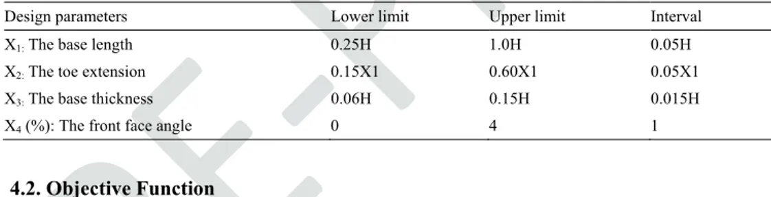
Table 6 Discrete design parameters and definition of limits.

Design parameters Lower limit Upper limit Interval

X1: The base length 0.25H 1.0H 0.05H

X2: The toe extension 0.15X1 0.60X1 0.05X1

X3: The base thickness 0.06H 0.15H 0.015H

X4 (%): The front face angle 0 4 1

4.2. Objective Function

Minimum values of safety factors (Fs, Fo, and Fss) were taken as the objective function with

the intent of obtaining safe and economic CRW design, which is used as the maximum capacity of stability. When the safety factors of the wall are the minimum but greater than 1.3 and close each other as much as possible, the maximum capacity of Fs, Fo, and Fss of the

wall is employed. In the case of using the maximum capacity of wall stability, it is possible to find implicitly economic wall design with obtaining close safety factors each other. In this study, unlike other studies conducted on CRW optimum design reported in the literature, a weighted-sum model as a multi-objective function has been employed to compute minimum safety factors value. Multi-objective function based on the weighted-sum model [29, 30] has been adopted as the sum of safety factors of sliding, overturning, and slope stability of CRW as given in Equation 8.

Here, Fm(s), Fm(o) and Fm(ss) are safety factors of sliding, overturning, and slope stability, respectively, and explained by Equations 4 and 5. According to the weighted-sum objective function model, the total value of coefficients a, b, and c should be 1.0. On the assumption that all safety factors have the same impact on the external stability of the wall, each of those coefficients is taken as 0.33.

4.3. Constraints

The design constraints for formulating the optimization problem are so-called safety factors of Fs, Fo, and Fss, as well as the geometric constraints of the wall. The lower and upper limits

of the safety factors against sliding, overturning, and slope stability are taken as 1.3 and 3.0 to yield the more economic wall design, respectively. In other words, it is intended to determine wall designs by providing the maximum capacity of stability. Maximum capacity of stability indicates that the wall design is safe (satisfy stability with safety factors greater than 1.3) and economic (with close safety factors each other and smaller than 3.0). In the optimization analyses, any designs having greater safety factors of Fs and Fss value than 1.3

could not be attained for any of lower internal friction angles (Ø < 24°). Wall designs that safety factor of Fo is smaller than 3.0 could not be obtained for Ø < 30°. Consequently, wall

designs could not be obtained, which satisfy both the lower and upper limits of safety factors for Ø =20°-30°. For these reasons, the lower and upper limits of safety factors for different values of Ø (°) used in the optimization process are designated in Table 7. They are also the values of limits for safety factors by which the feasible designs are obtained.

Table 7 - The lower-upper limits of safety factors of constraints.

Ø (°) Fm(s) Fm(o) Fm(ss)

Min Max Min Max Min Max

24 1.30 1.35 1.30 6.20 1.30 1.50

26 1.30 1.70 1.30 6.70 1.30 1.70

28 1.30 1.95 1.30 5.00 1.30 1.80

30−42 1.30 3.00 1.30 3.00 1.30 3.00

In the CRW design, the constraints are considered as normalized mathematical expressions as shown in Equation 9 and Equation 10 for the safety factor of Fs, in Equation 11 and

Equation 12 for the safety factor of Fo, and in Equation 13 and Equation 14 for the safety

factor of Fss. Moreover, the normalized geometric constraints of the wall are given in

Equation 15.

𝑔 (1) = 1 − (𝐹𝑚(𝑠)/𝐹𝑚(𝑠) ) ≤ 0 (9)

𝑔 (2) = (𝐹𝑚(𝑠)/𝐹𝑚(𝑠) ) − 1 ≤ 0 (10)

𝑔 (4) = (𝐹𝑚(𝑜)/𝐹𝑚(𝑜) ) − 1 ≤ 0 (12)

𝑔 (5) = 1 − (𝐹𝑚(𝑠𝑠)/𝐹𝑚(𝑠𝑠) ) ≤ 0 (13)

𝑔 (6) = (𝐹𝑚(𝑠𝑠)/𝐹𝑚(𝑠𝑠) ) − 1 ≤ 0 (14)

𝑔 (7) = . ∗ − 1 ≤ 0 (15)

4.4. Pre-Design Guide for Cantilever Retaining Wall

In this study, the HSA is implemented to just obtain an optimal pre-design guide for CRW in a short time. For the optimization process, after the initial selection of HSA parameters (HMS, HMCR, PAR, and maxiter), the wall height, the angle of internal friction, and the

design pool have been determined. The new wall design is obtained using values of the discrete design variables randomly selected from the design pool. In accordance to this new design, which surely satisfies the whole constraints as given in Equations 9–15, the minimum objective function (Equation 8) value and accordingly the wall dimensions have been obtained from all combinations for each case. Figure 8 shows the obtained minimum values of the CRW design parameters that the safety factors were greater than 1.3. All the safety factors of Fs, Fo, and Fss exceeded 1.3 for Ø ≥ 24° and were lesser than 3.0 for Ø ≥ 30°. The

CRW designs that satisfy the external stability condition of the wall were not obtained for Ø = 20° and 22°. Generally, designs with safety factors between 1.3 and 3.0 are obtained for Ø = 30°–42°. Except for Ø = 34° and Ø = 36° (X4=%3.00), the values of X4 were 0.00% for all

values of the angle of internal friction (Ø).

For realizing a pre-design guide for the CRW, 60 different cases, including five values of H (4, 5, 6, 7, and 8 m) and twelve values of Ø (20°, 22°, 24°, 26°, 28°, 30°, 32°, 34°, 36°¸38°, 40°, and 42°) were examined using HSA. Each case has been involved in 5600 (16 × 7 × 10 × 5) combinations for variable values of design parameters.

The proportional values of the design parameters (X1/H, X2/X1, and X3/H) and safety factors

remained constant despite changes in the wall height and the angle of internal friction. The optimum values of X4 and proportions of the wall dimensions for X1, X2, and X3 shown with

their safety factors in Figure 8 with average relative errors which were calculated using safety factors obtained from verification analysis conducted in GEO5 and safety factors of the optimum wall designs. Because changes in the design parameters exhibited similar behavior for all wall heights, the average relative errors given in Figure 8 are valid for all wall heights. In Table 8, suggested wall dimensions according to design codes for the base length, the toe extension, and the base thickness are demonstrated. The analysis results listed in Figure 8 were compared with the proposed wall dimensions based on the design codes (Table 8). When X1/H was examined for all wall heights, the proposed based length in design codes

(0.40 H- 0.75 H) was obtained for Ø = 28°, 30°, 32°, 34°, and 36°. The proposed base length according to the design codes was not obtained for other internal friction angles. Although the toe extension was proposed as 0.30X1 or 0.33X1, it was obtained generally as 0.15X1 for

approximately for only Ø = 40° in the analyses. Except for Ø = 38°, 40°, and 42°, the values of the base thickness were approximately 0.15H for all angles of internal friction. This value satisfies the in the proposed wall dimensions according to the design code of LRFD. Values of the base thickness for Ø = 38°, 40°, and 42° are close to those mentioned in the design code of ACI318. Because the base thickness in TS7994 is given as 80 cm, Figure 8 was used for comparison. For wall heights of 6, 7, and 8 m and angles of internal friction between 36° and 38°, the value of X3 is 80 cm. Consequently, it is not recommended to use the wall

dimensions based on the design codes from the viewpoint of economic design of CRW in soil with Ø < 30°.

Figure 8 - Suggestion of pre-design guide for the CR wall.

Table 8 - Suggested wall dimensions according to design codes.

Codes The base length The toe extension The base thickness

TS7994 [2] 0.40H–0.70H 0.33X1 80 cm

ACI318 [3] 0.40H–0.60H 0.33X1 0.07H–0.10H

LRFD [4] 0.70H*–0.75H* 0.30X1 0.10H–0.15H

H: The wall height, H*: The stem height

Because feasible solutions for Ø = 20° and 22° were not obtained in the analyzes, the numerical analyses in GEO5 were repeated to obtain the wall dimensions that satisfy the external stability conditions for the minimum safety factors (Table 9). In the same table, the

0.00 0.50 1.00 1.50 2.00 2.50 3.00 3.50 4.00 4.50 5.00 5.50 6.00 6.50 7.00 7.50 8.00 8.50 Ø = 24° Ø = 26° Ø = 28° Ø = 30° Ø = 32° Ø = 34° Ø = 36° Ø = 38° Ø = 40° Ø = 42° Ø = 24° Ø = 26° Ø = 28° Ø = 30° Ø = 32° Ø = 34° Ø = 36° Ø = 38° Ø = 40° Ø = 42° Ø = 24° Ø = 26° Ø = 28° Ø = 30° Ø = 32° Ø = 34° Ø = 36° Ø = 38° Ø = 40° Ø = 42° X1 X2 X3 W al l dim es io n (m ) H=4m H=5m H=6m H=7m H=8m X1 (H) X2 (X1) X3 (H) (X1 / H) (X2 / X1) X3 / H 24 1 0.2 0.15 0 1.3 5.46 1.43 -12 1 4 26 0.85 0.15 0.15 0 1.3 4.3 1.51 -5 1 8 28 0.75 0.15 0.15 0 1.35 3.67 1.6 -3 0 8 30 0.6 0.15 0.15 0 1.31 2.6 1.64 -2 -2 9 32 0.5 0.15 0.15 0 1.32 1.95 1.71 -3 -1 9 34 0.45 0.15 0.135 3 1.3 1.72 1.79 1 1 12 36 0.4 0.25 0.15 3 1.31 1.4 1.88 3 2 14 38 0.35 0.2 0.075 0 1.32 1.33 1.72 -5 2 12 40 0.35 0.35 0.075 0 1.33 1.35 1.78 -6 3 12 42 0.35 0.5 0.06 0 1.31 1.33 1.8 -14 4 11

Minimum safety factors Average relative errors (%)

Ø (°) _(%)X4 Fm (s) Fm (o) Fm (ss) Fs Fo Fss

proportional values of wall dimensions were obtained with the safety factors of Fs(s), Fs(o), and Fs(ss). From Table 9, it is seen that the designs that satisfied the minimum stability conditions of CRW does not have economic wall dimensions because of obtained great base length and safety factor of Fo. Moreover, despite changes in the wall heights, proportional

wall dimensions stay constant. When the safety factors for Ø = 20° and 22° are examined, the value of Fs(o) is higher than the values of Fs(s) and Fs(ss). Consequently, an economic design is not possible when the internal friction angle of soil is either 20° or 22°.

Table 9 - Results for satisfied stability conditions of CRW designs in GEO5.

H (m) X1 (m) X1/H X2 (m) X2/X1 X3 (m) X3/H X4(%) Fs(s) Fs(o) Fs(ss) Ø=20° 4 6.60 1.65 1.32 0.20 0.60 0.15 0.00 1.33 12.87 1.54 5 8.30 1.65 1.65 0.20 0.75 0.15 0.00 1.32 12.85 1.48 6 9.90 1.65 1.98 0.20 0.90 0.15 0.00 1.32 12.84 1.47 7 11.60 1.65 2.31 0.20 1.05 0.15 0.00 1.32 12.84 1.49 8 13.20 1.65 2.64 0.20 1.20 0.15 0.00 1.32 12.83 1.41 Ø=22° 4 5.60 1.40 1.12 0.20 0.60 0.15 0.03 1.35 9.98 1.53 5 7.00 1.40 1.40 0.20 0.75 0.15 0.03 1.35 9.96 1.51 6 8.40 1.40 1.68 0.20 0.90 0.15 0.03 1.34 9.95 1.52 7 9.80 1.40 1.96 0.20 1.05 0.15 0.03 1.34 9.95 1.52 8 11.2 1.40 2.24 0.20 1.20 0.15 0.03 1.34 9.94 1.52

The proposed wall dimensions of CRW for wall heights of 4, 5, 6, 7, and 8 m and different values of angle internal friction are shown in Figure 9, Figure 10, Figure 11, Figure 12, and Figure 13, respectively. It is possible to perform CRW design by using these figures. For example, the design of wall for H = 6 m and Ø = 30°, the obtained wall dimensions are X1 =

3.6, X2 = 0.54, and X3 = 0.90 m according to Figure 11. In these figures, while the safety

factors of Fs, Fo, and Fss are in the range of 1.3–3.0 for Ø = 30°, 32°, 34°, 36°, 38°, 40°, and

42°, they are just greater than 1.3 for Ø =24°–30°. In other words, for wall designs in soil with Ø < 30°, a safety factor of overturning smaller than 3.0 is not obtained using these figures.

Ultimately, the obtained all CRW designs were examined in terms of soil bearing capacity using Terzaghi bearing capacity theory [31] for the strip foundation. The results show that soil bearing capacity of the obtained all CRW designs is provided except for Ø = 24°. Therefore, the proposed pre-design guide designated in Table 10 is included the CRW designs for H = 4, 5, 5, 6, 8 m and Ø = 26°, 28°, 30°, 32°, 34°, 36°, 38°, 40°, 42°. Using values of the minimum design parameters given in Table 10, some sample CRW designs have been analyzed for different conditions of soil and slope in GEO5, and they have been listed in Table 11. The ultimate bearing capacities (qu, kN/m3) of the base soil have been

calculated for wall designs. Then, safe bearing capacities (qs, kN/m3) for SF= 3.0, and

maximum values of base pressure distribution (σmax) of the wall designs have been calculated,

Figure 9 - Suggestions of wall dimensions for H =4 m.

Figure 11 - Suggestions of wall dimensions for H =6 m.

Figure. 13 Suggestions of wall dimensions for H =8 m

Table 11 shows that safe bearing capacities (qs) of the base soil are greater than the maximum

value of base pressure distribution (σmax) of example wall designs. When safety factors of

Fs(s), Fs(o), and Fs(ss), as well as criteria of bearing capacity of wall designs in table are examined, safety factors are greater than 1.3 and loads from the base to the soil are safely transmitted for the minimum suggested wall dimensions. The results show that the suggested design table (Table 10) can be used for designing a CRW for determined values of angle of internal friction and wall height.

5. CONCLUSIONS

In this study, a pre-design guide depending on soil properties was improved using the HSA for a CRW. The lower and upper limits of the wall dimensions were assigned following TS7994, ACI 318, and LRFD design codes such that the wall dimensions obtained from the analyses could be compared with those proposed based on the design codes. The base length, X1; the toe extension, X2; the base thickness, X3; the front face angle, X4; and the angle of

internal friction, Ø were considered as the design parameters with their varied values. To verify the external stability of the CRW, the safety factors of Fs, Fo, and Fss were

considered. For calculating the safety factors, mathematical models were improved by a statistical method according to the determined design parameters. In developing the mathematical model, the safety factors of sliding Fs(s), overturning Fs(o), and slope stability Fs(ss), as obtained from CRW designs, were used and analyzed in GEO5.

As the wall designs did not satisfied stability conditions such as sliding, overturning, slope stability, and bearing capacity for Ø = 20°, 22°, and 24°, the results were not added in the pre-design guide. For all combinations of variable values of design parameters, it needs to be checked whether the constraints have been satisfied and which one has the minimum objective function value. For this case, the formulations of safety factors derived from mathematical models were used as design constraints and objective function to obtain safe and economic CRW designs, the lower constraint limit was set as 1.3 and the upper constraint limit as 3.0. HSA provides the optimal result in a short time for obtaining the minimum value of the objective function in the analyses. The wall height (H) and the angle of internal friction (Ø) were considered as a constant parameter in each HSA-based optimization analyses. Analyses were performed for each value of H and Ø, and the wall dimensions (X1, X2, X3,

X4) satisfying the upper and lower limits were determined. The obtained results and

suggestions are as follows:

Finding absolute average relative errors of improved mathematical models for safety factors of Fs, Fo, and Fss as 6.4%, 1.0%, and 2.8%, respectively, shows that these models may be

reliably used for determining safety factors. Coefficients of determination (r2_{) have been}

found as 0.99 for the abovementioned mathematical models from scatter plots.

While feasible solutions with safety factors greater than 1.3 were not obtained for Ø = 20° and 22°, the criteria of bearing capacity of proposed wall designs were not satisfied for Ø = 24°. Because soils with Ø < 24° are not sufficient to provide the safety factors of Fs and Fss

for the CRW, reasonable wall designs that satisfied the lower limit (1.3) of the constraints were not obtained for these values of Ø. Hence, when the angle of internal friction of backfill and foundation soil was lesser than 26°, it is recommended that the soil be improved or a different type of retaining structure such as CRW with keys or steps or counterfort wall be used.

CRW designs were not obtained for the safety factor of Fo smaller than 3.0 for Ø < 30°.

Consequently, safe and economic CRW designs may be obtained for soil with Ø > 30° such that the lower limit (1.3) and upper limit (3.0) are satisfied.

The proposed wall dimensions for the aforementioned design codes were not achieved for loose sand soil (Ø < 30°). According to the results, the use of the designs codes of T7994, ACI 318, and LRFD for the design of CRW is not recommended in soils with Ø < 30°. Soil properties have not been considered in the proposed wall dimensions according to the current design codes [2, 3, 4]. Safe and economic wall designs can be obtained using the proposed pre-design guide for CRW that incorporates varied values of angles of internal friction and wall heights are presented in this paper.

Eventually, a pre-design guide for CRW design was realized for conditions such as H = 4, 5, 6, 7, and 8 m; Ø = 30°, 32°, 34°, 36°, 38°, 40°, and 42°; and γsoil = 18 kN/m3.

In future, the scope of this study may be extended by considering different types of retaining walls and soil and slope properties.

Symbols

b The top thickness of the stem

bb The bottom thickness of the stem

B The base length

c Cohesion of soil

CRW Cantilever retaining wall

Df Depth of base

fmin Objective function

Fs General representation for sliding safety factor

Fo General representation for sliding safety factor overturning

Fss General representation for sliding safety factor slope stability

Fs (s) Sliding safety factor of numerical analysis

Fs (o) Overturning safety factor of numerical analysis

Fs (ss) Slope stability safety factor of numerical analysis

Fm (s) Sliding safety factor mathematical model

Fm (o) Overturning safety factor mathematical model

Fm (ss) Slope stability safety factor mathematical model

gx(1) The constraint of the minimum sliding safety factor

gx(2) The constraint of the maximum sliding safety factor

gx(3) The constraint of the minimum overturning safety factor

gx(4) The constraint of the maximum overturning safety factor

gx(5) The constraint of minimum slope stability safety factor

gx(6) The constraint of maximum slope stability safety factor

gx(7) Geometric constraints of the wall

H Wall height

HM Harmony memory matrix

HMCR Harmony memory considering the rate

HMS Harmony memory size

HSA Harmony search algorithm

i The row number of HM

j Column number of HM

L16 Orthogonal array

maxiter Maximum number of iterations

N Total number of the design variables

n Number of repetitions

PAR Pitch adjusting rate RE Relative Error r2 _{Coefficients of determination} S/N Signal/Noise ratio Y Response value Ῡ Arithmetic mean X1 Base length X2 Toe extension X3 Base thickness

X4 Front face angle

Δ Coefficient of the average S/N ratio

δ Friction angle between base and soil

Ø The angle of internal friction

γsoil Unit volume weight of soil

γconcrete Unit volume weight of concrete

ψB Effect coefficient of the base length, X1(H)

ψBt Effect coefficient of the toe extension, X2(X1)

ψd Effect coefficient of the base thickness, X3(H)

ψm Effect coefficient of the front face angle, X4 (%)

ψØ Effect coefficient of the angle of internal friction, Ø (°)

 Total effect coefficient

σ Standard deviation

Acknowledgements

In this study, results of a part of the continuing doctoral thesis have been submitted and also it is supported by Scientific Research Projects Coordination Units of Selcuk University Research Funding (BAP- 17401107) which are gratefully acknowledged.

References

[1] Coduto, D., Geotechnical Engineering: Principles and PracticesPrentice-Hall, New Jersey, pp. 528–552. 1999.

[2] Turkish Standards Institute, Soil Retaining Structures; Properties and Guidelines for Design (TS 7994), Turkish Standard, 1990.

[3] American Concrete Institute, ACI Committee, and International Organization for Standardization, Building Code Requirements for Structural Concrete (ACI 318-14), 2014.

[4] McCormac, J. C., Brown, R. H., Design of Reinforced Concrete, John Wiley and Sons, 2015.

[5] Minnesota Department of Transportation Bridge Office, LRFD Bridge Design Manual, 5-392, 11-52, 2016.

[6] Geem, Z. W., Kim, J. H., Loganathan, G.V., A New Heuristic Optimization Algorithm: Harmony Search, Simulation, 76, 2, 60-68, 2001.

[7] Saka, M., Çarbaş, S., Optimum Design of Single Layer Network Domes Using Harmony Search Method, Asian Journal of Civil Engineering (Building and Housing), 10, 1, 97-112, 2009.

[8] Geem, Z. W., Optimal Cost Design of Water Distribution Networks Using Harmony Search, Engineering Optimization, 38, 3, 259-277, 2006.

[9] Geem, Z. W., Lee, K. S., Park, Y., Application of Harmony Search to Vehicle Routing, American Journal of Applied Sciences, 2, 12, 1552-1557, 2005.

[10] Cheng, Y. M., Li, L., Fang, S. S., Improved Harmony Search Methods to Replace Variational Principle in Geotechnical Problems, Journal of Mechanics, 27, 1, 107-119, 2011.

[11] Fattahi, H., Prediction of Slope Stability State for Circular Failure: A Hybrid Support Vector Machine with Harmony Search Algorithm, International Journal of Optimization in Civil Engineering, 5, 1, 103-115, 2015.

[12] Khajehzadeh, M.; Taha, M.R.; El-Shafie, A., Eslami, M., Economic Design of Foundation Using Harmony Search Algorithm, Australian Journal of Basic and Applied Sciences, 5, 6, 936-943, 2011.

[13] Akın, A., Saka, M. P., Optimum Design of Concrete Cantilever Retaining Walls Using the Harmony Search Algorithm, Proceeding of 9th International Congress on Advances in Civil Engineering Civil-Comp Press, 27-30, 2010.

[14] Uray, E., Çarbaş, S., Erkan, İ.H., Tan, Ö., Optimum Design of Concrete Cantilever Retaining Walls with the Harmony Search Algorithm, 6th Geotechnical Symposium, Turkey, 2015.

[15] Yepes, V., Alcala, J., Perea, C., González-Vidosa, F., A Parametric Study of Optimum Earth-Retaining Walls by Simulated Annealing, Engineering Structures, 30, 3, 821– 830, 2008.

[16] Molina-Moreno, F., García-Segura, T., Martí, J. V., Yepes, V., Optimization of Buttressed Earth-Retaining Walls Using Hybrid Harmony Search Algorithms, Engineering Structures, 134, 205-216, 2017.

[17] Rhomberg, E. J., Street, W. M., Optimal Design of Retaining Walls, Journal of the Structural Division, 107, 5, 992-1002, 1981.

[18] Keskar, A. V., Adidam, S. R., Minimum Cost Design of a Cantilever Retaining Wall, Indian Concrete Journal, 63, 8, 401-405, 1989.

[19] Saribas, A., Erbatur, F., Optimization and Sensitivity of Retaining Structures, Journal of Geotechnical Engineering, 122, 8, 649-656, 1996.

[20] GEO5, Geotechnical Design Computer Program, Fine Software, https://www.finesoftware.eu.

[21] Bishop, A. W., The Use of the Slip Circle in the Stability Analysis of Slopes, Geotechnique, 5, 1, 7-17, 1955.

[22] Uray, E., Çarbaş, S., Erkan, İ. H., Tan, Ö., Parametric Investigation for Discrete Optimal Design of a Cantilever Retaining Wall, Challenge Journal of Structural Mechanics, 5, 3, 108-120, 2019.

[23] Taguchi, G., Elsayed, E. A., Hsiang, T. C., Quality Engineering in Production Systems, McGraw-Hill, New York. 173, 1989.

[24] Tan, Ö., Investigation of Soil Parameters Affecting the Stability of Homogeneous Slopes Using the Taguchi Method. Eurasian Soil Science, 39, 11, 1248-1254, 2006. [25] Statistica, Statistical Analyses Computer Program, TIBCO Software Inc.,

https://www.tibco.com/products/tibco-statistica.

[26] Çarbaş, S., Saka, M. P, Optimum Topology Design of Various Geometrically Nonlinear Latticed Domes Using Improved Harmony Search Method, Structural and Multidisciplinary Optimization. 45, 3, 377-399, 2012.

[27] Lee, K. S., Geem, Z. W., A New Structural Optimization Method Based on the Harmony Search Algorithm, Computers and Structures, 82, 9, 781-798, 2004.

[28] Matlab R2017b, a programing language, MathWorks.

[29] Fishburn, P.C., Additive Utilities with Incomplete Product Set: Applications to Priorities and Assignments. ORSA Publication, Baltimore, 1967.

[30] Triantaphyllou, E., Multi-Criteria Decision-Making Methods. In Multi-Criteria Decision-Making Methods: A Comparative Study. Springer, Boston, MA, 5-21, 2000. [31] Terzaghi, K., Theoretical Soil Mechanics, 4th ed., John Wiley & Sons, Inc., New York,