The role of openness on the effectiveness of monetary policy: Experience of developing countreis in the 1990s

The Role of Openness on the Effectiveness of Monetary

Policy:

Experience of Developing Countries in the 1990s

Nihat Işık

Karamanoglu Mehmetbey Univ., Faculty of Economics and Administrative Sciences, Department of Economics

Mustafa Acar∗∗∗∗

Kırıkkale Univ., Faculty of Economics and Administrative Sciences, Department of Economics

Abstract

This paper attempts to examine how is the relationship between monetary policy and exchange rates affected by the openness of an economy, using annual data for a panel of twenty developing countries for the period of 1988-2000. The results show that the openness of an economy has a negative impact on the effectiveness of the monetary policy on the exchange rates. This result, which does not seem to be sensitive to exchange rate regimes enforced by the governments, indicates that an increase in the money growth rate leads to a smaller depreciation in the currency of developing countries with more open economies.

Keywords: Monetary Policy, Exchange Rate, Openness, Developing

Countries

Para Politikasının Etkililiği Üzerinde Açıklığın Rolü:

1990’larda Gelişmekte Olan Ülke Deneyimi

Özet

Bu çalışmada, para politikası ve döviz kuru arasındaki ilişkinin ekonominin açıklık derecesi tarafından nasıl etkilendiği incelenmektedir. Bu amaçla, 1988-2000 yılları arası 20 gelişmekte olan ülkenin birleştirilmiş verileri kullanılmıştır. Elde edilen bulgular, ekonominin açıklık derecesinin, para politikasının döviz kurları üzerindeki etkililiğini negatif yönde etkilediğini göstermektedir. Bu sonuç, devlet müdahalaesinin olduğu döviz kuru rejimlerinde de değişmemektedir. Buna gore, para arzının büyüme oranındaki artış, görece daha açık gelişmekte olan ülkelerin paralarında daha düşük oranda bir değer kaybına yolaçmaktadır.

Anahtar Kelimeler: Para Politikası, Döviz Kuru, Açıklık, Gelişmekte Olan

Ülkeler

*

Mustafa Acar, Corresponding Author, Address: Kırıkkale Üniversitesi, İİBF, İktisat Bölümü, Kırıkkale, Turkey, Email: ma@mustafaacar.com

1. Introduction

It is generally accepted that monetary expansions lead to depreciation of the domestic currency, while monetary contractions have the opposite effects.1 _{A number of previous studies support these predictions.}2 However, while monetary expansions are expected to result in depreciation of the national currency, the size of this depreciation may increase or decrease with the degree of openness of the economy.

Let us consider two economies with different degree of openness, one is more and the other is less open. An increase in money supply is expected to create similar effects in both economies on the demand side. Monetary expansion increases aggregate demand in two ways: first by decreasing interest rates, hence stimulating investment expenditures. Second, it increases demand through exchange rate depreciation (Berument and Doğan, 2003).

Depreciation makes domestic goods cheaper and imported goods more expensive, thereby improving net exports, hence output. Romer (1993) also provides some theoretical reasoning behind the difference between more and less open economies in terms of inflationary effects.

It is likely to create quite different effects on the supply side, as well. Due to the consequent depreciation following a monetary expansion, demand for an increase in wages in a highly open economy will be more vigorous than a relatively closed one. This follows from the fact that changes in the value of domestic currency will affect agents of a highly open economy more seriously. More vigorous wage increases will steepen aggregate supply. Consequently, more of the monetary expansion will be reflected more on prices and less on output. The opposite will be true for a relatively less open economy.3

Exchange rate has been regarded as one of the key transmission mechanisms through which monetary expansion affects the economic activity, in addition to the other three channels—interest rate, asset price, and credit—(Mishkin, 1995). As Dennis (2001) puts it, on the financial side, exchange rates are key variables in small open economies. Changes in exchange rate directly influence the prices of tradable goods. As

1

In this study exchange rate is defined as units of domestic currency against one unit of foreign currency.

According to this definition, an increase in exchange rate indicates depreciation, i.e. a fall in the value of domestic currency.

2

Among others, see for example Bryant et al. (1988), Taylor (1993), Dornbusch and Giovannini (1994).

3 _{See Karras (1996) for some empirical tests supporting these relationships for} output and prices.

domestic currency depreciates,4 _{imported consumer goods become more} expensive, raising the consumer price index. Prices of imported intermediate goods also go up, increasing the cost of production of firms. Higher production costs tend to increase prices of consumer goods further as firms try to pass on higher costs to consumers. On the real side, a fall in the real value of domestic currency stimulates world demand for domestically produced goods, leading to an improvement in the trade balance.

One should note that theoretical as well as empirical literature so far has focused more on the effects of changes in money supply on the exchange rate, neglecting the role of openness. Karras’ leading paper (1999) highlighted the role of openness on the ability of monetary policy to affect the exchange rate. Using annual data for 1953-1990 period for a panel of 38 countries, he investigated the relationship amongst exchange rate, openness and monetary policy. His empirical results indicated that the more open the economy, the smaller is the depreciation effects of a given change in the money supply.

Following Karras (1999), in this paper we want to explore the same issue for the case of developing countries. We would like to see if empirical evidence from developing countries for a different period will support theoretical expectations as well as Karras’ findings. Furthermore, we would like to see if the results are sensitive to exchange rate regimes. In this regard, this paper analyzes empirically the role of openness on the exchange rate effects of monetary policy by using annual data for a panel of 20 countries5 for the period of 1988-2000. The primary criterion used to select a country was whether she has followed open policies based on free market economy or not. The twenty developing countries chosen for empirical analysis have been determined by using IMF country classification. The rest of the paper is organized as follows: The following section introduces the model and the data.

Section 2 presents and discusses the empirical results. Conclusions follow.

2. The Model, the Data and Methodology

In this study, the following model is estimated in order to demonstrate the relationship between exchange rate and money growth rate.

4

In this paper, exchange rate is defined as how many units of domestic currency one has to pay for 1 unit of foreign currency. In this definition an increase in exchange rate indicates a decrease in the value of domestic currency.

5

The following countries are included in the analysis: South Korea, Hungary, Mexico, Poland, Turkey, Argentina, Brazil, El Salvador, Honduras, Panama, Paraguay, Uruguay, Venezuela, South Africa, Egypt, Tunisia, Indonesia, India, Philippines, and Israel.

∑

= − + + = s i er t j i t j m t j i t j m er 0 , , , , 0 ,

β

β

ε

(2.1)

Where, subscripts j and t refer to countries and years, respectively. β denotes coefficients.

Error terms are modeled as the fixed effects. Rate of changes, rather than levels, of the values of the variables have been used to have a better comparison amongst the countries. The rate of change in exchange rates and the money supply are defined as follows, respectively:

erj,t=( Ej,t-Ej,t-1) / Ej,t-1

mj,t=(M2Yj,t-M2Yj,t-1)/M2Yj,t-1

Following Karras (1999), the equation below has been used to link money supply with openness in an effort to show the effects, depending on the degree of openness, of monetary policies on the exchange rates.

t j i m i m t j i,,

θ

θ

δ

,

β

=

+

δ (2.2)

Here, θs are parameters, and δj,t measures the degree of openness in country j at time t. The following equation is obtained when equation (2.2) is plugged into equation (1.1).6

(

)

∑

= − − + + + = s i er t j i t j t j i i t j m i t j m m er 0 , , , , 0 ,

β

θ

θ

δ

ε

δ _(2.3)

Equation (2.3) is estimated in order to evaluate the role of openness on the ability of monetary expansions to affect exchange rate. Where the dependent variable er_j,t denotes the rate of change in the exchange rate of country j in period t, m_j,tdenotes the rate of change in M2Y of country j in period t.

δ

_j,tm_j,t is the interaction term and shows the effect of monetary policy on exchange rate depending on the degree of openness.

Since foreign currency deposits are also taken into account, broad definition of money, M2Y, is thought to be a better proxy for money supply changes for the purpose of this study.7

The data are obtained from IMF’s International Financial Statistics. Openness can be defined in various ways by using various measures. Among these are exports plus imports over GDP, imports over GDP, trade orientation, degree of interest rate differentiation between countries, and degree of capital mobility. In empirical studies the first two criteria have been the most widely used openness measures (Romer, 1993; Rane, 1997; Edwards, 2001; Karras, 1999; Berument and Doğan, 2002; Akçay, 2000).

6

See Karras (1999) for a formal derivation on how openness is likely to influence the exchange rate effects of monetary policy.

7 _{M2Y = Money in circulation + Demand deposits + Time deposits + Deposits in} foreign currency.

This study employs the first three measures to represent the degree of openness. The first two are taken from the literature mentioned above. δ1, is defined as (imports+exports)/GDP. The second openness measure, δ2, includes only imports (imports/GDP). In addition to these two, this study uses a third measure, δ3, as a proxy for trade orientation, and it was obtained by following Balassa and Bauwens (1988).8

Interaction between money growth rate (m) and openness measures are represented by γ1, γ2 and γ3 and defined as follows:

γ1= (δ1*m), γ2= (δ2*m), γ3= (δ3*m)

As far as the model specified in Equation (2.3) is concerned, the coefficient

θ

iδ shows whether the effects of monetary policy on the exchange rate is strengthened with openness (

_θ

δ

i > 0), or weakened ( δ

θ

_i < 0). Theoretically, the sign of

θ

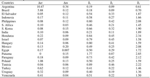
_iδis uncertain9, hence it remains as an empirical question to be explored.

Table 1 shows sample means over 1988-2000 for each currency’s annual depreciation rate (∆er) with respect to the U.S. dollar, each country’s annual money growth rate (∆m), as well as the three openness measures (δ1, δ2 and δ3) for each country.

Table 1: Sample Means of the Series over 1988-2000

Notes: ∆er is the depreciation rate of the local currency with respect to the U.S. dollar; ∆m is the

growth rate of M2Y, δ1 is the sum of exports plus imports as a fraction of GDP, δ2 is imports as a

fraction of total consumption.

8 _{This last measure is used to define openness in a broader sense. It is suggested} by Balassa and Bauwens, and calculated as the residuals obtained by regressing logarithmic values of per capita imports on logarithmic values of per capita gross domestic product. These residuals that are taken to be proxies for trade orientation represent those variables affecting imports.

9 _{See Karras (1999) for a formal derivation of this relationship, which shows the} ambiguity of the sign of the openness coefficient.

Countries ∆er ∆m δ1 δ2 δ3 Argentina 10.47 0.34 0.19 0.09 0.61 Brazil 5.88 0.12 0.18 0.09 0.70 El Salvador 0.05 0.12 0.54 0.33 1.87 Indonesia 0.17 0.11 0.58 0.27 1.66 Philippines 0.08 0.12 0.80 0.42 2.08 S. Africa 0.10 0.03 0.46 0.21 1.45 S. Korea 0.08 0.15 0.66 0.32 1.90 India 0.10 0.06 0.21 0.11 1.89 Honduras 0.22 0.09 0.84 0.45 2.34 Israel 0.07 0.09 0.79 0.45 1.58 Hungary 0.14 0.06 0.80 0.41 1.59 Mexico 0.13 0.20 0.49 0.25 2.08 Egypt 0.17 0.007 0.50 0.29 1.72 Panama 0 0.15 1.77 0.87 2.85 Paraguay 0.18 0.09 0.73 0.42 2.12 Poland 1.08 0.13 0.50 0.25 1.59 Tunisia 0.04 0.06 0.89 0.46 2.22 Turkey 0.62 0.12 0.41 0.22 1.46 Uruguay 0.32 0.09 0.40 0.19 1.36 Venezuela 0.41 0.04 0.51 0.22 1.50

Looking at columns 1 and 2 of Table 1, one can see that changes in exchange rates and money supply substantially differ across countries. For instance, the average annual depreciation rate has ranged from 4% for Tunisia, to 1047% for Argentina, whereas annual money growth rates have ranged from 4% for Venezuela, and 34% for Argentina.

Last three columns in Table 1 show the sample means of three openness measures (δ1, δ2 and δ3) for each country. For these three measures, the lower is the sample means; the less open is the country. In that respect, even though we have obtained almost the same results for first two measures of openness, the third one, a proxy for trade orientation, has given us quite different results. For example, Panama is the most open country in terms of all three measures, while second and third most open countries are Tunisia and Honduras for first measure, Honduras and Tunisia for third measure, respectively. By the same token, fourth, fifth and sixth most open countries are Hungary, Philippines and Israel for first measure, and Paraguay, Meksika and Philippines for third measure, respectively. Finally, as the least open country is Brazil and then Argentina for first two measures, for third measure it is vice versa, i.e. the least open is Argentina and then Brazil.

3. Empirical Results

Equation (2.3) will be estimated using panel data. The term panel

data refers to data sets where we have data on the same individual over

several periods of time. In the panel data analysis, time series and cross-sectional data series are combined together and data sets which have both time and section dimensions are formed. The reiterations of cross-section observations with respect to years are likely. Therefore, panel data analysis basically depends on repeated analyses of variance (ANOVA) and models of ANOVA.

A panel data regression differs from a regular time series or cross-section regression in that it has a double subscript on its variables, i.e.

it it it X u y ' + + =

α

β

i = 1, 2, ……., N; t = 1, 2, ….., T (3.1)

with i denoting households, individuals, firms, countries, etc. and t denoting time. The i subscript, therefore, denotes the cross-section dimension whereas t denotes the time-series dimension. α is a scalar, β is Kx1 and Xit is the ith observation on K explanatory variables (Baltagi, 2003: 12).

One of the early uses of panel data in economics was in the context of estimation of production functions as in Hoch (1962) and Mundlak (1961, 1963), where allowance had to be made for unobserved effects specific to each production unit. The model used is now referred to as fixed effects model (Maddala, 1987: 303) and is given by,

y_{it = i +} 'X_{it +}u_it

β

The only difference between equation (3.2) and equation (3.1) is that coefficient α takes subscript i in equation (3.2). Hence, this will allow fixed term α to change and to take into account the specific variation and differences such as different country sizes, work experiences and individual abilities. The other method used in estimation of panel data analysis and first applied by Balestra ve Nerlove (1966) is random effect model. In this model, αi just like uit in equation (3.2) is considered as random variable. There are different views in the literature on which of these two procedures should be used.

In this context, if factors (in this study, countries) are chosen arbitrarily then fixed effects is used, while random effects would be more appropriate when factors are chosen randomly. Similarly, fixed effects is preferred if inferences obtained from the model are limited to the sample, whereas random effects is more appropriate if the inferences are to be generalized (Hsiao, 1986). Also Judge and others (1985) showed that the fixed effect estimator is more appropriate under more general assumptions. Hausman’s (1978) specification test is widely used to determine whether to use fixed or random effect procedure in the estimation of parameters. Hausman test statistic asymptotically shows a χ2 distribution under the null hypothesis “random effects estimator is correct” with K degrees of freedom.

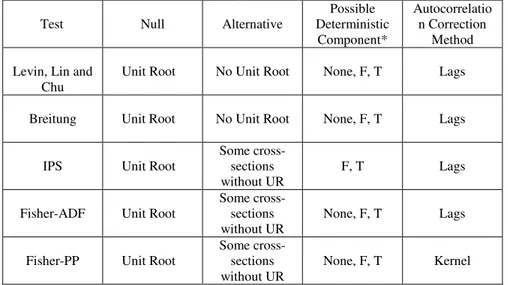
Panel unit root tests have been done to elicit time-series properties of variables and to enable reliable parameter results. Panel unit root tests are similar, but not identical, to unit root tests carried out on a single series. Recent literature suggests that panel-based unit root tests have higher power than unit root tests based on individual time series (Im, Peseran and Shin, 2003, Breitung, 2000). In that respect, five different panel unit root tests have been calculated: Levin, Lin and Chu (2002), Breitung (2000), Im, Pesaran and Shin (2003), Fisher-type tests using ADF and PP tests (Maddala and Wu (1999). On the other hand, “Common root” indicates that the tests are estimated assuming a common AR structure for all of the series; “Individual root” is used for tests which allow for different AR coefficients in each series. Table 2 summarizes the basic characteristics of the some panel unit root tests.

Table 2: Basic characteristics of the some panel unit root tests

Test Null Alternative

Possible Deterministic Component* Autocorrelatio n Correction Method Levin, Lin and

Chu

Unit Root No Unit Root None, F, T Lags

Breitung Unit Root No Unit Root None, F, T Lags

IPS Unit Root

Some cross-sections without UR

F, T Lags

Fisher-ADF Unit Root

Some cross-sections without UR

None, F, T Lags

Fisher-PP Unit Root

Some cross-sections without UR

None, F, T Kernel

*None - no exogenous variables; F - fixed effect; and T - individual effect and individual trend. Panel unit root test results have been derived for each variable in the models (Table 3).

Table 3: Panel Unit Root Test Results

Null: Unit root (assumes common unit root process) Exchange Growth Rate (e) (Export+Import) / GDP (γ1) (Import) / GDP (γ2) Trade Orientation (γ3) Money Growth Rate (m)

Method Statistic Statistic Statistic Statistic Statistic

Levin, Lin &

Chu t* -472.988 -10.5400 -7.54330 -9.80613 -11.4716

Breitung t-stat -2.57311 -4.63814 -4.55353 -4.61620 -3.69163

Null: Unit root (assumes individual unit root process) Im, Pesaran and Shin W-stat -179.067 -7.28124 -6.01683 -6.94341 -7.47488 ADF - Fisher Chi-square 183.043 121.239 104.818 116.450 122.613 PP - Fisher Chi-square 168.920 137.692 140.744 149.475 149.326

** Probabilities for Fisher tests are computed using an asympotic Chi-square distribution. All other tests assume asymptotic normality.

Based on the results, it is clear that there is no panel unit root in any of the variables. Having done panel unit root tests for each variable, parameters have been estimated. Based on Hausman test results, country specific fixed effect procedure is used in all models in this study. Furthermore, Generalized Least Squares estimation method, which uses

cross section as weights, has been used in all models. White Heteroskedasticity-Consistent Standart Errors&Covariance have been taken into consideration, as well. Estimation results obtained by using fixed effects procedure are reported in Table 4.10

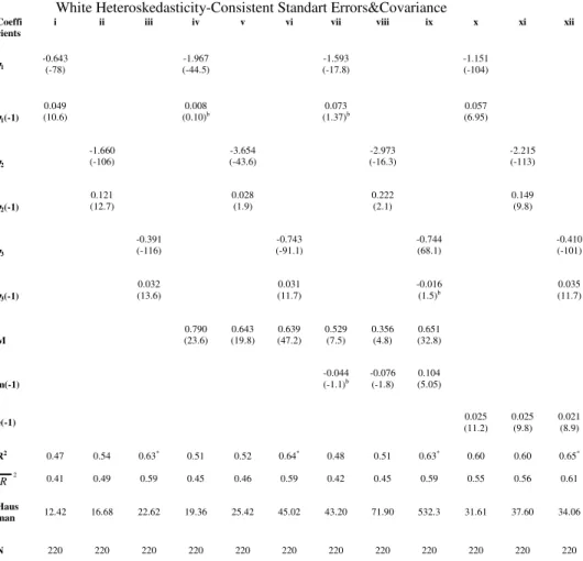
Table 4: Estimation Results (Dependent variable: exchange rate growth, e; all countries:

1988-2000)a

Method: GLS (Cross Section Weights)

White Heteroskedasticity-Consistent Standart Errors&Covariance

a _{Figures in parentheses are t statistics. All estimates are statistically significant at 5 percent except for}

having superscript b.

* _{Notice that the third openness criterion generates higher R}2 _{results implying that trade orientation has}

better explanatory power.

As can be followed from Table 4, the coefficients γ1, γ2 and γ3 in each model showing the interaction between openness and money supply are found to be negative and statistically significant. These results indicate that

10 _{Fixed effects obtained from the models are available from the authors upon} request.

Coeffi

cients i ii iii iv v vi vii viii ix x xi xii

γγγγ1 -0.643 _(-78) -1.967 _{(-44.5) (-17.8)} -1.593 -1.151 _(-104) γγγγ1(-1) 0.049 (10.6) 0.008 (0.10)b _(1.37)0.073 b 0.057 _(6.95) γγγγ2 -1.660 (-106) -3.654 (-43.6) -2.973 (-16.3) -2.215 (-113) γγγγ2(-1) 0.121 (12.7) 0.028 (1.9) 0.222 (2.1) 0.149 (9.8) γγγγ3 -0.391 (-116) -0.743 (-91.1) -0.744 (68.1) -0.410 (-101) γγγγ3(-1) 0.032 (13.6) 0.031 (11.7) -0.016 (1.5)b 0.035 _(11.7) M 0.790 (23.6) 0.643 (19.8) 0.639 (47.2) 0.529 (7.5) 0.356 (4.8) 0.651 (32.8) m(-1) -0.044 (-1.1)b -0.076 _{(-1.8) (5.05)} 0.104 e(-1) 0.025 _(11.2) 0.025 _(9.8) 0.021 _(8.9) R2 _{0.47 0.54 0.63}* _{0.51 0.52 0.64}* _{0.48 0.51 0.63}* _{0.60 0.60 0.65}* 2 R 0.41 0.49 0.59 0.45 0.46 0.59 0.42 0.45 0.59 0.55 0.56 0.61 Haus man 12.42 16.68 22.62 19.36 25.42 45.02 43.20 71.90 532.3 31.61 37.60 34.06 N 220 220 220 220 220 220 220 220 220 220 220 220

the higher the level of openness, the lower the effects of money supply changes on the exchange rate, which confirms Karras’ results.

This negative relationship implies that openness reduces the ability of monetary policy to affect exchange rates. As a result, in more open economies, depreciation effects of a given money supply shock will be lower.

The values for the coefficient m, which represents money growth rate in the models, are estimated to be positive and significant in all model specifications. Consistent with theoretical expectations, greater money supply shocks lead to larger depreciation in the domestic currency. One point of curiosity is whether this result is sensitive to exchange rate regime. In an effort to explore this possibility, we estimated the model after excluding countries with pegged regimes.11 _{Table 5 reports the new} estimation results.

Table 5: Estimation Results (Dependent variable: exchange rate growth, e; countries with

flexible regimes:1988- 2000)a _{(Except for Argentina and Panama)}

Method: GLS (Cross Section Weights)

White Heteroskedasticity-Consistent Standart Errors&Covariance

a_{Figures in parentheses are t statistics. All estimates are statistically significant except for having superscript b.} * _{Notice that the third openness criterion generates higher R}2 _{results implying that trade orientation has better}

explanatory power.

11 _{Argentina and Panama were the only two countries which implemented fixed} exchange rate regimes throughout the whole period.

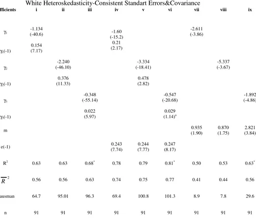
Coefficients i ii iii iv v vi vii viii ix

γ1 -1.056 (-133) -0.988 (-13.75) -1.748 (-57.12) γ1(-1) 0.023 _{(4.62) (11.93)}-0.134 _(3.52)0.384 γ2 -2.134 _{(-149) (-17.45)} -2.509 _(-60.67) -3.446 γ2(-1) _(11.76) 0.103 _(-13.43) -0.322 _(3.56) 0.751 γ3 -0.431 _{(-118) (-24.75)} -1.184 _(-43.61) -0.594 γ3(-1) 0.025 (9.49) -0.004 (-1.03)b 0.160 _(3.72) M _(0.09)0.005 b _(1.01)0.054 b _(15.36) 1.409 e(-1) _0.291 (4.95) 0.278 (4.80) 0.298 (4.06) R2 0.60 0.61 0.66* _{0.43 0.49 0.58}* _{0.64 0.66 0.67}* 2 R _{0.55 0.57 0.62 0.37 0.43 0.53 0.60 0.62 0.63} Hausman 23.52 31.72 25.52 17.76 21.77 11.78 293.6 142.8 442.3 N 198 198 198 198 198 198 198 198 198

As can be seen from Table 5, values of γ1, γ2 and γ3 in the models are estimated to be negative and significant. These results indicate that, in terms of both individual and combined effects for all models, generally the higher the openness, the lower the effect of monetary expansion on exchange rate. Note that the results do not substantially differ between Table 4 and Table 5, which implies that it is not the exchange rate regimes that drive the results.

The parameter values for money growth (m) in the models are estimated to be all positive and significant. This implies that monetary expansions lead to depreciation of domestic currency for developing countries. The reason behind this finding may be explained as follows. Monetary expansions lead to a fall in interest rates. This is not surprising, because, in an open economy with liberalized capital account, this stimulates capital flight, which causes domestic currency to depreciate (Dornbusch and Fischer, 1994). In the standard textbook IS-LM model, LM shifts to the right as a result of money growth, interest rates fall, and then two channels operate which eventually causes domestic currency to depreciate. In the first one, falling interest rates stimulates output through increased investments. Rising income deteriorates trade balance by raising imports, which leads to balance of payments deficits. Domestic currency is expected to depreciate to improve trade balance. The second one has to do with capital flight. Falling interest rates stimulates capital flight as a result of investors’ turning outside markets for higher returns on their capital. Falling demand for domestic currency coupled with increasing demand for foreign currency causes domestic currency to depreciate (Yıldırım and Doğan, 2001:243).

Given the fact that some of the developing countries adopted fixed exchange rate regimes during late 1980’s and early 1990’s, one might think of one further robustness check: exclude those developing countries with pegged regimes up to 1993, after which, only Argentina and Panama remained as fixed regimes. Therefore, we excluded 5 more countries from the sample and repeated the analysis. Table 6 gives estimation results for 1993-2000 where all countries in the sample strictly implemented flexible exchange rate regimes—excluding all 7 countries with pegged regimes partly or fully during 1988-1992. 12

Note that openness terms are negative and significant, whereas money terms are positive and significant in the models above. Once again, these results are consistent with the expectations: monetary expansions lead to depreciation, openness reduces the ability of monetary policy to affect

12 _{Argentina, Panama, El Salvador, Honduras, Israel, Hungary and Poland were} seven countries which implemented fixed exchange rate regimes throughout the 1988-1992 period.

exchange rate. The higher the openness, the lesser is the rate of depreciation of domestic currency due to monetary expansion.

Regression results with different specifications consistently indicated two main findings: Openness reduces the ability of monetary policy to affect exchange rate, and monetary expansions result in depreciation of domestic currency for developing countries. The results confirm the previous empirical findings of Karras (1999) in terms of the role of openness in affecting the ability of monetary policy on changes in exchange rates.

Table 6: Estimation Results (Dependent variable: exchange rate growth, e; countries with

flexible exchange rate regimes 1993-2000)a _{(Except for 7 countries)}

Method: GLS (Cross Section Weights)

White Heteroskedasticity-Consistent Standart Errors&Covariance

a _{Statistically insignificant.}

* _{Notice that the third openness criterion generates higher R}2 _{results implying that trade orientation has}

better explanatory power.

4. Conclusion

This paper examines whether the effects of monetary policy on the exchange rates depend on the degree of openness of an economy. Economic theory suggests that the effect of openness on the ability of money to influence the exchange rate is ambiguous. This relationship is

Coefficients i ii iii iv v vi vii viii ix

γ1 _(-40.6) -1.134 -1.60 (-15.2) -2.611 (-3.86) γ1(-1) 0.154 (7.17) 0.21 (2.17) γ2 -2.240 (-46.10) -3.334 (-18.41) -5.337 (-3.67) γ2(-1) 0.376 (11.33) 0.478 (2.82) γ3 -0.348 (-55.14) -0.547 (-20.68) -1.892 (-4.86) γ3(-1) 0.022 (5.97) 0.029 (1.14)a m _(1.90)0.935 _(1.75)0.870 _(3.84) 2.821 e(-1) _(7.74) 0.243 _(7.77) 0.244 _(8.17) 0.247 R2 _{0.63 0.63 0.68}* _{0.78 0.79 0.81}* _{0.50 0.53 0.63}* 2 R 0.56 0.56 0.63 0.74 0.75 0.77 0.41 0.44 0.56 Hausman 64.7 95.01 96.3 69.4 100.8 101.3 8.9 7.8 29.6 n 91 91 91 91 91 91 91 91 91

investigated by using panel data of 20 developing countries for 1988-2000 period.

The estimation results indicate that openness reduces the impact of monetary policy on exchange rate. Whether they adopt fixed or flexible exchange rate regimes, there is a negative relationship between the degree of openness and the effect of money growth on exchange rate.

Another finding is that monetary expansions lead to depreciation of domestic currency for developing countries. We found that for developing countries as a whole, i.e. independent from the nature of the exchange rate regimes, money growth leads to depreciation. This relationship holds for developing countries with flexible regimes as well for the same period, which implies that monetary expansion leading to depreciation does not depend on exchange rate regime.

These empirical findings suggest that the influence of monetary policy on exchange rate decreases as an economy becomes more open. In developing countries local currency depreciates as money supply grows. These findings are in conformity with theoretical expectations as well as a number of previous empirical studies.

References

Akçay, S. (2000), “Yolsuzluk, Ekonomik Özgürlükler ve Demokrasi”, (Corruption, Economic Freedoms and Democracy), Muğla Üniversitesi Sosyal Bilimler Enstitüsü

Dergisi, (Muğla University Journal of Social Sciences Institute) Fall 2000, 1(1): 1-15. Balassa, B. and L. Bauwens (1988), Changing Trade Patterns in Manufactured

Goods, An Econometric Investigation, Amsterdam: North Holland.

Balestra, P. and M. Nerlove (1966), “Pooling cross-section and time series data in the estimation of a dynamic model: the demand for natural gas, Econometrica, Vol. 34: 585-612.

Baltagi, B. H. (2003), Econometric Analysis of Panel Data, Second Edition, John Wiley&Sons, Ltd., England.

Berument, H. (2002), “Döviz Kuru Hareketleri ve Enflasyon Dinamiği: Türkiye Örneği,” (Exchange Rate Movements and Inflation Dynamics: Turkish Case,) Bilkent

University Discussion Papers, No: 02-02, March 2002, pp. 1-14.

Berument, H. and B. Doğan (2003) “Openness and the Effectiveness of Monetary Policy: Empirical Evidence from Turkey,” Applied Economics Letters, 10: 217-221.

Breitung, Jörg (2000). “The Local Power of Some Unit Root Tests for Panel Data,” in B. Baltagi (ed.), Advances in Econometrics, Vol. 15: Nonstationary Panels, Panel

Cointegration, and Dynamic Panels, Amsterdam: JAI Press, p. 161–178.

Bryant, R., D. Henderson, G. Holtham, P. Hooper, S. Symansky (1988), Empirical

Macro-economics for Interdependent Economies, Washington, DC: Brookings Institution. Dennis, R. (2001) “Monetary Policy and Exchange Rates in Small Open Economies,”

FRBSF Economic Letter, 16(May):1-4.

Dornbusch, R., A. Giovannini (1990), “Monetary Policy in the Open Economy,” in B.M. Friedman and F.H. Hahn (eds.) Handbook of Monetary Economics, New York: North Holland.

Dornbusch, R., S. Fischer (1994), Macroeconomics, Sixth Edition, Singapore: McGraw-Hill.

Edwards, S. (2001), “Dollarization: Myths and Realities,” National Bureau of

Fleming, J.M. (1962), “Domestic Financial Policies Under Fixed and Under Floating Exchange Rates,” IMF Staff Papers, Vol. 9: 369-376.

Hausman, J. (1978), “Specification Tests in Econometrics,” Econometrica, Vol. 46: 1251-1271.

Hoch, I. (1962), “Estimation of production function parameters combining time-series and cross-section data,” Econometrica, Vol.30: 34-53.

Hsiao, C. (1986), Analysis of Panel Data, Cambridge: Cambridge Univ. Press. Im, K. S., Pesaran, M. H., and Y. Shin (2003). “Testing for Unit Roots in Heterogeneous Panels,” Journal of Econometrics, 115, 53–74.

Judge, G.G, W.E. Griffiths, R.C. Hill, H. Lutkepohl, T.C. Lee (1985), The Theory

and Practice of Econometrics, New York: John Wiley.

Kamin, S.B. and J.H. Rogers (2000) “Output and Real Exchange Rate in Developing Countries: An Application to Mexico,” Journal of Developing Economics, 62: 85-109.

Karras, G. (1999), “Monetary Policy and the Exchange Rate: The Role of Openness,”

International Economic Journal, 13(2): 75-88.

Karras, G. (1996), “Are the Effects of Monetary Policy Asymmetric? Evidence from a Panel of European Countries,” Oxford Bulletin of Economics and Statistics, May: 267-278.

Levin, A., Lin, C. F., and C. Chu (2002). “Unit Root Tests in Panel Data: Asymptotic and Finite-Sample Properties,” Journal of Econometrics, 108, 1–24.

Maddala, G. S. (1987), “Recent Developments in the Econometrics of Panel Data Analysis,” Transportation Research, Vol. 21: 303-326.

Maddala, G. S. and S. Wu (1999). “A Comparative Study of Unit Root Tests with Panel Data and A New Simple Test,” Oxford Bulletin of Economics and Statistics, 61, 631– 52.

Mishkin, Frederic S. (1995) “Symposium on the Monetary Transmission Mechanism,” Journal of Economic Perspectives, 9(4): 3-10.

Mundell, R.A. (1962), “The Appropriate Use of Monetary and Fiscal Policy for Internal and External Stability,” IMF Staff Papers, Vol. 9, March: 70-77.

Mundlak, Y. (1961), “Empirical production functions free of management bias,”

Journal of Farm Economics, Vol. 43: 44-56.

Mudlak, Y. (1963), Estimation of production and behavioral functions from a

combination of cross-section and time-series data, In Measurement in Economics, Edited by C. F. Christ, Stanford University Press, Stanford.

Obstfeld, M. ve K. Rogoff (1996), Foundations of International Macroeconomics, Cambridge: MIT Press.

Rane, Philip R. (1997), “Inflation in Open Economies,” Journal of International

Economics, Vol. 42: 327-347.

Romer, D. (1993), “Openness and Inflation: Theory and Evidence,” Quarterly

Journal of Economics, Vol. 108: 869-903.

Taylor, John B. (1993), Macroeconomic Policy in a World Economy, New York: Norton.

Yıldırım, K. and D. Karaman (2003), Makroekonomi (Macroeconomics), Eskişehir: Eğitim Sağlık ve Bilimsel Araştırma Çalışmaları Vakfı.