GLOBAL ALIGNMENT OF METABOLIC PATHWAYS AND PROTEIN-PROTEIN INTERACTION NETWORKS
GRADUATE THESIS
GAMZE ABAKA
Ga mze Ab aka M.S . The si s 2014 S tudent’ s F ull Na me P h.D. (or M.S . or M.A .) The sis 20 11
INTERACTION NETWORKS
by Gamze Abaka
Bachelor’s degree, Computer Engineering, Kadir Has University, 2012
Submitted to the Graduate School of
Science and Engineering in partial fulfillment of the requirements for the degree of Computer Engineering
Master of Science
Kadir Has University 2014
ABSTRACT
GLOBAL ALIGNMENT OF METABOLIC PATHWAYS AND
PROTEIN-PROTEIN INTERACTION NETWORKS
Metabolic pathways and protein interaction networks are essential at almost every func-tion for living organisms. Simply, while reacfunc-tions produce life energy within cells, protein interaction networks provide biological functions. Also, abnormal reactions or interactions cause various disorders. Thus, in bioinformatics, most of the studies are based on these net-works in order to find hopeful results for these disorders and biological challenges. Solving alignment problem is one of these studies such that it tries to find similar reactions, proteins or functions. In this thesis, we focus on that problem within both metabolic pathways and protein interaction networks. Firstly, we propose a constrained alignment algorithm, CAM-Pways, for one-to-many alignment of metabolic pathways and we extend the framework, CAPPI, for one-to-one protein interaction network alignment with necessary changes. Af-terwards, we provide the computational intractability of the problem and finally we compare our algorithm with different algorithms on actual metabolic pathways and protein interaction networks.
¨
OZET
METABOL˙IK YOLAKLARIN VE PROTE˙IN ETK˙ILES
¸ ˙IM
A ˘
GLARININ H˙IZALANMASI
Metabolik yolaklar ve protein etkile¸sim a˘gları ya¸sayan canlıların neredeyse t¨um fonksiy-onlarnda hayati ¨onem ta¸smaktadır. En basit haliyle, reaksiyonlar h¨ucre i¸cinde ya¸sam enerjisi ¨
uretirken, protein etkile¸sim a˘gları biyolojik fonksiyonların ger¸cekle¸smesini sa˘glamaktadır. Ayrca, normal olmayan reaksiyonlar ya da etkile¸simler ¸ce¸sitli hastalıklara neden olmak-tadır. Bu nedenle, biyoinformatik alanındaki bir ¸cok ¸calı¸sma, bu hastalıklara ve biyolo-jide ¸c¨oz¨ulmesi gereken sorunlara umut verici sonu¸clar alabilmek amacıyla, bu a˘glara dayan-maktadır. Hizalama probleminin ¸c¨oz¨ulmesi, bu ¸cal¸smalardan biridir ve bu problem, ben-zer reaksiyonları, proteinleri ya da fonksiyonları bulmaya ¸cal¸sır. Bu tez kapsamında, hem metabolik yolaklar hem de protein etkile¸sim a˘gları i¸cin hizalama problemi ele alınmaktadır.
¨
Oncelikle metabolik yolakların bire-¸cok hizalanması i¸cin kısıtlandırılmı¸s bir algoritma (CAM-Pways) sunulmakta, daha sonra bu algoritma protein etkile¸sim a˘glarının bire-bir hizalanması i¸cin geli¸stirilmekte (CAPPI) ve gerekli de˘gi¸siklikler uygulanmaktadır. Problemin i¸slemsel karma¸sıklı˘gı verilip, ger¸cek veriler ¨uzerinde di˘ger algoritmalar ile kar¸sla¸stırmaları yapılmaktadır.
ACKNOWLEDGEMENTS
It is my great pleasure to thank many people who helped me for my studies and inspired me for my life. Firstly, I would like to thank Assoc. Prof. Cesim ERTEN, my thesis advisor, for his valuable and constructive suggestions. Also, I would like to offer my special thanks to him for endearing bioinformatics area to me.
I am particularly grateful for the assistance given by research assistances, my friends.
Especially, many thanks to Aykut C¸ ayır for his helps about programming knowledge and
Serkan Altunta¸s for his valuable ideas and inspirations about bioinformatics and biological processes. I would also thank to all computer engineering professors for their worthful courses and my high school teacher S¸enay ¨Ozt¨urk for her inspiration.
I would like to express my very great appreciation to my family and my close friends. I thank my parents Nermin & Do˘gan Abaka for their endless confidence and support. Finally, I would like to thank my friends Barı¸s Karata¸s, C¸ i˘gdem ¨Ozt¨urk, Kadir ¨Ozbek and Seda C¸ am and all my other friends who inspire me.
TABLE OF CONTENTS
ABSTRACT . . . iii ¨ OZET . . . iv ACKNOWLEDGEMENTS . . . v LIST OF FIGURES . . . ix LIST OF TABLES . . . x 1. INTRODUCTION . . . 1 1.1. Metabolic Pathways . . . 11.1.1. Metabolism and Metabolic Reactions . . . 1
1.1.2. Significance of Metabolism . . . 3
1.1.3. Metabolic Pathways and Their Functions . . . 4
1.2. Protein-protein Interaction Networks . . . 7
1.3. Network Alignment Problem . . . 10
1.3.1. Global and Local Alignment Problem . . . 11
1.3.2. Pairwise and Multiple Alignment Problem . . . 12
1.4. The Scope and Contribution of the Thesis . . . 13
2. METHODS AND ALGORITHMS . . . 14
2.1. Problem Definition for Metabolic Pathway Alignment . . . 14
2.2. Constrained Alignment Framework . . . 16
2.3. CAMPways Algorithm . . . 18
2.3.1. Constructing Bipartite Similarity Graph . . . 18
2.3.2. Conflict Graph Generation and Conflict Resolution . . . 20
2.3.3. Final Alignment Expansion . . . 24
2.4. Extension of Constrained Alignment Framework and CAMPways Algorithm 24 2.4.1. Problem Definition for PPI Network Alignment . . . 25
2.4.3. Finding Maximum Weight Bipartite Matching . . . 26
2.4.4. Constructing Reduced Bipartite Similarity Graph . . . 27
2.4.5. Conflict Graph Generation and Conflict Resolution . . . 28
2.4.6. Final Alignment Expansion . . . 31
3. COMPLEXITY ANALYSIS . . . 32
3.1. NP-Hardness Proof of Constrained Alignment Problem . . . 32
3.2. Polynomial Time Solution of the Alignment Problem . . . 35
4. DISCUSSION OF RESULTS . . . 36
4.1. Discussion of Results for CAMPways . . . 36
4.1.1. Reverse Engineering Metabolic Pathways . . . 37
4.1.1.1. Same-domain Alignments . . . 38
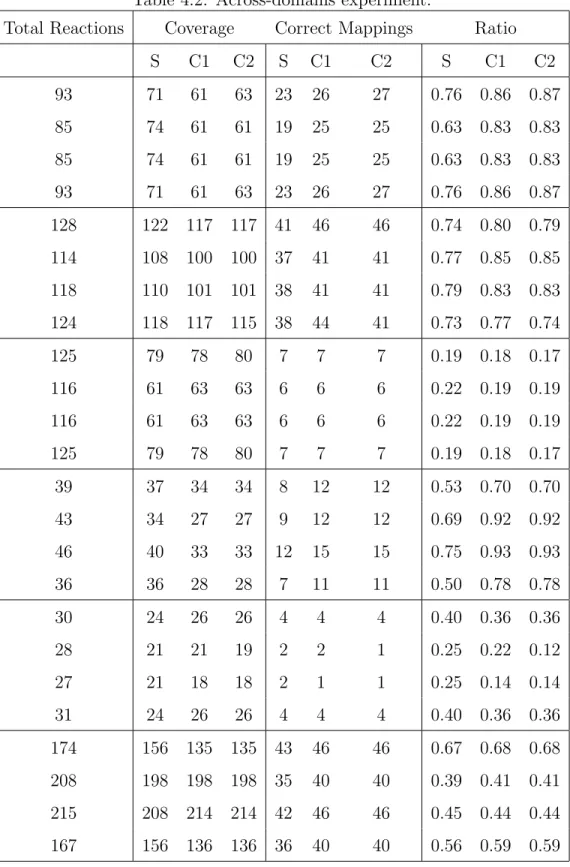
4.1.1.2. Across-domain Alignments . . . 40
4.1.1.3. Correctness and Sizes of Mappings . . . 41
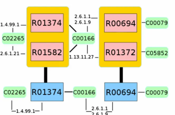
4.1.2. Biochemical Significance of the Alignments . . . 42
4.1.3. Execution Speed and Memory Requirements . . . 45
4.1.4. Running Time Analysis . . . 47
4.1.5. Discussion of Results for CAPPI . . . 48
REFERENCES . . . 57
LIST OF FIGURES
Figure 1.1. A metabolic pathway (taken from [1]) . . . 5
Figure 1.2. A protein interaction network (taken from [2]) . . . 8
Figure 2.1. CAMPways algorithm . . . 19
Figure 3.1. NP-Hardness Proof Graph . . . 33
Figure 4.1. Top: Same-domain (hsa-mmu). Bottom: Across-domains (hsa-atc) . . . 41
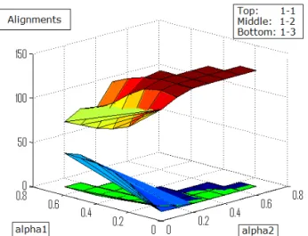
Figure 4.2. Same-domain (hsa-mmu) results. Top: 1-to-1 mappings. Middle: 1-to-2 mappings. Bottom: 1-to-3 mappings . . . 42
LIST OF TABLES
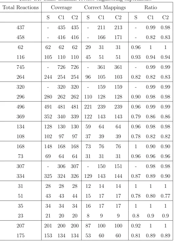
Table 4.1. Same-domains reverse engineering experiment. . . 50
Table 4.2. Across-domains experiment. . . 51
Table 4.3. Same-domains biochemical significance experiments. . . 52
Table 4.4. Across-domains biochemical significance experiments. . . 53
Table 4.5. Running Time Analysis Table . . . 54
Table 4.6. GOC evaluations . . . 55
1.
INTRODUCTION
The main purpose of biology is to understand the cell system such that the fundamen-tal questions can be answered: How the cellular functions happen and which interactions are established, in particular, how the proteins interact with each other to perform proper functions and how the reactions occur to maintain essential processes in the cell.
In this introductory chapter, there exist three main sections such that in the first section, the definition of metabolic pathways is given in order to indicate the significance of the subject. Afterwards, the notions that are used for the implementation of these pathways
in the alignment problems are given. In the second section, protein-protein interaction
networks and their notions are defined as well, and finally in the third main section, network alignment problem is described as a summary for a better understanding of the subject.
1.1. Metabolic Pathways
In this section, we give definitions of metabolic pathways, reactions and metabolic networks with the significance of them in the bioinformatics and we define the notions for a better understanding of the next problem sections.
1.1.1. Metabolism and Metabolic Reactions
In order to show the big picture of the metabolism by providing the important aspects of the subject, we first need to begin from the smallest piece of the metabolism: A chemical reaction is an occurrence of the interaction of two or more chemical substances that have accurate characteristic properties, and a transformation of them to others. Generally, the transformation separates the reactions as catabolic and anabolic. Whereas catabolic reactions
provide Adenosine triphosphate (ATP) that refers to chemical energy is usually used for the occurrence of new reactions such as anabolic reactions within cells and metabolism of living organisms by breaking down the complex organic molecules into smaller ones such as breaking down the sugar to obtain energy, anabolic reactions use the provided energy by catabolic reactions and gather the small molecules together to obtain complex organic molecules such as attaining protein by gathering the amino acids together. Both catabolic and anabolic reactions can happen at any moment but when the living organism is young, the number of anabolic reactions is greater than the number of catabolic reactions for growth and the living organism gets older, firstly the number of catabolic reactions balances with the number of anabolic reactions and afterwards, exceeds anabolic reactions number.
Normally, the chemical reaction happens due to some important components such as physiological pH and temperature. The temperature is the vital component for many living organisms and it helps to maintain life and carry out some medical procedures. For instance, even if many animals have stable body temperature, some of them are affected from the cold temperature that decreases the metabolism significantly and causes the hibernation. Also, for the important surgeries such as heart and brain, the temperature of the operating room is reduced to slow up the metabolism.
The biochemical reaction is usually catalyzed by an enzyme that is a protein or RNA. Of course, each enzyme does not perform same tasks. Whereas several mechanisms affect the catalytic action of the enzyme such as the interaction or the shape of the molecule, there are two major tasks of enzymes such as increasing the rate of the reaction and helping to produce product by providing high activity [3]. Also, when the enzyme catalyzes the reaction, it uses the substrates. A substrate refers to a required molecule for the cell and is used as a input by the reaction. Also substrates transform to products when the reaction is completed. Both a substrate and a product is defined as a molecule that can be in one of three major categories: Carbohydrates, fats and proteins. But in some cases, the nucleic acids such as
ribose and deoxyribose can be the substrate or the product. Hereby, the important point is the products of the reaction can be the substrates of the functionally-related reactions and the series of reactions are created. Because these series are essential to grow, repair, reproduce and respond to environmental conditions, they are one of the most interesting and popular topics in the bioinformatics.
The metabolism that is sometimes called intermediate metabolism is the set of all these chemical reactions and biological processes on them and refers to a connection between phenotype and genotype of the species. In general, the metabolism is divided two categories such as catabolism and anabolism. It is possible to see that while catabolism is the set of catabolic reactions, anabolism consists of anabolic reactions.
1.1.2. Significance of Metabolism
As it is mentioned before, the reactions within the metabolism keep cells and organisms alive by producing energy for growth and maintaining the life. They are used in the essential processes such as growing and repairing damages. Besides, the determination of the sub-stances as nutritiuos or poisonous is made by the metabolic system of the living organism and this determination helps to life-sustaining reactions. For example, whereas hydrogen sulfide is nutritiuous for prokaryotes, it is poisonous for animals [4].
The knowledge of all reactions and their interactions within the metabolism is also im-portant for the medicine and pharmacy such that if the genetic enzyme-catalyzed reactions are known, proper diagnosis and treatments are developed for the most important and com-mon metabolic diseases such as gout and diabetes. According to Danaei [5], ”The number of people with diabetes increased from 153 (127-182) million in 1980, to 347 (314-382) mil-lion in 2008.” The increasing number shows that understanding, analyzing and developing methods and models for metabolisms are essential to the human life. The set of metabolic
reactions helps not only to the metabolic diseases but also the diseases that are not affected especially by the metabolic abnormal such as autoimmune and neurological diseases [6]. At this point, the metabolism leads to drug targets such that antimicrobial drugs which are given for the diseases usually affect the vital enzymes of the reactions. The modifications such as elimination and rejection of the affects of drugs and also activation of enzymes and drugs are made by the metabolism. In this manner, understanding the metabolism processes is crucial, as well.
1.1.3. Metabolic Pathways and Their Functions
First of all, there are thousands of reactions and limited number of metabolic resources in a cell. So, the usage of these resources must be efficient for regular working. As it is mentioned in the previous subsection, organizing and analyzing these metabolic reactions and resources are important in order to get reasonable and useful results. Thus, the math-ematical models have been searched to maximize efficiency of the resources and complex reaction networks have been created to predict utilization and remaining rate of products and substrates. Afterwards, the limited number of biochemical reactions has been considered and sets of these reactions have been organized such that the organization of these chemical reactions within in a cell is defined as metabolic pathways. Thus, metabolic pathways can be defined as the subnetworks of the complex reaction networks [1] as shown in Figure 1.1. These subnetworks are actually step by step processes: Initially, the substrate is used as the input by the enzyme to catalyze the reaction. When the reaction is completed, the substrate turns into the product. The next reaction uses that product as the substrate and the interconnected reactions continue until the exact products and the processes that are required by the cell are obtained.
Several types of metabolic pathways exist and the types can show differences due to organisms: Some of them consists of both catabolic and anabolic reactions such as citric
Figure 1.1. A metabolic pathway (taken from [1])
acid cycle that is the last step of chemical processes and are called amphibolic. On the other side, whereas a species can have a specific metabolic pathway, the central pathway that is called glycolysis that is the degradation of the glucose exists for all living organisms. Nevertheless, previous studies have argued that there exists remarkable variations even in that pathway [7]. According to these variations and the differences, the comparative analysis of metabolic pathways have been become the central subject in the bioinformatics. The comparative analyses are helpful for major challenges of biology. Firstly, the evolutionary relationships can be found between organisms and classification of organisms can be made more meaningful. In the second place, as it is mentioned in the previous sections, drug targets can be determined purposefully based on the species. Furthermore, the unknown parts of the metabolic pathway can be determined by comparing it with well-known pathways.
In order to organize and analyze the metabolic pathways, some databases have been developed such as KEGG [8], MetaCyc [9] and Reactome [10]. Whereas KEGG consists of the data-oriented and organism-specific resources with analysis tools, MetaCyc provides ex-perimentally elucidated pathways with applications that help to make prediction. Reactome is different from KEGG and MetaCyc such that it is prefered mostly for visualization.
The representation of the metabolic pathway differs depending on the databases, al-gorithms and methods. Generally, the representation of the metabolic pathway is made by using graph formulations. First modeling is to use a directed hyper-graph such that the vertices are substrates or products and the hyper-edges represent the enzymes or reactions. The directed hyper-edge is added between the vertices depending on the producer and con-sumer relationships and the direction of the metabolic processes. However, the directed hyper-edges are not preferred when the challenges depend on the visualization and simu-lation of the metabolic pathways [1, 11]. The bipartite graphs are used where the vertices corresponding to the reactions and the edges corresponding to binary relations in KEGG for these purposes [1]. But, because it is hard to implement, use and adapt these models to metabolic pathways, the simple directed graph representations have been suggested such that the vertices represent the enzyme or the reaction and the directed edges refer to the direction of the metabolic processes, as well [11]. The simple directed graphs are useful when the product or the substrate details are negligible for the challenges such as finding align-ment results. So, the directed edge addition depends on knowing which reaction is producer and which one is consumer: The directed edge is added from the node corresponding to the producer reaction or enzyme to the node corresponding to the consumer reaction or enzyme. If the nodes represent the enzymes in the metabolic pathway, the new challenge occurs such that because the enzyme may come up more than once in the metabolic pathway, a few different nodes may refer to the same enzyme in the graph corresponding to that pathway. In such a case, the nodes that represent the same enzyme may be merged. But, for more simplicity, the definition of nodes is changed and the nodes indicate the reactions.
Because the biological networks are mostly defined as the graphs, theoretical methods are needed to solve graph problems and analyze these biological networks. Solving these problems is important to obtain significant information and improve the aspects for bio-logical networks such as finding common patterns, functional relationships, structural and sequential similarities and evolutionary classifications between organisms. Additionally,
ac-cording to Koyut¨urk [11], ”two key problems on graphs are aligning multiple graphs, and finding frequently occurring subgraphs in a collection of graphs”. Even if these are the major problem definitions, it is possible to extend and classify them as global alignment, local alignment, subgraph isomorphism, motif, graph and subgraph matching, graph clustering and also graph mining [12]. Even if all of them provides remarkable frameworks to detect functional relationships in general, whereas the alignment, matching and clustering algo-rithms help to find common patterns and functionally similar groups [13, 14], the results of graph mining algorithms provide subgraph similarities in detail [11].
1.2. Protein-protein Interaction Networks
Proteins are vital macromolecules in the cell of living organisms and most of the studies in the bioinformatics area are based on their interactions. Whereas some proteins perform their functions independently, almost all proteins interact with other proteins to perform proper biological processes. Protein-protein interactions represent purposeful physical con-tacts between two or more proteins depending on biochemical and physiologic events and often occur in order to carry out their biological functions. Figure 1.2 represents a protein interaction network with directed interactions and proteins. They are essential at almost every function of living organisms, for instance, in the signal transduction across the biolog-ical membranes, the movement of substances in and out of cells and RNA/DNA synthesis such as replication, transcription and translation. In addition to essential functions, previ-ous studies have shown that abnormal interactions between proteins cause variprevi-ous disorders such as Alzheimer’s disease and cancer [15]. Hence, identifying these interactions is crucial to understand and control the cellular functions at molecular level. Towards this goal, in the recent years, various high-throughput experimental techniques have been presented to identify, characterize and discover protein interactions such as yeast two-hybrid [16] and co-immunoprecipitation [17]. These techniques have provided promise to predict new inter-actions and have been supplement for new discovery methods. Following on the discovery and
Figure 1.2. A protein interaction network (taken from [2])
prediction methods, amount of available data on protein-protein interactions has increased rapidly for different species such as human, worm, fly and yeast.
Studying the protein-protein interaction data has become a crucial problem because of the high noise levels in the data such that possibly helpful methods, models and computa-tional approaches are required to enhance its’ understanding. The available protein-protein interaction data has been represented as a network for comprehensible and reasonable studies such that each protein corresponds to a node and each direct physical interaction between two proteins corresponds to an edge in the network. Besides, as the amount of available protein-protein interaction network data increases, computational methods have been de-veloped to make comparative protein-protein interaction network analysis and attain new predictions involving high accuracy across species.
The results of protein-protein interaction network comparisons provide crucial aspects of similarities and differences between species at the biological level and lead to find functional ortholog proteins [18]. At this point, we need to give the definition of functional ortholog.
In general, the term ortholog refers to genes of different species such that they come from a common ancestor and evolve after speciation and also, it is assumed that orthologs perform same functions. Thus, to determine functional ortholog proteins is a crucial step in both network alignment problems and in bioinformatics in terms of evolutionary aspect. On the other side, similarities between proteins indicate the evolutionary conservation across species and this helps to predict the biological function of individual proteins. The first measurement of protein similarities is to compare sequence similarity which means to find similarity between amino acid sequences of proteins. The similarity information between sequences reveals an idea in molecular biology such that similar protein sequences carry out similar functions. Because of the importance of this information, various homology-based algorithms, tools and powerful methods with high probability and low computationally cost have developed to compare and search protein sequences such as BLAST [19] and Hidden Markov Model (HMM)-based search methods [20]. In bioinformatics, Basic Local Alignment Tool (BLAST) is the commonly used similarity tool such that it makes sequence-based
comparisons for DNA and protein sequences faster. Furtermore, the results of BLAST
identify structural, functional or evolutionary relationships between sequences. Conveniently, it is supplement for matching algorithms that require approximate solutions.
The idea of sequence similarity corresponds to functional similarity has been accepted as the main concept in molecular biology for a long time. With the increase in the num-ber of comparative sequence alignment tools, stating functional orthologs and functions of proteins have got difficult because a protein have had sequence similarity to many proteins [21]. Because only sequence similarity is not sufficient for determining true orthologs, new topology-based similarity approaches have been improved such that these methods elaborate on conserved pathways across multiple species [22]. Consequently, the measurement of con-served protein networks includes both protein sequence similarity and interaction topology.
The next section describes the types of network alignment problem that are mostly used in the previous works.
1.3. Network Alignment Problem
Network alignment problem is interested in predicting interactions and functions, find-ing conserved functional modules, verifyfind-ing existfind-ing biological networks such as metabolic pathways and protein-protein interaction networks and discovering unknown parts of metabolic pathways and protein complexes within k different networks belonging to different organisms, spanning different challenges such as local alignment, global alignment, network querying and multiple network alignment. In general case, many formulations have been found to solve the network alignment problem, but all of them have proven that this problem is NP-Hard which means there is no polynomial time algorithm for the solution [23]. Therefore, different heuristic algorithms have been presented to align k networks for different major goals such as finding conserved regions [24] and identifying conserved functional modules of arbitrary networks [25].
Generally in the network alignment problem concept, whereas a metabolic pathway is modeled by an undirected simple graph, a protein-protein interaction network is represented as a simple directed graph. For the simple directed or undirected graph G = {V, E}, V = { V1, V2,V3 ... ,Vn } is a finite set of vertices corresponding to N proteins or reactions
and E ⊂ V × V is the set of edges corresponding to interactions between proteins or the relationships between metabolic pathways such that (u, v) ∈ E represents an interaction between proteins or a relationship between reactions where u ∈ V and v ∈ V .
1.3.1. Global and Local Alignment Problem
The global alignment provides an end-to-end alignment of the sequences or the nodes of the graphs corresponding to the biological networks which is the best match in their entirety, even though there are suboptimal regions in the alignment. It is most helpful when the query sequences or the graphs are similar enough and their total sizes are nearly close. Furthermore, it is often used to understand variations of species by comparing genomic sequences or interactomes that are the interaction networks with details and may help to detect functional orthologs and predict functions of the biological components [26].
In general, the global alignment of the sequences is based on a dynamic programming algorithm which is called Needleman-Wunsch algorithm and the algorithm consists of two steps: Finding highest possible score by using dynamic programming and determining one or more alignment with that score. But, on the other side, when the problem consists of whole interaction-based or relation-based networks, there exists many different algorithms and studies [26, 27, 28] to align globally for both metabolic and protein interaction networks in the bioinformatics area.
On the other side, the local sequence alignment provides the best subsequence alignment between sequences. In general, the local alignment is due to Smith & Waterman algorithm [29] that use dynamic programming to find best local alignment using a score function and substitution matrix. There are many subjects that the alignment can be useful such as comparing both protein sequences which have common conserved patterns or domains and genomic DNA sequences against protein sequences. Besides, it is more sensitive for especially comparing highly diverged sequences.
Afterwards, the idea is extended to work on biological networks such that the local network alignment provides the subgraph(s) that has the best local alignment score between
k graphs corresponding to different biological networks. The resulting subgraphs usually show the conserved structures of the networks. But, finding the local sequence alignment or local network alignment has a challenge: Initially, the beginning and ending positions of the resulting subsequences or subgraphs are unknown. According to this challenge, obviously, finding an optimal local alignment is more complex than finding an optimal global alignment. Nevertheless, most of the previous works [23, 25, 30, 31] depend on the local alignments.
1.3.2. Pairwise and Multiple Alignment Problem
In general, the pairwise alignment provides useful information for detecting similar regions such that these regions may denote possibly functional, structural and evolutionary relationships between two biological sequences through comparisons. It has an important place in molecular biology and bioinformatics such that the vast majority of sequence analysis tools depend on pairwise alignment. These tools provide valuable insight into phylogenetic analysis, structure prediction and similarity searches within the classifications and databases.
The pairwise alignment is important not only for two sequences, but also for the bio-logical networks in general. Various efficient computational methods have been proposed for aligning two networks and identifying their conserved pathways based on the sequence and function similarity [30, 27].
In the second place, the multiple alignment is a kind of alignment methods such that three or more biological sequences are aligned. In many cases, an evolutionary relationship such as having common ancestor is assumed between the input sequences. This alignment method is often used to conduct phylogenetic trees and dedicate both sequence homology and conservation between these sequences for evolutionary analysis such as showing historical relationships between organisms or genes and evolution of molecules and phenotypes. As it is mentioned in the previous subsections, the sequence-based idea is extended to network
alignments, as well.
Needles to say, the multiple alignment is more computationally complex than pairwise alignment not only for the sequences, but also for networks as a whole. Correspondingly, more heuristic algorithms [14, 26] are proposed rather than optimization algorithms which are computationally expensive for multiple network alignments.
1.4. The Scope and Contribution of the Thesis
With this study, we proposed a constrained one-to-many alignment algorithm that was inspired by the model suggested in SubMap algorithm [27] for metabolic pathways such that it was accepted by Bioinformatics and published in 2013 [32]. Furthermore, we adapted that algorithm for global one-to-one pairwise protein interaction network alignment by making the necessary changes and additions in order to get reasonable and useful results. This algorithm was implemented in C++ programming language using LEDA library [33].
First of all, we focused on global one-to-many network alignment problem and we provided the formal description for this problem. Next, we provided a novel constrained alignment framework appropriate for both one-to-one and one-to-many alignments model. Secondly, we proposed an algorithm which implements this framework efficiently. We showed the computational intractability of the constrained alignment problem and we improved the constrained alignment framework for protein-protein interaction network challenges. Finally, we presented experimental evaluations that are performed on actual metabolic pathways and protein interaction networks and also demonstrated that our algorithm gives better results in terms of biological meaning.
2.
METHODS AND ALGORITHMS
In this chapter, firstly, we define the problem of global one-to-many alignment of pairwise metabolic pathways. Afterwards, we indicate the constrained alignment frame-work and the algorithm that is appropriate for this frameframe-work for metabolic pathways and also, we extend the algorithm with necessary changes for one-to-one pairwise alignment of protein-protein interaction networks. The algorithms are called CAMPways and CAPPI for metabolic pathways and protein interaction networks, respectively.
2.1. Problem Definition for Metabolic Pathway Alignment
Initially, we preffer to use reaction-based representations that are employed in SubMap [27] for metabolic pathways. Let P be a metabolic pathway, we use a directed unweighted graph Gp(Vp, Ep) for its representation. As each node uri ∈ Vp is representing the reaction ri ∈ P, a directed edge (uri, urj) is added between the nodes uri and urj if the output
compound (product) of ri is the input compound (substrate) of rj in the pathway. The
extension is made due to reversibility of the reactions such that if the input compound of ri is the output compound of rj, then the edge existence condition is considered, as well.
Similarly, the same case is considered for rj. So, if both reactions are reversible, the existence
of the edge is handled in four cases.
Hereby, we need to give a definition for the legal alignment and allowed types of map-pings due to one-to-many alignment restriction. Let Gp, G0p be the graph representations of
the metabolic pathways P, P0 and Rx be a subset of Vp such that the nodes in Rx indicate
an induced subgraph that is connected in its underlying graph. Let Rk indicate the set of
such subsets such that the size of each subset is greater than zero and less than or equal to k and R0k represent the similar set for G0p. The mapping sets (Rx, Rx0) for Rx ∈ Rk, R0x ∈ R0k
indicate a legal alignment A between Gp, G0p such that the following are satisfied:
• For (Rx, R0x) ∈ A, |Rx| or |R0x| is 1.
• For (Rx, R0x) ∈ A and For (Ry, R0y) ∈ A, Rx∩ Ry = ∅ and R0x∩ R0y = ∅.
As the first condition ensures that there must be only one reaction in one side of the mapping to obtain one-to-many alignment, the second one indicates the uniqueness such that
two mappings cannot contain same reactions. For instance, if the reaction rx ∈ P aligns
with the reactions r0x, ry0, rz0 ∈ P0 for k equals to three, then the aligned reactions r x, r0x, r
0 y, r
0 z
cannot be in other mapping of a legal alignment A .
In the second place, we need to define the quality of the alignment problem for metabolic pathways. Generally, the definition of the alignment is the similarity measure that includes both homological and topological similarities. The homological similarity of the alignment is defined as a sum of all sequence-based similarity scores of all mappings. When the problem is about proteins, only amino acid sequence similarities are considered, but when the subject is the metabolic pathways, the computation of the homological similar-ity becomes more complex due to compounds and enzymes. Thus, for the mapping (Rx, R0x),
the homological similarity is computed due to input compounds, output compounds and en-zymes of Rx and R0x. In this study, we use the homological similarty scores that are produced
by SubMap [27]. First of all, the enzyme sets Ex, Ex0 are produced by unifying the enzymes
of the reactions that are in the reaction subsets Rx and R0x, respectively. The computation
of the enzymatic homology score between the enzyme sets Ex, Ex0 is calculated by creating
a bipartite graph such that the first partition of the graph corresponds to the enzymes in
the enzyme set Ex and the other partition corresponds to the enzymes in the enzyme set
Ex0. An edge is added between every enzyme that belong to different enzyme sets and a
similarity score is assigned to that edge as the weight. Afterwards, total homological score is obtained for Ex, Ex0 by making the maximum weight bipartite matching on the bipartite
graph. Similar computations can be made for the unions of the input compounds Ix, Ix0 and
the unions of the output compounds Ox, Ox0 corresponding to Rx, R0x respectively. Totally,
the homological similarity score of (Rx, R0x) is a convex combination of the scores that are
computed independently for input compounds, output compounds and enzymes. On the other side, the topological similarity of the alignment is defined as a sum of all conservation-based similarity scores of all mappings. For the mappings (Rx, R0x) ∈ A and (Ry, R0y) ∈ A,
the score is computed based on the conserved edge numbers. If there exists an edge from a reaction in Rx to a reaction in Ry and an edge from a reaction in R0x to a reaction in R
0 y, or
vice versa, then it is accepted that there is a conserved edge between the mappings (Rx, R0x)
and (Ry, Ry0). Totally, the topological similarity is defined as a score that is proportional
to total conserved edge number. When both homological and topological similarity scores are obtained, the network alignment problem becomes a problem that maximizes the convex combination of these scores.
2.2. Constrained Alignment Framework
In this subsection, we give a formal definition for our constrained alignment frame-work within one-to-many metabolic pathway alignment. We propose a constrained align-ment framework that aims to maximize only topological similarity while satisfying some constraints on homological similarity, rather than maximizing the convex combination of homological and topological similarities.
For a metabolic pathway representation Gp = (Vp, Ep), the kth extension of Gp is
denoted by Gk
p that is the directed edge-weighted graph and each node uRx in G
k
p corresponds
to a reaction subset Rx ∈ Rk. If there is an edge from uri to urj in Gp, a directed edge (uRx, uRy) is added in G
k
p, where ri ∈ Rx and rj ∈ Ry. At this point, the weight w(uRx, uRy) is assigned as the total number of such edges. Surely, the same definition can be used for G0pk. Let Cons(uRx) which is the subset of possible nodes that the node uRx can mapped to,
denote the constraints set of uRx in G
k
p. Similarly, this definition can be used for the nodes of
G0pk. Hereby, there is a symmetry such that uR0
y ∈ Cons(uRx), if and only if uRx ∈ Cons(uR0y) depending on |Cons(uRx)| ≤ k1and |Cons(uR0y)| ≤ k2for any nodes uRx ∈ G
k p and uR0 y ∈ G 0 p k
and fixed constants k1 and k2, respectively. A bipartite similarity graph may be used to
represent all constraints such that while the first partition of the graph consists of Gkp nodes and the second partition consists of the nodes of G0pk, the edges correspond to the constraints of the nodes. At this point, the constraint alignment problem turns into a problem that aims to find the subset of the constraints. When the bipartite similarity graph is considered, the problem corresponds to find the subset of edges in that graph such that the subset provides a legal alignment and also maximum number of conserved edges in the result alignment. It is important to emphasize that the constrained alignment definition has been given in the previous study [34] for the global one-to-one alignment of protein-protein interaction (PPI) networks. In this sense, our constrained alignment framework is more general consisting of the previous model completely and can be used for the alignment of undirected PPI networks while the previous model may not be used for some instances. For a given two nodes uRx, uRy, if Cons(uRx) ∩ Cons(uRy) 6= ∅, then the previous model applies Cons(uRx) = Cons(uRy). There is a restriction in the case where Cons reflects high homological similarity such that some pairs that are homological similar are missed or long homologically similar chains of nodes are created incorrectly.
We first need to clarify that for a very restricted case, the constrained alignment problem is computationally intractable.
Proposition 2.2.1. The constrained alignment problem where k = k1 = 1 and k2 = 3 is
NP-Complete.
Secondly, we clarify the point that the computationally intractable starts dissolving for better understanding of the constrained alignment framework.
Proposition 2.2.2. The constrained alignment problem where k = k1 = 1 and k2 any
positive integer constant, is polynomially solvable if one of the directed graphs Gp or G0p is
acyclic.
Proof. In order to provide integrity, the proof is given in Chapter 3.
2.3. CAMPways Algorithm
Even though Proposition 2.2.2 provides an affirmative perspective, there is a restriction in the usage. Even if our constrained alignment algorithm provides high quality alignments, it may not give optimum results in some cases. Our algorithm consists of three major steps assuming Gkp, G0pk, the constants k1, k2 and the homological similarity score of (uRx, uR0y) is given where uRx and uR0y are any nodes in G
k p, G
0 p
k
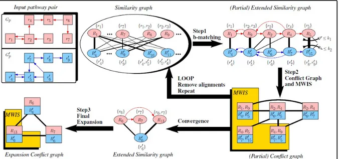
, respectively. These major steps are shown in Figure 2.1 on a metabolic pathway pair. The details are explained in the next subsections.
2.3.1. Constructing Bipartite Similarity Graph
In the first step, Cons(uRx) and Cons(uR0y) are created for every node uRx in G
k p and uR0 y in G 0 p k
where |Cons(uRx)| ≤ k1 and |Cons(uR0y)| ≤ k2. Let we have an edge-weighted bipartite graph where the first partition corresponds to the nodes of Gkp, the other partition corresponds to the nodes of G0pk and also, an edge between two nodes includes the homological score of these nodes. At this point, finding a subset of edges that provides the
Figure 2.1. CAMPways algorithm
degree constraints k1 and k2 and also, maximizes the total weight of the edges in that subset
is the major goal of the algorithm. In Figure 2.1, the thickness of the edges represents the weight of the edges such that the thickest edge corresponds to the highest score.
The major goal of the algorithm turns the problem into b-matching or degree con-strained subgraph problem that have been studied in the previous works [35] such that poly-nomial time solutions, network-flow algorithms and also, belief propagation methods have been suggested [36, 37]. Nevertheless, instead of using them, we prefer to use a simple greedy algorithm to provide the efficiency. The greedy algorithm selects the heaviest edge in the
bipartite graph considering the degree constraints k1 and k2 for both end points and the
output edge set. When there exists no edges that are appropriate for selecting due to edge weight and degree constraints k1 and k2, the algorithm stops and we have a bipartite graph
that consists of the selecting edges and nodes that are connected by these edges. Afterwards, we called the obtained bipartite graph as the similarity graph, S.
2.3.2. Conflict Graph Generation and Conflict Resolution
Let we assume that the bipartite similarity graph S is extended by the directed edges of Gk
p and G
0 p
k
due to a restriction such that if there exists an edge (uRx, uRy) in the graph Gkp, then the edge (uRx, uRy) is added to the similarity graph. Of course, same restriction is valid for the G0pk, as well. After the extension of the similarity graph, an undirected node-weighted conflict graph is created where the nodes of that graph corresponds to a set of four nodes that provides conserved edges in the similarity graph S. Actually, a node that corresponds to a 4 − tuple ≺ uRx, uRy, uR0x, uR0y is added to the conflict graph if and only if the following are satisfied:
1. Rx∩ Ry = ∅ and Rx0 ∩ R0y = ∅. 2. Either (uRx, uRy), (uR0x, uR0y) are in G k p, G 0 p k
respectively,or (uRy, uRx),(uR0y, uR0x) are in Gkp, G0pk respectively.
3. {uRx, uR0x}, {uRy, uR0y} are undirected edges in S.
For each node that corresponds to a 4-tuple in conflict graph is called as c4and a score is
assigned as a weight to every c4such that while the score is 1 if only the first part of the second
condition is satisfied, 2 is assigned as the score if all parts of the second condition is provided. At this point, it is possible to see that every node c4 of the conflict graph corresponds to
a pair of reaction subset mappings and provides at least one conserved edge in the output
alignment set. Furthermore, the weight of a c4 represents the conserved edge number that
is provided by that node. In figure 2.1, the exact conflict graph that is obtained from the partial similarity bipartite graph is showed. Whereas the 4 − tuple ≺ uR9, uR2, uR05, uR06 may denote a c4, it does not happen due to condition 1 such that the reaction subsets of R9
and R2 share the common reaction r2 in the partially extended similarity graph as shown in
figure 2.1. Also, when examining the weight of the c4s, it is possible to understand that the
weight are one according to the same figure.
Let the conflict nodes C1, C2 correspond to the 4 − tuples ≺ uRx, uRy, uR0x, uR0y and ≺ uRw, uRz, uR0w, uR0z , respectively. Moreover, let S1, S2 be the elements of {Rx, Ry}, {Rw, Rz} and S10, S 0 2 be the elements of {R 0 x, R 0 y}, {R 0 w, R 0
z}, respectively. For a c4 node Ci,
let MCi(u) denotes the neighbour of u in Ci from the opposite network. In this case, an edge is added between two c4 nodes if and only if at least one of the following satisfied:
1. ∃S1, S2 such that S1 6= S2 and S1∩ S2 6= ∅.
2. ∃S10, S20 such that S10 6= S0 2 and S 0 1∩ S 0 2 6= ∅.
3. ∃S1, S2 such that S1 = S2 and MC1(S1) 6= MC2(S2). 4. ∃S10, S20 such that S10 = S20 and MC1(S
0
1) 6= MC2(S
0 2).
Totally, these conditions indicate that there exists an edge between two c4s in the
conflict graph such that the conserved edges corresponding to these c4 nodes cannot coexist
in a legal alignment set. For instance, the edge is added between the c4 nodes corresponding
to the 4−tuples ≺ uR1, uR9, uR04, uR05 and ≺ uR2, uR4, uR06, uR07 in the conflict graph due to condition 1 such that the reaction subsets R9 and R2share a common reaction. Accordingly,
there is no legal alignment that consists of both these c4s due to shared reactions. On the
other side, the edge is added between the c4 nodes corresponding to the 4 − tuples ≺
uR4, uR5, uR07, uR015 and ≺ uR2, uR4, uR06, uR05 due to condition 3 such that whereas the reaction subset R4matches with the reaction subset R07 in one c4, in the other one, it matches
with the reaction R05 and matching between different reaction subsets is not allowed to be in the legal alignment set at the same time. In addition, these conditions and the construction of the conflict graph supports the following proposition:
Proposition 2.3.1. The maximum weight independent set (MWIS) of C provides an opti-mum solution to the constrained alignment problem.
Before the maximum weight independent set solution, we need some modifications to make our conflict graph model more useful in the framework. Firstly, in order to increase the quality of the alignment, we propose two weighting formulas for the conflict graph nodes. Let ws(e) be the weight of the edge e in the similarity graph S such that this weight indicates the
homological score between the reaction subsets corresponding to the end points of the edge e. The first weighting scheme is denoted by W1that equals to α x H(CI)+(1−α) x I(CI) where
CI corresponds to the conflict node that represents the 4 − tuple ≺ uRx, uRy, uR0x, uR0y and H(CI), I(CI) correspond to the following:
H(C1) = 1 2× (wS(uRx, uR0x) + wS(uRy, uRy0)) I(C1) = 1 2(k2+ 1) × X i,j∈{uRx,uRy},i6=j i0,j0∈{u R0x,uR0y},i 06=j0 w(i, j) + w(i0, j0)
In order to calculate I(C1), the total number of directed edges that are between Rx, Ry
and between R0x, R0y is normalized with the maximum number of possible directed edges in any conflict node c4. The parameter α is a balance parameter such that it balances the
rela-tionship between homological similarity score and topological similarity score. On the other
side, our second weighting scheme that is denoted by W2 does not check the conserved edge
number between the reaction subsets due to knowledge of providing at least one conserved
edge by each c4. Furthermore, depending on the evolutionary distances between the
alignments and one-to-few alignments is more meaningful. We use additional parameters a1, a2..., ak in second weighting scheme W2 in order to make a such differentiation such that
a1 + a2 + ... + ak = 1 and each ai corresponds to importance of one-to-i mappings in the
total alignment. Thus, for the node C1 =≺ uRx, uRy, uRx0, uR0y , W2 is calculated as a|Rx| x |Rx| + a|Ry| x |Ry| where |Rx| ≥ |R
0
x| and |Ry| ≥ |R0y|.
After the construction of the conflict graph, second important issue is solving that conflict graph which means solving the maximum weight independent set (MWIS) problem on the conflict graph and obtaining the maximum number of conserved edges. In gen-eral, the maximum weight independent set problem is in NP-Complete problem set [38]. In order to solve MWIS problem, several greedy heuristic algorithms have been proposed [39]. We implement and test the performance of all greedy heuristic algorithms and de-cide on GWMIN2 algorithm that gives best results for our algorithm. GWMIN2 algorithm, firstly, selects a node u in the conflict graph C such that the node u maximizes the score
of W(u)/P
v∈NC+(u)W(v) where N
+
c (u) denotes the node u and all neighbors of it. This
process goes on until there is no node in the conflict graph. Besides, the algorithm pro-vides a theoritical guarantee such that the weight of the output independent set is at least P
u∈VC[W(u)
2
/P
v∈NC+(u)W(v)] where Vcdenotes the vertex set of the conflict graph C.
De-pending on the results of our performance tests and the theoreticall guarantee of GWMIN2 algorithm, we prefer to use that algorithm to solve conflict graph.
Consequently, it is possible to see that we find a mapping set that consists of the edges in the bipartite similarity graph S based on the process of the Step 1 and also depending on the constraints k1, k2, our mapping set is limited. Obviously, extending the mapping set
increases the meaningful results. In order to extend the alignment set, firstly we restore all
homological edges and we remove the mapped nodes from Gk
p,G 0 p
k
after the steps 1 and 2 are over and afterwards, we repeat the steps 1 and 2. The loops go on until the conflict graph C produce empty set. For the sample input pathway pair in Figure 2.1, the loop iterates
only once such that after the step 1 and 2 works once, remaining extended similarity graph consists of the nodes R6, R7, R13, R60 and no conflict graph is produced by these nodes.
2.3.3. Final Alignment Expansion
Step 1 and Step 2 produce mappings based on the maximization of the conserved edge number and depending on the loops, it is possible to see that after the loops are over, the algorithm cannot produce more conserved edges anymore. But, still there may exist potential matchings that have high homological scores and these may be added the output alignment set. In order to provide such an extension, we restore all homological similarity
edges and remove all matched nodes from the graphs Gk
p,G 0 p
k
. At this point, we create a new conflict graph that is conceptually different from the conflict graph which is produced in Step 2, based on the remaining bipartite similarity graph S. The conflict graph is called expansion conflict graph and each node in that graph corresponds to a 2−tuple ≺ uRx, uR0x where {uRx, uR0x} is an edge in the remaining bipartite similarity graph S. An edge is added between two nodes in the expansion conflict graph if and only if the intersection of the reaction subsets which belong to the same pathway is not empty. The expansion conflict graph construction is shown in Figure 2.1. After the construction of the expansion conflict graph, GWMIN2 algorithm is used to solve conflicts on that graph as same as in Step 2 and finally, the output matching of GWMIN2 algorithm are added in the output alignment set.
2.4. Extension of Constrained Alignment Framework and CAMPways Algorithm
In this section, we extend the constrained alignment framework and CAMPways algo-rithm for one-to-one pairwise protein-protein interaction network alignment by making the necessary changes and additions in order to get reasonable and useful results. We give the problem definition for this problem and define major steps of CAPPI algorithm.
2.4.1. Problem Definition for PPI Network Alignment
Let simple undirected graphs G1(V1,E1) and G2(V2,E2) be the input PPI networks
where V1,V2 denote the sets of nodes corresponding to the proteins and E1,E2 denote the
sets of edges corresponding to the interactions, respectively. Moreover, let undirected edge-weighted bipartite graph S be the similarity graph where the partitions of S are V1,V2 and
each edge (u, u0) in S has a positive real weight w(u, u0). In many studies, the weight is a sequence similarity score w(u, u0) that is usually obtained by using BLAST between sequences of u and u0, where u ∈ V1 and u0 ∈ V2. BLAST bit score is the most preferred score that
is a log-scaled score and indicates biological relevance of a finding. But, when you compare the sequences of different species by using BLAST, you may not obtain all pairwise scores such that some pairwise scores are found as zero. So, the number of scored sequences which are taken as input may not be sufficient in some cases in order to get remarkable results.
According to Alada˘g and Erten [28], ”most of global network alignment algorithms can be
viewed to proceed in two phases. For each pair ui ∈ V1,vj ∈ V2, an estimate confidence score
is sought at an initial coarse-grained phase. The score represents the level of confidence that the match (ui, vj) is in the optimum alignment maximizing the global score. This is usually
followed by a fine-grained phase that consists of refining an initial global alignment based on the estimate scores attained in the previous phase”. Correspondingly, we prefer to use estimate confidence scores instead of BLAST bit scores and in this case, we obtain some advantages such as increase in the number of scored sequences and decrease in the running time. Thus, formally, the weight w(u, u0) of each edge (u, u0) is the estimate confidence score that is produced in SPINAL coarse-grained phase in our study.
Hereby, we need to give a definition for the legal alignment such that the definition is simpler than the problem definition of metabolic pathways within one-to-many alignment perspective. Because we focus on only one-to-one mappings, the connected subsets that are employed in the metabolic pathway alignment problem are not considered. Thus, in a simple
way, a legal alignment A occurs between G1 and G2 if for any matched pairs (u, u0) ∈ A
and (v, v0) ∈ A, u 6= v and u0 6= v0. This condition implies the uniqueness of the output
alignment such that each node in G1 can match with only one node in G2 and vice versa.
Afterwards, the important point is the quality of the alignment. As it is mentioned in the previous sections, the quality of the alignment corresponds to the similarity measure in terms of both homological and topological similarities. Because the subject is PPI networks, while we use estimate confidence score that is mentioned before as homological similarity score, we give the definition of the topological similarity score as in the problem definition of metabolic pathways in terms of conserved edge number. There exists a conserved edge for any matched pairs (u, u0), (v, v0) where u, v in V1 and u0, v0 in V2, if there is an undirected edge (u, v) in
G1 and an undirected edge (u0, v0) in G2. Consequently, in a similar way, the major goal of
the PPI network alignment is maximization of homological and topological scores.
2.4.2. CAPPI Algorithm
As it is mentioned before, because the major goal consists of both homological and topological similarities, we propose an algorithm that balances these scores with a parame-ter. While high-valued parameters handle the problem within conserved edge maximization, low-valued parameters give alignment results based on better biological meaning. As both versions are explained in same sections, in general, CAPPI algorithm consists of four main steps assuming G1, G2, S, the constants k1, k2, α, f, b, i and the homological similarity score
(estimate confidence score) w(u, u0) is given where u and u0 are any nodes in G1 and G2,
respectively. The details are given in the next sections.
2.4.3. Finding Maximum Weight Bipartite Matching
Because the general framework is based on the conserved edge maximization, while obtaining the conserved edges, some maximum homologically weighted pairs may be missed
if they don’t provide any conserved edge or they may not be selected due to conflict status. In order to handle this case, we employ a maximum weight bipartite matching (MWBM) on the bipartite similarity graph S. Let b be a parameter that is used to define the number of matchings that are taken from the alignment set of maximum weight bipartite matching such that the first b maximum weighted pairs are taken from the alignment set of MWBM and added to the actual alignment output set of CAPPI algorithm. Afterwards, the nodes
and edges that are in the selected pairs are removed from G1, G2 and S. Next steps of
CAP P I algorithm go on the remaining graphs. These processes are based on the value of the constant f such that if f equals to one, then finding maximum weight bipartite matching step is employed but when the value of f equals to zero, this step is not performed and the original graphs G1, G2 and S are used in the next sections.
2.4.4. Constructing Reduced Bipartite Similarity Graph
Initially, we assume that we have a bipartite similarity graph such that the first
parti-tion nodes correspond to the nodes of G1 and second one includes the nodes correspond to
the nodes of G2. The edges that are between two partitions have estimate confidence scores.
But we change these scores according to the goal of the algorithm. When the goal is finding more conserved edges, high-valued α parameter is used. However when the goal focuses on biological meaning, low-valued α parameter is preferred. Thus, the score is based on both homological and topological score and the score equals to α× min(|Eu|, |Eu0|) + (1 − α)
×w(u, u0) for any node u in G
1 and any node u0 in G2. In this formula, while w(u, u0) denotes
the estimate confidence score between the nodes u, u0, |Eu| and |Eu0| denotes the number of
edges of u and u0 in the original graphs G1 and G2, respectively. We take the minimum
number of edges and it is possible to see that the minimum number of edges indicates the possible conserved edge number for a node pair and if all edges are legal in the conflict graph, then the pair gives maximum min(|Eu|, |Eu0|) conserved edges. Also, it is possible to
In order to explain this step, we need to give the constrained definition for this problem depending on the constrained alignment framework. In a similar way, Cons(u) denotes the
constraints set of u in G1 and includes the possible nodes that the node u can mapped to.
Of course, the same definition can be used for the nodes of G2. The same symmetry that
is mentioned in the constrained framework can be used for this problem as well such that u0 ∈ Cons(u) if and only if u ∈ Cons(u0) depending on |Cons(u)| ≤ k
1 and |Cons(u0)| ≤ k2
for any nodes u in G1 and u0 in G2 and fixed constants k1, k2.
This step reduces the original bipartite similarity graph based on these constraints such that all constraints Cons(u), Cons(u0) are created for every node u of G1 and u0 of G2 where
|Cons(u)| ≤ k1 and |Cons(u0)| ≤ k2. In the fact, the problem is to find an edge subset
that maximizes the sum of edge weights by providing the constraints k1 and k2. In order to
solve this problem, we use the same greedy algorithm that is used for metabolic pathways alignment in CAMPways algorithm and obtain reduced bipartite similarity graph.
2.4.5. Conflict Graph Generation and Conflict Resolution
In general concept, conflict graph generation and conflict resolution is same as CAM-Pways algorithm. But, in order to get better results we make some changes in this step.
Let the reduced bipartite similarity graph be extended with the edges of G1 and G2 and
afterwards, an undirected node-weighted conflict graph is created such that each node in the conflict graph corresponds a 4-tuple ≺ u, u0, v, v0 and is denoted as c4, as well. In detail,
the node that corresponds to 4-tuple ≺ u, u0, v, v0 is added to the conflict graph if and only if the following are satisfied:
1. u 6= v and u0 6= v0.
2. The undirected edge (u, v) is in G1 and the undirected edge (u0, v0) is in G2.
3. {u, u0} and {v, v0} are undirected edges in S.
In the conflict graph, a weight is assigned to each node such that the weight of c4 that
corresponds to the 4-tuple ≺ u, u0, v, v0 equals to the following:
W (c4) = ( 1 2× (w(u, u 0 ) + w(v, v0))) |e|
where |e| denotes the number of possible conserved edges such that it is possible to see that each c4 denotes one conserved edge and it is important to check that if that conflict node
is selected in resolution phase, what is the contribution of that node to the conserved edge number in the output alignment. Thus, the number of possible conserved edges |ep| that are
contribution of the conflict node to the output alignment is added to one and |e| = 1 + |ep|.
It is clear that whereas in the first loop, that score is only one, but in the next loops the score is changed due to output alignment set that is provided by conflict resolution.
In this step, the second important issue is to add edges between the conflict nodes. Let C1, C2 be two conflict nodes corresponding to 4-tuples ≺ u, u0, v, v0 and ≺ w, w0, z, z0 ,
re-spectively. Let S1, S2and S10, S 0
2 be the unions of the nodes {u, v},{w, z} and {u
0, v0},{w0, z0},
respectively. Furthermore, for a c4 node Ci, let MCi(u) denotes the neighbor of u in Ci from the opposite network. In this case, the condition of adding an edge is same as in CAMPways algorithm. Thus, the conditions are not given again in order to prevent tautology.
After the construction of the conflict graph, we need to solve the conflicts in an optimum way. Similarly, we use GWMIN2 algorithm that is used in CAMPways algorithm within same definitions. However, because this algorithm is heuristic, we extend it with some modifications. Without loss of generality, we use the swap idea in the algorithm such that the impact of that idea is negligible on the running time and it helps to increase the size of the alignment set that is provided by GWMIN2. The swap idea have been used in both the alignment problems and bioinformatics studies in order to get better results [40, 41]. At this point, we use a simple swap process such that after GWMIN2 is completed, we try to swap the nodes that are in the alignment set with the nodes in the conflict graph that are legal for being in that set. The swap iteration starts from the first node in the alignment set, removes this node from the set and finds the legal nodes that are not conflict with the nodes in the remaining alignment set. Afterwards it compares the score of the node in the alignment set with the total score of legal nodes. If the total score is greater than the score of the node in the alignment set, then it swaps these nodes. The iteration goes on until all nodes are checked in the alignment set.
Obviously, the alignment set that is provided by GWMIN2 includes the node pairs based on the reduced bipartite similarity graph. Still, for the original bipartite similarity graph, there may exist some matching that are created conflict graphs. Thus, in order to extend the alignment set and obtain possible matching based on the conflict graphs, we restore the bipartite similarity graph and remove the nodes that are in the alignment set of GWMIN2 from the similarity graph. Afterwards, we repeat step 2 and 3 until the bipartite similarity graph does not produce any conflict graph. The constant i defines the number of such iterations. When the goal is maximization of the conserved edges, then the value of constant i is higher and in that time, we observe that the homological score decreases depending on the natural concept of the framework such that when the iterations are employed, while the conserved edge number increases, the biological meaning decreases. Thus when the better results in terms of biological meaning are aimed, then second and
third steps are employed only once.
2.4.6. Final Alignment Expansion
Final Alignment Expansion parts of CAMPways and CAPPI are completely different. While CAMPways try to find conflicts due to 2-tuples, CAPPI uses maximum weight bipar-tite matching such as in step 1 of CAPPI algorithm. However, depending on the constant f , maximum weight bipartite matching algorithm uses different values. As it is mentioned before, when the constant f equals to zero, the algorithm aims to find more conserved edges. Thus, when the iterations are over, the edge weights of remaining bipartite similarity graph are changed depending on the aim. For each pair of the remaining bipartite similarity graph, the conserved edge contribution number is calculated such as in conflict graph generation step. The possible conserved edge number that is provided by the pair if it is selected for being in the alignment graph is assigned as a weight to the considered edge. Afterwards, the maximum weight bipartite matching algorithm is used on the remaining bipartite similarity graph within these scores. The alignment set that is produced by that algorithm is added to the actual alignment set. However, when the constant f equals to one, the goal is maxi-mization of the biological meaning. Thus, the edge weights of remaining bipartite graph are selected as estimate confidence scores and similarly, the alignment set that is produced by that algorithm is added to the actual alignment set.
3.
COMPLEXITY ANALYSIS
3.1. NP-Hardness Proof of Constrained Alignment Problem
Proposition 3.1.1. The constrained alignment problem where k = k1 = 1 and k2 = 3 is
NP-Complete.
Proof. As it is defined previously, the problem refers to one-to-one alignment between the nodes of Gp and G0p in case k equals to one. In addition, the constraints that express k1 = 1
and k2 = 3 mean that each node of Gp can be aligned with one node of G0p and on the other
side, each node of G0p can be aligned with one of at most 3 nodes of Gp.
Because of a problem x in NP-Complete is also in both NP and NP-Hard, we need to handle the proof from both directions. So, under these considerations, according to general proof strategy, we first need to show that the problem is in NP by giving an efficient certifi-cation. Hereby, the set of mappings between the nodes of Gp and G0p gives the certification
and shows that the problem is in NP which means the problem is a decision problem within yes or no answers that yes answers can be proved in polynomial time. For this problem, yes answers correspond to checking whether the provided alignment is legal or not within all these considerations and whether is it giving at least a fixed number f of conserved edges or not. In order to show NP-Hardness of the problem, we use reduction from Monotone 1in3SAT that is a restricted version of 3SAT such that while every clause has exactly three literals and exactly one of them is true, no negations in the clauses are allowed. Whereas the reduction is based on the undirected graphs, it can be adapted to directed graphs as well. In order to generalize the reduction for directed graphs, we make each edge of Gp and
Figure 3.1. NP-Hardness Proof Graph
According to the reduction idea, firstly, we need to create graphs that represent the variables and clauses. Thus, we start by creating Gp. A clause cluster is created for each
clause (xi ∨ xj ∨ xk) in a given Monotone 1in3SAT instance φ where the nodes ci, cj, ck of
the cluster correspond to xi, xj, xk in the clause. Furthermore, a variable cluster is created
for each variable xt in φ where the nodes vt, ¯vt correspond to xt, ¯xt. Each node ci in a
clause cluster is connected to three nodes vi, ¯vj, ¯vk in variable clusters. Thus, Gp becomes
a bipartite graph where one partition consists of clause clusters and the other partition consists of variable clusters. Creating G0p is simpler than Gp such that the nodes are created
corresponding to clause and variable clusters of Gp. The edges are added between all possible
node pairs and a complete graph is obtained. Eventually, in order to represent the similarity edges, we add an edge between a node of G0p and its corresponding clusters in Gp. The figure
3.1 illustrates the graph definitions.
Hereby, our claim is that there exists a valid satisfying Monotone 1in3SAT assignment of variables in φ if and only if the global alignment score is at least f = 3|C| such that |C| refers to the number of clauses in φ. According to graph definitions and Figure 3.1,
![Figure 1.1. A metabolic pathway (taken from [1])](https://thumb-eu.123doks.com/thumbv2/9libnet/4328150.71131/17.918.131.822.197.423/figure-a-metabolic-pathway-taken-from.webp)
![Figure 1.2. A protein interaction network (taken from [2])](https://thumb-eu.123doks.com/thumbv2/9libnet/4328150.71131/20.918.169.756.182.503/figure-protein-interaction-network-taken.webp)