Comparison of simple sum and Divisia monetary aggregates using panel data analysis

ĐSTANBUL BĐLGĐ UNIVERSITY

INSTITUTE OF SOCIAL SCIENCES

COMPARISON OF SIMPLE SUM AND DIVISIA

MONETARY AGGREGATES USING PANEL DATA

ANALYSIS

Seda Uzun

ĐSTANBUL BĐLGĐ UNIVERSITY

INSTITUTE OF SOCIAL SCIENCES

COMPARISON OF SIMPLE SUM AND DIVISIA

MONETARY AGGREGATES USING PANEL DATA

ANALYSIS

Seda Uzun

In Partial Fulfilment of

the Requirements for the Degree of Master of Science in Economics

May 2010

Approved by:

I Abstract

It is well documented that financial innovation has led to poor performance of simple sum method of monetary aggregation destabilizing the historical relationship between monetary aggregates and ultimate target variables like rate of growth and rate of unemployment during the liberalization period of 1980s. This thesis tries to emphasize the superiority of an alternative method of aggregation over the simple sum method, namely Divisia monetary aggregates, taking advantage of two testing methodologies, one of which is the system estimation (Seemingly Unrelated Regression (SUR)) using time series data and the other is the panel data analysis for United States, United Kingdom, Euro Area and Japan for the period between 1980Q1 and 1993Q3. After estimating the parameters of the system through SUR method, I have proceeded with the panel procedure and investigated the order of stationarity of the panel data set through several panel unit root tests and performed advanced panel cointegration tests to check the existence of a long run link between the Divisia monetary aggregates and income and interest rates in a simple Keynesian money demand function. Findings revealed that there exists a long run link between Divisia monetary aggregates, income (measured by real GDP) and interest rates and the relationship between these three variables is relatively robust when compared to the link between simple sum monetary aggregates, income and interest rates.

II To my beautiful aunt, Hülya Keskinel whom I always feel her hands on my shoulder and always looks at me through the stars.

III Acknowledgements

I wish to thank to my thesis supervisor, Assistant Professor Sadullah Çelik, for his guidance and invaluable contribution. He not only encouraged me to study on this thesis topic, but also helped me improve my ideas regarding this topic. I really appreciate that he shared his time, sources and previous and on-going studies with me.

I am also grateful to Mr. Kenjiro Hirayama and Mr. Livio Stracca for their efforts during the process of data collection. They provided me the relevant data and hence accelerated my thesis-writing process.

I also would like to give special thanks to a special person, Berk Saraç for his endless support not only through his special advices but also through his love.

Finally, and the most importantly, I want to thank my family, especially my mother Özgül Uzun since she helped me use my time effectively and provided me with a suitable working environment. I also would like to thank my father, Tayfun Uzun for his researches on my thesis and the relevant Turkish sources that he found. My brother, Emre Uzun and my uncle, Ali Keskinel helped me in technical and design-related issues. My aunt, Derya Ramos also did her best in order for me to focus only on my thesis. I also thank my grandmother, Ayten Levent for her positive energy.

IV Table of Contents

1. Monetary Aggregation ... 5

1.1. The Origins of Monetary Aggregation ... 8

1.2. Theoretical Framework of Monetary Aggregation ... 11

1.2.1. Consumer Choice Problem ... 12

1.2.2. Weak Separability Assumption and Aggregator Functions ... 16

1.3. Statistical Index Numbers ... 19

1.4. Barnett’s Contribution... 22

2. The Formulation of New Monetary Aggregates ... 25

2.1. Divisia Monetary Aggregates ... 26

2.2. Currency Equivalent Index ... 28

3. Historical Performance of Monetary Aggregates in Developed Countries ... 29

3. 1. United States: ... 30

3.2. United Kingdom:... 32

3.3. Euro Area: ... 34

3.4. Japan... 36

4. Econometric Methodology and Empirical Results for Developed Countries ... 38

4.1. Econometric Methodology ... 38

4.1.1. Seemingly Unrelated Regression (SUR) Analysis... 39

4.1.2. Panel Unit Root Tests ... 40

4.1.2.1. Levin, Lin and Chu (2002) Test (LLC Test) ... 41

V

4.1.2.3. Peseran (2007) CIPS Test ... 42

4.1.3. Panel Cointegration Tests ... 43

4.1.3.1. Pedroni (1999, 2004) Test ... 43

4.1.3.2. Westerlund (2007) ECM Panel Cointegration Tests ... 44

4.1.3.3. Westerlund and Edgerton (2007) Panel Cointegration Tests ... 44

4.1.4. Panel Fully Modified OLS Estimation... 45

4.2. Empirical Results ... 46

5. Conclusion ... 67

Appendix: The Data ... 70

VI List of Tables

Table 1: Two-step GLS - Dependent Variable SS ... 49

Table 2: Two-step GLS - Dependent Variable DIV ... 51

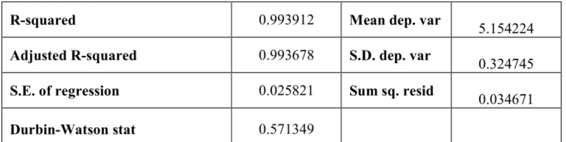
Table 3: Iterative GLS - Dependent Variable SS ... 53

Table 4: Iterative GLS - Dependent Variable DIV ... 55

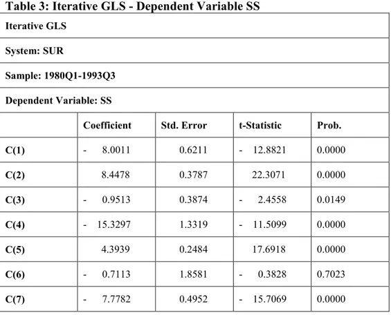
Table 5: Residual Correlation Matrix – SS ... 57

Table 6: Residual Correlation Matrix – DIV ... 58

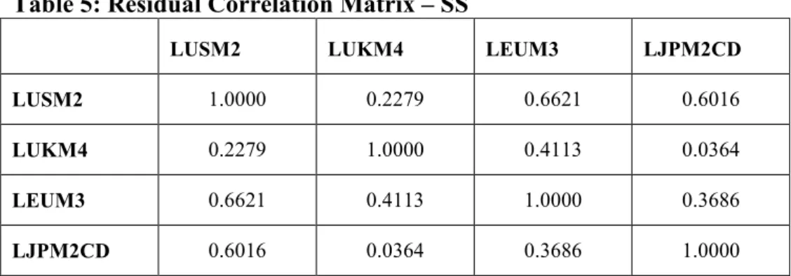
Table 7: Wald Coefficient Test - SS ... 59

Table 8: Wald Coefficient Test – DIV ... 59

Table 9: Panel Unit Root Tests in Levels ... 61

Table 10: 1st Generation Panel Cointegration Test: Dependent Variable DIV ... 62

Table 11: 1st Generation Panel Cointegration Test: Dependent Variable SS ... 63

Table 12: 2nd Generation Panel Cointegration Tests: Dependent Variable DIV ... 64

Table 13: 2nd Generation Panel Cointegration Tests: Dependent Variable SS ... 65

VII List of Figures

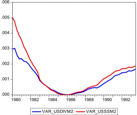
Fig. 1. Variance of Simple Sum and Divisia M2 in U.S ... 31

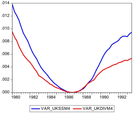
Fig. 2. Variance of Simple Sum and Divisia M4 in the U.K ... 33

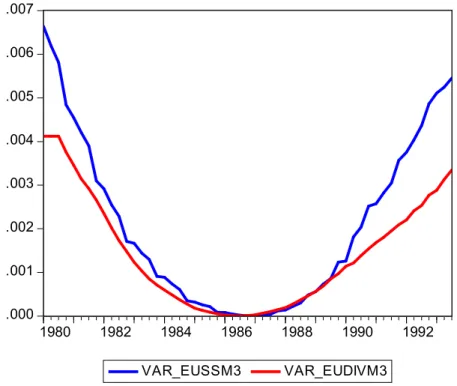
Fig. 3. Variance of Simple Sum and Divisia M3 for Euro Area ... 35

1

Introduction

It is highly difficult to deny the direct relationship between the money supply and key macroeconomic variables such as output and inflation. In this context, the issue of monetary aggregates has been studied in the literature and the possible casual link between money and real variables has been examined by empirical studies supported by the theoretical framework. From the monetarist perspective, money affects inflation and does not affect output and unemployment in the long run even if the short term effect of money on these real variables is considerable. Monetarists recommended a fixed target growth rate for base money in order to achieve price stability on which many central banks base their monetary policy. Price stability is important because a rising price level-inflation imposes substantial economic costs on society. Some of these costs are increased uncertainty about the outcome of business decisions and profitability, adverse effects on the cost of capital caused by the interaction of inflation with the tax system and reduced effectiveness of the price and market systems. Achieving price stability and hence obtaining the desired long run results of this policy through a fixed target rate for base money requires two conditions: one is the necessity for a stable money demand so that the impact of monetary policy will be predictable and the other one is the need for a stable money multiplier meaning that the changes in broad money supply might be forecasted by the changes in monetary base. The stability of money demand functions is important due to the fact that it reflects the predictive ability for

2 future economic activity. Therefore, any uncertainty affecting the choice of a money supply indicator for predicting future economic performance of a country also affects the estimation of money demand models.

The general view of the early 1970s was that there exist a considerable linkage between broad monetary aggregates and the real variables such as output and unemployment. Therefore, major industrial countries adopted some form of monetary growth target as a guide or intermediate objective of monetary policy. Friedman (1982a) and Dennis (1982), in their studies, mentioned about the major reasons behind the switch to monetary targeting. These reasons were the acceleration of inflation in the early 1970s and hence the difficulty in interest rate targeting, the expectation that small and open economies could conduct their own monetary policy independently and finally the dissatisfaction with the fine-tuning policies which rely on the fact that money supply should be demand-determined. In this respect, in 1975, the Federal Reserve began to report annual target growth ranges for M1, M2, M3 and the bank credit and after 1977, the target was defined as “ maintain long run growth of monetary and credit aggregates… so as to promote effectively the goals of maximum employment, stable prices and moderate long term interest rates”. Also the Federal Open Market Committee under the Chairman Paul Volcker adopted a policy based on monitoring non-borrowed reserves so as to control the growth of M1 and M2 and thereby reduce inflation. However, after the second oil crisis of 1979, monetary targeting procedures became subjects of considerable debate not only in the United States but also in other countries and the close

3 relationship between the monetary aggregates and the targeted real variables was questioned due to the deregulation of financial markets, the financial innovation, the competition between financial intermediaries, the rapid development of new information and the liberalization attempts in terms of free capital flows and the introduction of flexible exchange rates. These developments seen in the early 1980s certainly affected the definition of money, the money supply process and the stability of demand for money. For instance, in 1982, the Federal Reserve Board argued that it would be convenient to pay less attention to M1 and focus on broader monetary aggregates. Moreover, Hendry (1995) argued that the instability in M1 demand forced Bank of Canada (BOC) to abandon M1 as a target variable. In the early 1980s, the United Kingdom also gave less weight to its sterling M3 target.

Not only the above mentioned developments in the early 1980s resulted in the instability of the demand for money, but also the aggregation method used for the components of monetary aggregates supplied by many central banks has caused induced instability of money demand and supply conditions. The aggregation method mentioned here is simply the simple sum method. This procedure has been criticized due to the fact that this method of aggregation weighs each component equally. In other words, this procedure treats all included assets equally in terms of “moneyness” (“money substitutes”, “near money”, “secondary liquidity” etc.) and the excluded variables as the ones providing no monetary services. This fact paves the way for new monetary aggregates one of which is the famous

4 Divisia monetary aggregates which allow for a weighted aggregate of components in order to measure the flow of monetary services.

In this thesis, I basically aim to show the performance of Divisia monetary aggregates calculated for the advanced countries (the Unites States, the United Kingdom, Euro Area and Japan) over their simple sum counterparts covering a period between 1980 Q1 and 1993 Q3. Within this framework, I try to answer the following two questions:

• Is there any evidence that Divisia monetary aggregates of the relevant countries perform well when compared to their simple sum counterparts?

• Does there exist a significant long run link between the Divisia monetary aggregates, income and interest rates in a simple Keynesian money demand function?

In the first chapter of this thesis, I will argue for the concept of monetary aggregation and the theoretical background of the monetary aggregation. The second chapter mentions about the formulation of new monetary aggregates including Divisia monetary aggregates and currency equivalent indexes. The third chapter touches upon the historical performance of monetary aggregates in the relevant developed countries while the forth chapter explains the methodology of the econometric tests and methods (SUR method (using time series data) and unit root and cointegration tests, and Fully Modified Ordinary Least Squares estimation (using panel data)) and reveals the empirical findings regarding the results of these tests

5 considering the previous studies on the comparison of simple sum and Divisia monetary aggregates. The final chapter is devoted to the conclusion of this thesis.

1. Monetary Aggregation

The monetary assets held by consumers, firms and other economic decision makers play a significant role in macroeconomics. These economic units hold these aggregate quantities for the purposes of transaction, speculation and contingencies. Monetary aggregates published by central banks in aggregate forms like M1, M2, M3 or L are generally the sums of the amounts of monetary assets in dollar or in other currencies. The content of these aggregates vary from one country to another. In this context, it would be convenient to discuss the monetary aggregates of United States (U.S), United Kingdom (U.K), Euro Area (E.A) and Japan, which are constructed by summation procedure:

United States:

M1 = Currency and Travellers’ Checks + Demand Deposits Held by Consumers + Demand Deposits Held by Businesses + Other Checkable Deposits + Super NOW Accounts Held at Commercial Banks + Super NOW Accounts Held at Thrifts

M2 = M1 + Money Market Mutual Fund Shares + Money Market Deposit Accounts at Commercial Banks + Money Market Deposit Accounts at Thrifts + Savings Deposits at Commercial Banks + Savings Deposits at Savings and Loans (S&Ls) + Savings Deposits at Mutual Savings Banks

6 (MSBs) + Savings Deposits at Credit Unions + Small-Time Deposits and Retail RPs at Commercial Banks + Small Time Deposits at S&Ls and MSBs and Retail RPs at Thrifts + Small Time Deposits at Credit Unions

M3 = M2 + Large Time Deposits at Commercial Banks + Large Time Deposits at Thrifts + Institutional Money Market Funds + RPs at Commercial Banks and Thrifts + Eurodollars

L = M3 + Savings Bonds + Short-term Treasury Securities + Bankers’ Acceptances + Commercial Paper.

United Kingdom:

M2 = notes and coins held by the U.K non-bank and non-building societies of private sector + the sterling retail deposits with the U.K banks and building societies + the cash component of M4.

M4 = notes and coin held by the U.K private sector other than monetary financial institutions + sterling deposits at Monetary Financial Institutions (MFIs) in the U.K + certificates of deposit and other paper issued by MFIs of not more than 5 years original maturity.

Japan:

M2 = cash currency in circulation plus deposits deposited at Domestic Banks etc.

M2 +CDs1 = M1 + private and public deposits less demand deposits with financial institutions surveyed + certificates of deposit including those of

1

M2+CDs is also described as the sum of quasi-money (time deposits held at Bank of Japan, All Banks, Shinkin Banks, the Norinchukin Bank and the Shoko Chukin Bank) and certificates of deposit (CDs), which are introduced in 1979 and whose interest rates are market determined.

7 private corporations, individuals and the public with the financial institutions surveyed.

M3 = Cash Currency in Circulation + Deposits deposited at Depository Institutions.

L = M3 + pecuniary trusts + investment trusts + bank debentures + straight bonds issued by banks + commercial paper issued by financial institutions + government bonds + foreign bonds.

Euro Area:

M1 = Currency in circulation + overnight deposits

M2 = M1 + Deposits with an agreed maturity up to 2 years + Deposits redeemable at a period of notice up to 3 months

M3= M2 + Repurchase agreements + Money market fund (MMF) shares/units + Debt securities up to 2 years

The monetary quantity aggregates supplied by these central banks are the simple unweighted sums of the component quantities. These aggregates are constructed by the summation procedure in which a weight of unity is assigned to each monetary asset and the owners of these assets regard these assets as perfect substitutes. Fisher and Fleissig (1997) argue that the simple sum aggregation procedure might be useful for policymakers under the condition that interest rates do not fluctuate very much. However, significant fluctuations in interest rates reveal some doubts in terms of the appropriateness of simple sum aggregation method. Besides that, economic agents hold a portfolio of monetary assets, which have different opportunity costs. Therefore, it would be inconvenient to consider that the simple sum

8 aggregation procedure captures the true dynamics of the asset demand theory.

As the number of financial assets treated as money increased substantially, the idea of treating these assets as perfect substitutes would be inconvenient. Since some financial assets have more “moneyness” than others, they deserve larger weights. In this context, it would be useful to demonstrate the first attempts at constructing an alternative to simple sum aggregate.

1.1. The Origins of Monetary Aggregation

Economic deals with two distinct aggregation problems, one of which is aggregation across heterogeneous agents and the other is aggregation of the various goods purchased by a single agent. This thesis focuses on the latter, examining the aggregation of monetary assets held by a single representative agent.

In the literature, there have been many studies discussing the microfoundations of money2. However, prior to Barnett (1978, 1980, 1981); Hutt (1963), Chetty (1969), and Friedman and Schwarz (1970) had applied either microeconomic aggregation theory or index number methods to monetary assets.

Hutt (1963) suggested the index known as the currency equivalent (CE) index of which the theoretical framework and the formulation developed by Rotemberg et. al (1995). He also explains two forms of money which are pure money and hybrid money and his aggregation consists of the

2

Among others, see Pesek and Saving (1967), Samuelson (1968), Niehans (1978) and Fama (1980).

9 combination of these two units so as to provide a future flow of monetary services. He argues that money should produce monetary services and attributes the difference between money and other assets to the value of money influenced by the demand of the monetary services provided by these monetary assets. However, his study actually lacks robust empirical support and is not based on a sound theoretical framework.

As for the study by Chetty (1969), he extended the portfolio of the monetary aggregates meaning that he added savings-type deposits to currency and demand deposits and estimated the substitutability between non-medium of exchange assets and the pure medium-of-exchange assets. For instance, using time series data for the United States covering a period between 1945 and 1966, Chetty finds that time deposits and savings and loan shares are good substitutes for money. He also defines an adjusted money stock based on the estimates obtained from the degree of substitution between monetary assets. One of the problems regarding Chetty’s approach is that the parametric tests used in his study are sensitive to specification errors.

The idea that the aggregation methods should keep the information contained in the elasticities of substitution and should not make strong a priori assumptions regarding these elasticities causes Friedman and Schwarz (1970) to deal with the problems regarding the proper definition of money. First of all, they form four monetary aggregates (currency, currency, demand deposits, time deposits, mutual savings bank deposits, savings and

10 loan shares3) through simple sum procedure. After constructing these four aggregates by simple summation of monetary asset, they offer a definition for the quantity of money as the weighted sum of the aggregate value of all assets and in the procedure they follow, all the weights are either zero or unity. Furthermore, a weight of unity is attached to assets having the largest quantity of "moneyness" per dollar of aggregate value. Actually, the major problem with this procedure is not only the way of assigning weights but also the potential instability in the weights assigned to individual assets.

The assessments made by the authors above mentioned could not touch upon the fact that even weighted aggregates might produce perfect substitutability unless the aggregation procedure is non-linear (Barnett et al. 1992). Nonetheless, monetary authorities have widely used simple sum monetary aggregates due to their availability. Goldfeld (1976) also mentioned about the poor performance of money demand functions employing simple sum aggregates. Since the common problem with forming weighted monetary aggregates and employing appropriate definitions of monetary aggregates for money demand functions was the lack of a robust theoretical background, Barnett (1978) started to focus on the microeconomic foundations of the monetary aggregation4 and built the theoretical framework of the new monetary aggregates. Before proceeding with the formulation of the new monetary aggregates, it would be better to consider the theoretical framework of these new monetary aggregates.

3

Friedman and Schwarz (1970) constructed 4 aggregates, one of which is the sum of the first two assets and the others are formed by adding one more asset to the added sums so as to reach the remaining three aggregates.

4

Microeconomic foundations of monetary aggregations can be illustrated in models of profit maximizing firms and financial intermediaries (Barnett, 1987).

11 1.2. Theoretical Framework of Monetary Aggregation

Microeconomic theory is necessary for monetary aggregation in order to express various monetary aggregates as a single aggregate. The general conditions which are sufficient for the aggregation of a group of economic variables are listed by Anderson et. al. (1997a). These conditions include: 1. The existence of a theoretical aggregator function defined over a group of variables (in other words, the existence of a sub-function that can be factored from the economic agent's decision problem);

2. Efficient allocation of resources over the group of variables; 3. No quantity rationing within the group variables;

4. Given that the underlying data have been aggregated previously across consumers, the existence of a representative agent.

These conditions permit the theoretical aggregation of a group of variables. However, these conditions do not allow the nature of the aggregates to be analyzed with the microeconomic theory. Anderson et. al (1997a) also specify some conditions in order to present strong linkages between monetary aggregation and microeconomic theory by focusing on the aggregation of monetary assets held by a representative consumer since assuming the existence of a representative agent is one of the methods of developing aggregate demand functions depending upon the microeconomic decision. These specific conditions include:

1. The weak separability assumption which implies the existence of a theoretical aggregator function defined over current period monetary assets;

12 2. The utility maximization which leads to the efficient allocation of resources over the weakly separable group;

3. Disregarding the quantity rationing.

In this context, the theoretical framework of monetary aggregation is based on solving the intertemporal decision problem of the representative consumer using weak separability assumption and a theoretical aggregator function which will be explained in the following sections:

1.2.1. Consumer Choice Problem

The existence of a representative consumer is important in developing aggregate demand functions, which are consistent with microeconomic decision rules. Besides that, it has been common practice in the literature to use a representative consumer while solving for optimal maximization5. This representative consumer faces the problem of maximizing its utility subject to a budget constraint and the equilibrium level of price and quantity is reached through first order conditions.

Monetary assets have taken place in utility functions since Walras (1954). Arrow and Hahn (1971) argue that given the positive value of money in general equilibrium, there exists a derived utility function including money6. Therefore, any model that does not contain money in the utility function but creates a motive for holding money in equilibrium is tantamount to a model

5

The stochastic method of aggregation does not employ a representative agent. Among others, some examples are Theil (1971), Barnett (1979, 1981) and Selvanathan (1991).

6

Fisher (1979) derives a production function that contains money balances. Feenstra (1986) introduces specific utility functions implied by several popular models of money demand. Duffie (1990) presents a review of general-equilibrium models in which money has positive value.

13 that includes money in the utility function. In this context, the generality in modelling does not disappear depending upon adding money component to the utility function.

The consumer’s choice problem starts with the assumption that the representative consumer maximizes intertemporal utility over a finite planning horizon of T periods7. The consumer’s intertemporal utility function in any period, t, is

U (mt, mt+1,..., mt+T; zt, zt+1,…, zt+T; lt, lt+1,…, lt+T; At+T),

where, for all s contained in {t, t+1,….,t+T}, ms is a vector of real stocks of

n monetary assets, zs is a vector of quantities of h non-monetary goods and

services, ls is the desired number of hours of leisure, and At+T is the real

stock of a benchmark financial asset, held only in the final period, at date t+T.

The representative consumer reoptimizes in each period, choosing the values of (mt, mt+1,…, mt+T; zt, zt+1,…, zt+T; lt, lt+1,…, lt+T; At+T) that

maximize the intertemporal utility function subject to a set of T+1 multiperiod budget constraints. This set of multiperiod budget constraints for s found in {t, t+1,….,t+T} is:

[

] [

]

∑

∑

Where p*s is a true cost of living index, ps is a vector of prices for the h

non-monetary goods and services, rs is a vector of nominal yields on the n

monetary assets, Rs is the nominal yield on the benchmark asset, ws is the

7

14 wage rate, As is the real quantity of a benchmark asset that is included in the

utility function only in the final period, t+T and Ls is the number of hours of

labor supply.

The consumer has leisure time, ls, during each period as, ls = H - Ls where H

denotes the total number of hours in a period. In the above representation, the real value of assets carried over from the previous planning period is

, 1 , 1 1 1 1 (1 ) (1 ) n i t i t t t i r − m − r − A − = + + +

∑

and the real value of the consumer’s provisions for the following planning periods is , , 1 (1 ) (1 ) n i t T i t T t T t T i r + m + R + A + = + + +

∑

The model also assumes that:

1. There exists a true cost-of-living index, p*s, as in Barnett (1987).

2. The utility function, U(.), contains all the services provided to the representative consumer by monetary assets, except for the intertemporal transfer of wealth.

3. Each period’s budget constraint includes the benchmark asset, As.

However, only the final period utility function contains it. The reason is that the benchmark asset is used to transfer wealth from one period to another during all periods, except the final period. The consumer stores all wealth in the form of the benchmark asset and transfers it to the next period until the final period. In this sense, the benchmark asset provides no monetary services to the consumer until the final period.

15 Before proceeding with the consumer’s choice problem, it is possible to simplify notation. Assume that the vector mt= (m1t,…,mnt) includes all

current-period monetary assets, and the vector xt= (mt+1,..,mt+T; zt, zt+1,…,

zt+T; lt, lt+1,…, lt+T; At+T) contains all other decision variables in the utility

function. Moreover, assume that the vectors m*t= (m*1t,…,m*nt) and x*t=

(m*t+1,…,m*t+T; z*t, z*t+1,..., z*t+T; l*t, l*t+1,…,l*t+T; A*t+T) show the solutions

to the consumer’s maximization problem. The utility function can be simplified to U(mt, xt). By solving for the first order conditions of this

model it is possible to obtain the marginal rate of substitution between current period monetary assets mit and mjt and the marginal rate. Evaluated

at the optimum, the first order condition is: ( , ) * * * ₁ ( , ) * * ₁ * t t t t t it it t t t t t t t _jt t t t _t jt t t U m x x x _{R r} m _p m m _R U m x R r p x x _R m m m ∂ = ₋ ∂ = ₊ = ∂ − = ₊ ∂ =

By solving for the first-order conditions of this model, it is possible to obtain the marginal rate of substitution between current period monetary assets mit and the current period non-monetary good zkt. Evaluated at the

optimum, the first order condition is:

( , )

*

*

*

₁

( , )

*

*

U m x

x

x

_R

_r

m

_p

m

m

_R

U m x

_p

x

x

z

m

m

∂

=

₋

∂

=

₊

=

∂

=

∂

=

16 With this derivation, the reason for using a representative consumer becomes clear. At the optimum, the first-order conditions (marginal rate of substitution) are equal to the relative prices of goods. Thus, the “price” or opportunity cost of the current period monetary asset, mit, is

* 1 t it it t t R r p R π = − +

This formula has been referred by the monetary aggregation literature as the "user cost" of a monetary asset. It is calculated as the discounted value of the interest foregone by holding a dollar’s worth of the ith asset. Furthermore, ri is the nominal holding-period yield on the ith asset and R is

the nominal holding period yield on an alternative asset (the “benchmark asset") and finally p*t is the true cost of living index (Barnett, Fisher and

Serletis, 1992). As I mentioned before, the benchmark asset provides no liquidity or other monetary services for the consumer until the final period. While each period’s budget constraint has the benchmark asset, the utility function only has the benchmark asset at the final period implying that the wealth is transferred to each period during all periods except the final period. Before introducing the formulation of new monetary aggregates, it would be appropriate to mention about another crucial assumption that the microeconomic theory of monetary aggregation employs, which is the weak separability assumption.

1.2.2. Weak Separability Assumption and Aggregator Functions

Another important assumption employed by the microeconomic theory of monetary aggregation is weak separability assumption. Weak separability

17 assumption of the utility function is an important assumption in terms of formulating the consumer problem as a two-stage budgeting problem. Goldman and Uzawa (1964) argue that the marginal rates of substitution among the variables of the weakly separable group are independent of the quantities of decision variables outside the group. By holding the assumption of weak separability, the utility function includes a category sub-utility function defined over the current period monetary assets implying that the decisions made for the current period monetary assets are independent of all the decisions about non-monetary assets and the other period’s monetary assets. The weak separable utility function has the following form:

U (u(mt), mt+1,..., mt+T; zt, zt+1,…, zt+T; lt, lt+1,…, lt+T; At+T), which might be

expressed as U (u(mt), xt ). It should be noted that only the current period

monetary assets are included in this sub-utility function. In absence of weak separability, changes in the relative prices of other assets (xt), which does

not change the aggregate’s overall price index, would imply different levels of demand for the aggregate as a whole. However, this is against the notion of a stable money demand. In this context, weak separability assumption is a necessary condition for a group of assets to be considered as a monetary aggregate.

The weak separability of the current period monetary assets, mt, means the

marginal rates of substitution between current period monetary assets becomes:

18

(

) /

(

) /

u m

m

u m

m

∂

∂

∂

∂

and, when evaluated at the optimum, equals:

(

)

*

(

)

*

U m

m

m

m

U m

m

m

m

π

π

∂

∂

=

=

∂

∂

=

This result shows that the vector of current period monetary assets, m*t,

which solves the intertemporal utility maximization of the representative consumer, is the same vector that solves the following choice problem (Barnett, 1980, 1981, 1987): 1

( )

(

,...,

)

Max

u m

m

=

m

m

m

π

y

=

∑

*

yt

m

π

=

∑

is the optimal total expenditure on monetary assets implied by the solution to the agent’s intertemporal decision problem. As previously noted, the consumer choice problem is formulated as a two-staging budgeting problem. In the first stage, while the consumer chooses the optimal expenditure, yt, on the current monetary assets and other optimal quantities

on other components included in the utility function, in the second stage, he chooses the optimal quantities of the individual current period monetary assets, m*t, subject to the optimal total expenditure on current period

19 In this problem, if u(.) is homogeneous of degree one, then it is a monetary quantity aggregator function. The consumer thinks that the monetary quantity aggregate, Mt = u (m*t), is the optimum quantity of a single good,

which is termed as the current period monetary services. This implies that given the market prices and the consumer budget constraint, the first stage decision can be perceived as the simultaneous choice of the optimal quantities of current period monetary services, and all other decision variables.8 The linear homogeneity assumption allows the total value of transactions services to be related to the partial derivative of each asset in the aggregator function and thus to equilibrium prices. Besides, the linear homogeneity means that the aggregate and each of its components will grow at the same rate.9

1.3. Statistical Index Numbers

Aggregator functions (utility functions for consumers, production functions for firms) form the basis for aggregation theory. However, in the empirical research, it is almost impossible not only to specify the functional forms of these aggregator functions but also to know the parameters of the model. For instance, functional quantity aggregators, like u (.) above, depend upon the quantities of the component goods and upon unknown parameters. Estimates of these unknown parameters depend upon the specified model, the data, and the estimator. Functional quantity aggregators cannot depend

8

Anderson et. al. (1997a) demonstrate this characteristic formally.

9

This property is useful in the derivation of the Divisia index from the transactions services function and is proved by Fisher et. al. (1993).

20 upon prices and the definition of a functional quantity aggregator does not derive from the maximizing behaviour of economic agents.

On the other hand, unlike aggregator functions, statistical index numbers do not depend on unknown parameters. Instead, they depend on maximizing behaviour of economic agents leading us to conclude that an exact statistical index number (exactness in terms of capturing the dynamics of the aggregator function) might track the aggregator function, evaluated at optimum, without error (Anderson et. al. 1997a).

The linkage between aggregation theory and statistical index number theory was first examined by Erwin Diewert (1976) by combining economic properties with statistical indices. As stated above, the issue of exactness of statistical index numbers has been elaborated in a way that using a number of well-known statistical indices is regarded as the same as using a specific functional form to describe the unknown aggregator function. Here, the absence of a true functional form for aggregator function leads to use an index number for a functional form that might provide second order approximation to the unknown aggregator function. This index number is regarded by Diewert as superlative. In this context, monetary aggregation can rely on statistical index numbers possessing the characteristics of exactness and flexibility in terms of functional forms.

There are two distinct types of statistical index numbers depending on their treatment of prices and quantities used. While chained statistical index numbers employ prices and quantities of adjacent periods like, pit and pit+1, fixed base statistical index numbers use prices and quantities of a current

21 and a fixed base period like, pit and pi0. Diewert (1978) emphasizes the advantages of chained superlative price index numbers over the fixed base superlative price index numbers. One of these advantages is related to the movement of the centre of the second order approximation. For a chained superlative index, this movement means that the remainder term in the approximation relates to the changes between successive periods. For a fixed base superlative index, this movement implies that the remainder term in the approximation relates to the changes from the base period to the current period. Usually changes in prices and quantities between consecutive periods are smaller than changes in prices and quantities between a fixed base period and the current period. Hence, as Diewert (1978) argues, a chained index number will be more likely to provide a better approximation to the unknown aggregator function than a fixed base index number.

The key role played by the statistical index numbers in the analysis of microeconomic theory of monetary aggregation is pointed out through the link between aggregation theory and statistical index numbers. The slowly developing literature has been put together by Barnett (1978) whose theoretical contribution will be summarized in the next section. His study is regarded as establishing the relationship between monetary aggregation and statistical index numbers after Diewert (1976) unified the two fields of study.

22 1.4. Barnett’s Contribution

Once the linkage between monetary aggregation and statistical index numbers was established, Barnett (1978) added the missing part of the theory of monetary aggregation. His derivation of “user cost” completes the needed “price” for monetary assets.10 He also addressed the questions as to which set of assets the weights should be applied to and how the weights should be derived by taking advantage of statistical index number, consumer demand and aggregation theory (Mullineux, 1996:3).

Barnett (1978) emphasizes the importance and the need for attaching a price (user cost) to each monetary asset in the process of aggregation. His derivation employs a rigorous Fisherine intertemporal consumption expenditure allocation model for discrete time. His main assumptions are: 1. Time period t is defined to be the time interval, [t, t+1), closed on the left and open on the right.

2. Consumption of goods can proceed continuously throughout any time interval, though the model uses only the total of that consumption for any time period.

3. Stocks of monetary assets and bonds are constant during each period and can only change at the end of an interval.

4. Interest on bonds and on monetary assets is paid at the end of each period. 5. Interest rates, prices, and wage rates remain constant within the interior of each period, but can change discretely at the boundaries of periods.

10

However, credit is given to Donovan (1977) who is the first to reach such a user cost imputation through general economic reasoning without employing a model.

23 Therefore, capital gains (or losses) resulting from changes in market bond yields can take place only at the boundaries of periods. In this respect, consumers are assumed to sell and to buy all bond holdings at the end of each period.

6. Labor supply is exogenously determined, and labor supplies during all periods of the consumer’s planning horizon are blockwise weakly separable from all other variables in the consumer’s utility function.

As with all goods and services, the changes in the price of monetary services will affect both the demand for and supply of monetary services and other non-monetary goods and services. In addition to substitution and income effects, there are wealth effects associated with monetary assets. Monetary wealth is measured by the discounted present value of the representative consumer’s expected expenditure on monetary services and Barnett (1978, 1987) incorporates the multi-period budget constraints for the intertemporal decision into a single budget constraint. The following multi-period budget constraint,

[

] [

]

∑

∑

turns out to be a single budget constraint with monetary assets being included therein through the following term:

1 * * (1 ) 1 T n s s is t is s s s t i p p r V m

ρ

ρ

∑∑

∑ ∑

24 where the discount factor and the discounted nominal user costs are

1 1 1, s=t (1 ), t+1 s t+T s _s u u R

ρ

∏

π

Letting T go infinity and evaluating Vt at the optimum, yields the following:

1 * n t is is s s t i s t V π m y ∞ ∞ = = = =

∑∑

∑

where ys is the discounted expected optimal total expenditures on monetary

assets in period s. Vt might be regarded as the discounted present value of

all current and future expenditures on monetary services. The consumer maximizes its utility conditional upon the single wealth constraint and the user cost of mis can be modified to show that current period user cost equals

* 1 t it it t t R r p R π = − +

Now it is possible to summarize the aggregation procedure using the statistical index number theory. Assuming that qt and pt are the vector of

quantities consumed of the goods (monetary assets) and the vector of goods’ prices respectively, a chained statistical index number is a function f(pt, qt,

pt-1, qt-1) of current and lagged quantities and prices. Seeking a statistical

price index means looking for a function f, such as f(pt, qt, pt-1, qt-1), that will

represent the correct price aggregate P(pt) between periods t and t-1. In this

respect, seeking a statistical quantity index means looking for a function f such as f(pt, qt, pt-1, qt-1), that will represent the correct quantity aggregate

Q(qt) between periods t and t-1. The function f contains both prices and

25 However, P and Q also contain unknown parameters whereas f does not. Thus, economic aggregation underlies the properties of aggregates like P and Q, and statistical index number theory provides estimators of these unknown exact economic aggregates. This is the reason monetary aggregation uses the non-parametric approach of the statistical index number theory to determine the monetary aggregates (Barnett 1984). After I establish the relationship between monetary aggregation and the statistical index number theory, it would be convenient to identify the statistical index numbers that can be employed for monetary aggregation. In the next section, the formulation and characteristics of these monetary aggregates are introduced.

2. The Formulation of New Monetary Aggregates

Statistical index numbers possess characteristics that monetary aggregation theory relies on while building new monetary aggregates. As stated previously, aggregation theory needs statistical index numbers whose foundations are laid by Irving Fisher (1922). He actually describes the statistical properties of statistical indices and provides a set of test so as to assess the quality of the statistical index. These statistical properties are classified as good and bad properties. While the weak factor reversal test and the circulatory test11 are the well known good properties, the bias and freakishness are the bad ones. The bad properties are attached to only one index, which is simple sum. Referring to the simple sum index, Fisher

11

Weak factor reversal test argues that the price times quantity of an index for an aggregated good must equal actual expenditure on the component goods, whereas the circulatory test establishes the path independence of the index.

26 (1927) argues that simple arithmetic average produces one of the very worst of index numbers.

Fisher believes that the satisfactory statistical properties are well incorporated to index numbers so that these statistical indices are known as Fisher Ideal Index, which is the geometric mean of two weighted averages. One other index that carries several good characteristics has been improved by Törnqvist (1936). This index has been termed as the Divisia index by the advocates of the new monetary aggregation literature. Theil (1967) demonstrates that the Divisia price and quantity indexes are naturally produced as the aggregation formulas in information theory. Thus, usually the Divisia index used for the formulation of one of the new monetary aggregates is known as the Törnqvist-Theil monetary services index. One closely related formulation of the Divisia index is the CE Index. The following sections introduce the formulation of these indices while discussing their characteristics.

2.1. Divisia Monetary Aggregates

Divisia index which carries important statistical properties was originated by Francois Divisia (1925). The idea behind the construction of this index was to measure the flow of monetary services provided by the financial assets.

Divisia index differs from the simple sum index in such a way that the former assigns weights to each of its components according to the extent that they provide monetary services, whereas the latter attaches the same weight to each component. Besides that, the calculation of user costs matters

27 in order to assign weights for the components of Divisia monetary aggregates and the individual monetary services obtained from asset components of Divisia are proxied by these user costs. In contrast, simple-sum aggregates are constructed by simply adding the dollar amounts of the component assets whose weights are treated equally. Among two versions of Divisia Index, both discrete and continuous, this thesis will examine the properties of the discrete time version due to the panel data analysis of the empirical section.

The discrete time Divisia index for period t is Dt,

, 1 (1/2)( ) , 1 1 1 ( / ) it i t it n s s t i t i t D m m D − + − = − =

∏

where mit is the holding (quantity) of monetary asset i at time t,

/

it it it i it it

s =

π

∑

π

πit is the user cost (price) of asset i at time t,

Taking logarithms of each side, we obtain

1 , 1 1 ln ln * (ln ln ) n t t it it i t i D D₋ s m m ₋ = − =

∑

This formulation shows that the Divisia index is a weighted sum of its components’ growth rates, where the weight for each component is the expenditure on that component as a proportion of the total expenditure on the aggregate as a whole. Thus, the Divisia index is in accordance with the microeconomic theory of optimization.

28 2.2. Currency Equivalent Index

Another new monetary aggregate, which is closely related to Divisia index is the Currency Equivalent (CE) index whose theoretical origins were established by Hutt (1963) and Rotemberg (1991). However, the theoretical framework of the CE index has been introduced by Rotemberg et. al. (1995). The CE index is the total stock of currency required to provide the same amount of transactions services that is provided by all monetary assets. In other words, the CE index is a time-varying weighted average of the stocks of all monetary assets, where weights are the ratio of each asset’s user cost to a benchmark “zero liquidity” asset, i.e. currency.

While the CE index is a weighted average of the levels of monetary assets, the Divisia index is a weighted average of growth rates of monetary assets. In this sense, the CE index is derived within the same theoretical framework as the Divisia index. The formulation of the CE index that is described by Rotemberg et. al. (1995) is

, , , , 1 * (( ) / ) n t b t i t b t i t i CE p r r r m = =

∑

where p* is a true cost-of-living index, rbt is the return on the benchmark

asset, rit is the return on the monetary asset i, and mit is the quantity of

monetary asset held at time t.

Under static expectations CE equals the discounted present value of expenditures on liquidity services, where those expenditures can be measured employing the Divisia index (Barnett, 1991). The total expenditures in period t equal

∑

29 amount of interest foregone by holding monetary assets rather than the benchmark asset. Assuming static expectations, the present value of these expenditures equals their level divided by the rate of return on the benchmark asset. This actually constitutes the CE aggregate.

After emphasizing the difference between simple sum and other new monetary aggregates (both Divisia and CE index), it would be better to have a look at the historical performance of monetary aggregates in developed countries such as U.S, U.K, Euro Area and Japan.

3. Historical Performance of Monetary Aggregates in

Developed Countries

The monetarist view that inflation can only be reduced by slowing down the rate of growth of the money supply had an important effect on the course of monetary policy conducted in the U.S and in the U.K during the early 1980s. For instance, the U.K government elected into office in 1979, as part of its medium term financial strategy, sought to reduce progressively the rate of monetary growth in order to achieve the objective of permanently reducing the rate of inflation. Besides that, the recessions experienced in the U.S and U.K economies in 1981-82 and 1980-81, respectively supported the view that inflation can not be reduced without incurring the output-employment costs. The Thatcher government in the U.K (in the period of 1979-85) and the Fed in the U.S (in the period of 1979-81) were under the significant influence of monetarism. However, unexpected decline in velocity, which resulted in the recessions mentioned above, caused the

30 constant growth rate monetary rule advocated by Friedman to be completely discredited. In addition to the decline in velocity seen in the early 1980s, the financial innovation started to destabilize the stable relationships between the monetary aggregates chosen for targeting and the ultimate target variables.

Not only Barnett (1980) presented plausible explanations for the problems with the targeted monetary variables, but also Goodhart (1984) suggested that the act of targeting in terms of restricting the growth of a particular monetary aggregate would lead to circumventive innovation and that the stable historical relationship between the monetary aggregate and the target variable would be destabilized as a result. Therefore, in such an environment, it would be insensible to construct a monetary aggregate by simply summing monetary components. The next subsections will mention about the historical performance of monetary policies of the countries of interest in terms of the comparison of simple sum and Divisia monetary aggregates.

3. 1. United States:

The microfoundations approach has its origins in the United States. It is not surprising to note that several studies have concluded in favour of the Divisia indices over the simple-sum monetary aggregates that the Federal Reserve use (Barnett 1980, Barnett et. al. 1984, Serletis 1988, Chrystal and MacDonald 1994, Belongia 1996b, Fisher 1996 and Fisher et. al. 1998). Moreover, Rotemberg et. al. (1995) presented evidence from another monetary aggregate, the CE index. On the other hand, despite the theoretical

31 and empirical superiority of these indices to their simple sum counterparts, economists generally have preferred to continue using the official simple sum measures reported by central banks. By the end of 1980s, this led two troublesome effects. The first one was that many studies relating money to economic activity started to signal that money had no effect. The second was that Federal Reserve and most of the primary central banks were forced to deal with the velocity problem. The misleading pattern of the simple sum indices was acknowledged when the Fed Chairman Alan Greenspan announced on July 1993 that the Fed would abandon money in favour of targeting the ex ante real interest rate.

.000 .001 .002 .003 .004 .005 .006 1980 1982 1984 1986 1988 1990 1992 VAR_USDIVM2 VAR_USSSM2

32 Figure 1 illustrates the variation of the levels of Divisia M2 and its simple sum counterpart for the case of U.S covering a quarterly period between 1980 and 1993. Even though the variation pattern of simple sum M2 and Divisia resembles, two aggregates differ greatly in high inflation years in the early 1980s such that the variation of the former is greater in these years in comparison to the variation of the latter, meaning that this high inflation period was well captured by the Divisia M2.

3.2. United Kingdom:

The last three decades have seen the most substantial evolution in the financial and monetary sectors in the U.K like many industrial countries. As Ford and Mullineux (1996) argue, the competition between commercial banks and building societies has been the driving force of the financial innovations. The new products offered included payment of interest on checking accounts as well as new types of checking accounts for which there had to be no minimum balance. Moreover, the computer revolution has added automated machines (ATMs) and electronic funds transfer at the point of sale (EFTPOs) into banking industry services and hence has substantially affected the demand for cash and their role upon the economy, particularly through the monetary services provided by bank cheque accounts.

The effects of these developments have been considered by several studies and the Divisia indices seem to perform better than their simple-sum counterparts (Ford et. al. 1992, Fisher et. al. 1993, Mullineux 1994, Spencer 1994, Ford and Mullineux 1996). For instance, Ford and Mullineux (1996),

33 as previously stated, mentioned about the effects of two innovations (implicit interest effect and computer revolution effect) on the construction of a Divisia index of monetary services.

Like the Federal Reserve, Bank of England (BoE) has taken an active interest on the calculation of Divisia monetary indices, publishing a series in its Quarterly Bulletin based on the components of the simple sum aggregate M4 whose composition is examined under the first section of Monetary Aggregation. The Bank not only considered the demand for Divisia money (by both the private sector and the corporate sectors separately and collectively) but also the policy information content of a particular Divisia monetary aggregates. .000 .002 .004 .006 .008 .010 .012 .014 1980 1982 1984 1986 1988 1990 1992 VAR_UKSSM4 VAR_UKDIVM4

34 The time profiles for the variation of both simple sum and Divisia monetary aggregates are illustrated in Figure 2. As can be seen, they again exhibit a similar pattern as in the case for the U.S. However, the volatility measured by the variance of each aggregate indicates that the variance of simple sum M4 is seen at high levels when compared to the variance of its Divisia counterpart.

Between the periods from 1977 and 1985, the existence of an implicit net tax rate of interest on non-interest bearing accounts made the two indices to diverge. However, this rate has been decreasing in the 1990s, as banks have started to raise charges to cover the costs of providing money transmission services.

3.3. Euro Area:

Many studies in the literature regarding the properties of money indicators in the euro area have focused so far on simple sum monetary aggregates (see Coenen and Vega, 1999, Brand and Cassola, 2000, Calza, Gerdesmeier and Levy, 2001, and Stracca, 2001). However, the study by Stracca (2001) in which the time series Divisia index data has been used in this thesis, analyzes the properties of a Divisia-weighted monetary aggregate in the euro area and aims at constructing a Divisia monetary aggregate based on the short term financial instruments included in the euro area monetary aggregate M312. His study makes use of euro area data covering a quarterly period between 1980 and 2000, aggregated prior to 1999 based on the

12

Among others, the studies by Fase (2000), Spencer (1995) and Drake, Mullineux and Agung (1997) have suggested constructing a Divisia monetary aggregate for the euro area.

35 irrevocable exchange rates of December 31, 1998 on which the conversion rates between the 11 participating national currencies and the euro are established.

In order to construct historical Divisia aggregates for the euro area, it is necessary to discuss alternative aggregation schemes since monetary components of different countries have to be used. However, these aggregation schemes may differ in terms of assumptions about the representative agent. These assumptions are explained under three titles in the study by Reimers (2001) which are the assumption of one representative agent, assumption of representative national agents and the assumptions regarding the exchange rates. This thesis takes the third assumption into consideration. .000 .001 .002 .003 .004 .005 .006 .007 1980 1982 1984 1986 1988 1990 1992 VAR_EUSSM3 VAR_EUDIVM3

36 In Figure 3, the historical performance of two monetary aggregates (simple sum and Divisia) is illustrated through the variance thereof. Despite the fact that the time profile of the level of these two series has the similar upward trend, the simple sum index has much more volatility than its Divisia counterpart as indicated in the variation patterns of these two aggregates, especially at the beginning of the 1980s.

3.4. Japan

The deregulation efforts in Japan started in the 1980s (Hirayama and Kasuya, 1996). The main changes were the introduction of deposits with unregulated interest rates, and the issue of certificates of deposits. After this first wave of financial innovations, money market certificates (MMCs) were offered by commercial banks in 1985. Finally, interest rates on all time deposits were fully deregulated in 1993. These changes were reflected in empirical studies of money demand. Yoshida and Rasche (1990) present evidence for a structural break for broad money in 1985, following on the introduction of the MMCs. On the other hand, McKenzie (1992) shows that a structural shift has taken place in 1980, as the financial deregulation has started. Hirayama and Kasuya (1996) argue that the Divisia indices do not have characteristics to outperform the simple-sum monetary aggregates depending on their empirical results. On the other hand, Chrystal and MacDonald (1994) provide some support for Divisia indices. These controversial findings mean that it is important to consider weighted monetary aggregates for Japan with different techniques to search for a better explanation which will be given in the empirical part of this thesis.

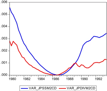
37 .000 .001 .002 .003 .004 .005 .006 1980 1982 1984 1986 1988 1990 1992 VAR_JPSSM2CD VAR_JPDIVM2CD

Fig. 4. Variance of Simple Sum and Divisia M2+CD for Japan

Figure 4 illustrates the variation pattern of the simple sum and its Divisia counterpart. The volatility pattern seen in simple sum M2+CD is similar to one seen in the previous country cases (high volatility until the late 1980s followed by a stability period and then again high volatility up to 1993). However, the variation in Divisia monetary aggregates of M2+CD lose some momentum in the late 1980s and from the beginning of the 1990s, the trend returns to its previous course.

38

4. Econometric Methodology and Empirical Results for

Developed Countries

This section includes the methods employed in this thesis and the empirical assessment of the monetary aggregates (both simple sum and Divisia) of the developed countries (United States, United Kingdom, Euro Area and Japan). After presenting the relevant econometric methods used in this thesis and focusing on several studies that have tested the empirical validity of the new monetary aggregates, I have evaluated the empirical results of the tests applied in this thesis for these four developed countries.

4.1. Econometric Methodology

Since macroeconomists generally deal with time series data in their empirical study, the problem of non-stationarity arises because some financial time series are not stationary in their levels and many time series are mostly represented by first differences. In order to avoid the spurious regression problems resulted from these non-stationary series, it would be convenient to observe the linear combinations of such non-stationary series so as to check whether these combinations somehow reveal stationarity. In this context, unit root tests are applied in order to check whether the variables of interest reveal non-stationarity and then cointegration test is employed after detecting the existence of non-stationarity of the each time series.

Since the power of the individual or univariate unit root tests is restricted due to the short data span of the macroeconomic time series, it would be appropriate to construct a panel of time series and cross section dimension