Determining default spreads and probabilities of default for a sample of Turkish firms using the merton model of credit risk

(1)

DETERMINING DEFAULT SPREADS AND PROBABILITIES OF

DEFAULT FOR A SAMPLE OF TURKISH FIRMS USING THE MERTON

MODEL OF CREDIT RISK

AHMET TEK

İ

N ÖZCAN

104626025

İ

STANBUL B

İ

LG

İ

ÜN

İ

VERS

İ

TES

İ

SOSYAL B

İ

L

İ

MLER ENST

İ

TÜSÜ

F

İ

NANSAL EKONOM

İ

YÜKSEK L

İ

SANS PROGRAMI

ADVISOR

S

İ

NA ERDAL, M.A.

(2)

DETERMINING DEFAULT SPREADS AND PROBABILITIES OF

DEFAULT FOR A SAMPLE OF TURKISH FIRMS USING THE MERTON

MODEL OF CREDIT RISK

AHMET TEK

İ

N ÖZCAN

104626025

Tez Danı

ş

manının Adı Soyadı (

İ

MZASI) : ...

S

İ

NA ERDAL, M.A.

Jüri Üyelerinin Adı Soyadı (

İ

MZASI) : ...

Assoc.Prof.Dr. EGE YAZGAN

Jüri Üyelerinin Adı Soyadı (

İ

MZASI) : ...

ORHAN ERDEM

Tezin Onaylandı

ğ

ı Tarih

: ……….

Toplam Sayfa Sayısı : 47

Anahtar Kelimeler (Türkçe)

Anahtar Kelimeler (

İ

ngilizce)

1) Merton Modeli

1) Merton Model

2) Kredi Riski

2) Credit Risk

3) Temerrüte Yakınlık

3) Distance to Default

4) Temerrüte Dü

ş

me

İ

htimali

4) Default Probability

(3)

ABSTRACT

This paper examines the relation between the debt-to-equity ratio of a firm and the risk premium that a firm should pay over the risk-free interest rate on its fixed rate debt obligations. Default risk is the uncertainty of a firm’s ability to meet its obligation against its debtholders. Prior to default, there is no way to discriminate between firms that will default and those that will not. Therefore, firms pay a risk premium over a risk-free interest rate related to their default probability. In this study, I estimate the likelihood of default and the resulting risk premiums for a sample of Turkish firms using the Merton model.

(4)

TABLE OF CONTENTS

ABSTRACT ……… ii

TABLE OF CONTENTS ……… iii

1. INTRODUCTION ……….. 1

2. MERTON MODEL ………. 6

2.1 Assumptions of Black and Scholes Option Pricing ……….. 7

2.2 Merton’s Extension to Black and Scholes Equation …….………. 9

2.3 How Merton Makes Pricing on Risky Discount Bonds ………... 12

2.4 Moody’s KMV’s Practical Approach to Merton Model ………... 14

2.5 A Case: A Closer Look at What the Numbers Mean ………... 19

3. THE MODELING PROCESS ……….. 21

3.1 Assumptions ……….. 21

3.2 Steps to Follow ……….. 22

3.2.1 Estimation of Equity Volatility ………. 22

3.2.2 Estimation of Debt Volatility ………... 23

3.2.3 Estimation of Asset Value and Volatility ….……….… 23

3.2.4 Calculation of Distance to Default ………….……….. 23

3.2.5 Calculation of Default Probability ………... 23

3.2.6 Defining Risk Premiums on A Risky Discount Bond ………... 24

4. DESCRIPTION OF DATA ……….……….. 24

5. THE RESULTS: DISTANCE TO DEFAULT AND RISK PREMIUMS ….………... 32

5.1 Turkcell Iletisim Hizmetleri A.S. ……….……… 32

5.2 Vestel Elektronik Sanayi veTicaret A.S. ……….…………... 33

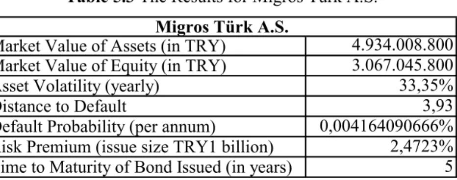
5.3 Migros Türk A.S. ………. 36

5.4 Anadolu Efes Biracılık ve Malt Sanayi A.S. ……….. 37

5.5 Ford Otomotiv Sanayi A.S. ……….……… 39

6. CONCLUSION ………..… 45

(5)

1. INTRODUCTION

The purpose of this study is to demonstrate the Merton model applied on Turkish firms. The Merton model is used as a credit risk assessment technique in many financial areas, and the credit rating agency Moody’s applies this model in its risk measurement tool. One crucial aspect of my study is that, whilst this model has been applied to many developed countries’ firms, it has not been used as a way of measuring credit risk in Turkey. The lack of data for publicly traded Turkish firms is the main reason of Merton model’s not being applicable. The other reason is corporate bond issuance has not been a widely used way of raising capital in Turkey. In recent years, the number of publicly traded Turkish firms has increased, and due to stable economic climate their balance sheets have become stronger. In light of all these developments, I did succeed in determining default probabilities of several large Turkish firms and to determine the risk premiums on their bonds.

The results that I obtain in this study can be used to price a public bond issue by these firms. They would not only help to define the risk premiums on a corporate bond, but also to assess credit risks and default probabilities of the firms..

Credit risk is defined as the potential that a counterparty will fail to meet its obligations in accordance with agreed terms. This case occurs when the counterparty defaults, where the debtor has not meet its obligation according to debt contract. The term default should be distinguished from the terms “insolvency” and “bankruptcy”. "Insolvency" is a legal term meaning that a debtor is unable to pay his debts. "Bankruptcy" is a legal finding that imposes court supervision over the financial affairs of those who are insolvent or in default.

What is default risk? Default risk is the uncertainty of a firm’s ability to meet its

obligations to its debtholders. Firms pay default premiums over a risk-free interest rate to compensate lenders for this risk. Basically, default probability of the firm determines the default premiums for all of the firm’s debt obligations. Mainly, default probability of a firm depends on three factors; 1. Market Value of Assets, 2. Business Risk (Asset Risk), and 3. Debt to Equity ratio (or the leverage). The default risk or the probability of a firm increases when the book value of its liabilities approaches to its market value of assets. And a firm defaults when the firm is unable to meet its obligations to its debtholders.

(6)

Amongst the alternative ways of credit risk measurement I choose the Merton model, since its result is observable continuously in time and it is easy to find cross-sectional data for publicly traded firms. On the other side, it is getting harder to use Merton model when firm balance sheets are more complicated with multiple types of debt with different maturities. The other widely used methods are Altman’s Z score, Credit Risk Plus and Credit Metrics. Altman’s Z score is developed in 1968 by Edward Altman, and attempts to quantify the health of a corporation through a linear combination of financial ratios.

WorkingCapitals/TotalAssets measures trend of losses, RetainedEarnings/TotalAssets measures historic profitability and reinvestment, EBIT/TotalAssets measures leverage and tax adjusted profitability, ValueOfEquity/TotalLiabilities measures solvency (market value of public companies, book value of private companies), and NetSales/TotalAssets measures profitability. Each ratio has a coefficient depending on whether the firm is public or

private.

A publicly traded firm is healthy if its Z score is above 2.99 and unhealthy if its Z score is below 1.81. Similarly, a private firm is healthy if its Z score is above 2.60 and unhealthy if its Z score is below 1.10. Z Scores vary by industry implying adjustments for industry even beyond the manufacturing / non-manufacturing distinction may be warranted.

Credit Risk Plus was proposed as a methodology by Credit Suisse in 1998 for calculating Value-at-Risk (VaR). It utilizes ideas that are well established in the insurance industry. This model shows that, if certain assumptions were made, the total loss probability distribution can be calculated analytically. Monte Carlo simulations are used. The

following steps are needed: sample an overall default rate, calculate a probability of default for each category, sample a number of default for each category, sample a loss for each default, calculate total loss, and repeat these steps many times. This procedure enables the estimation of the probability distribution of losses arising from defaults.

CreditMetrics was proposed by J.P. Morgan in 1997. The methodology is based on an analysis of credit migration, which tries to measure the probability of a company moving from one rating category to another during a certain period of time. A rating transition matrix is used for this process which indicates that the percentage probability of a bond moving from one rating category to another during a one-year period. In case of a bank with a portfolio of corporate bonds, calculating a one year VaR for the portfolio using

(7)

CreditMetrics involves carrying out Monte Carlo simulations of rating transitions for bonds in the portfolio over a one-year period. On each simulation trial the final credit rating of all bonds are calculated and the bonds are revalued to determine total credit losses for the year.

The methods other than Merton model are difficult to implement. Credit events are captured by changes in continuous default probabilities in Merton Model and risk drivers are asset values. Transition probabilities are driven by individual risk structures. However, approaches such as CreditMetrics and Credit Risk Plus are based on the credit migration approach which makes prediction difficult, unless one has the rating transition matrix for a sample of companies. With few historic data and default events in Turkey, it is not possible to develop such a matrix.

Therefore, my ultimate aim in this study is to prove that Merton model can be applied to Turkish firms, probability of default (PD) can be calculated, and risk premiums on TRY denominated corporate bonds can be easily calculated.

In order to demonstrate Merton model, I choose five publicly traded Turkish firms. These are: Turkcell İletişim Hizmetleri A.Ş. , Vestel Elektronik Sanayi ve Ticaret A.Ş. , Ford Otomotiv Sanayi A.Ş. , Anadolu Efes Biracılık ve Malt Sanayi A.Ş. and Migros Türk A.Ş. All five are listed on the Istanbul Stock Exchange and all financial data are available to the public.

The lack of long data sets for publicly traded Turkish firms is one of the challenging parts of this study. Therefore, in order to overcome this problem, I use the data set between 2001 and 2006.

The Istanbul Stock Exchange does publish balance sheet of each publicly traded firms at the end of each quarter. I work with the annual data, using year-end figures. As an accounting procedure, I make necessary adjustments on the data set, since before 2004 inflation indexing was applied to balance sheets in Turkey. This adjustment has made the reliability of my analysis stronger.

(8)

By using the number of outstanding shares at the end of each year and the year end share price (in TRY), I calculate market values of equity. Some of the firms that I work on had paid dividends during the time period of analysis. Therefore, I make necessary corrections on the price data set, and also take into consideration the dividend payments. The next step is to calculate total liabilities. I simply add up long term liabilities and short term liabilities for each year. However, the cash and cash equivalents item in the balance sheet is deducted from total liabilities amount where the item is a buffer for a firm in case of a default. So, I net off this effect. Also, for the reliability of my analysis, I deduct this amount from the market value of assets, too. I find the market value of each firm by adding up the total liabilities and the market value of equities. Debt to Equity ratios are derived at the end of these steps.

Given the price data of stocks with necessary dividend adjustments, I calculate the annual volatility of each stock by using the EWMA method. I also calculate the annual volatility of debt given yield changes of 1 year T-bills starting from year 2003 to 2006. Monthly volatility of debt is converted into yearly volatility. Underlying asset volatility implied by the market value and underlying asset value are derived by using the market value of equity, volatility of equity, the book value of liabilities, volatility of debt and the market value of asset.

In the final step, the Merton model is applied to each firm and conclusion is made. I try to estimate distance to default and probability of default numbers, and my conclusion is in line with the essence of Merton model. Amongst the five firms, default probabilities are higher with high debt to equity ratio firms and so higher risk premiums are assigned to them. And, with respect to this fact, long term borrowing is safer for high debt to equity firms since risk premium is getting tighter with time. All my findings will be broadly analyzed in the following sections.

The assessment of credit risk has always been important to banks and other financial institutions. Banks have been devoting significant resources for the last two decades to determine the potential amount of loss that would occur as a result of a credit default as accurately as possible. This trend is in part encouraged by the Basel Accords, Basel I and Basel II.

(9)

In 1988, the Basel Committee (BCBS) in Basel, Switzerland, published a set of minimum capital requirements for banks. This was a committee of G-8 central bankers. The aim was to build a strong and stable financial markets by ensuring that lenders were capitalized enough to protect their depositors. But, the first Basel Accord is now being replaced by Basel II. The reasoning behind the replacement is to keep pace with the increased

sophistication in financial markets and risk management. Also, under the rules of Basel I, lenders have been able reduce required capital where Basel II will align required minimum capital more closely with lenders’ risk profile.

Basel II allows banks to use their own risk management models to calculate required regulatory capital. Why do financial institutions need to hold regulatory capital? They do, because they take funds from savers and lend them on to borrowers. Since, there is always a probability of not getting some of the funds lent, they need capital of their own to protect their depositors.

Given the fact that Basel II aims to use modern risk management techniques, and takes a more sophisticated approach to credit risk, it allows banks to make use of internal ratings based approach – or “IRB Approach”, to calculate their capital requirements for credit risk. Parallel to international developments, after the implementation of Basel II requirements in Turkey, the strength and the competitiveness of the financial sector would be positively affected. Hence, banks and other financial institutions, being aware of the needs and capabilities of the sector, have started to devote more resources to implement and develop their internal risk management tools.

The system, a financial institution’s internal tool to assess credit risk, must involve at the very least a method of determining the probability that a counterparty will default (PD). One of these methods that are widely used in practice is the one based on the Merton model, an important theoretical model developed in 1974 by Merton and adapted by credit rating firms such as Moody’s for the practical assessment of credit risk.

The model adopted by Robert C. Merton is a structural credit risk model, where treats equity as an option on the firm's assets. It considers total liabilities as the strike price, total value of the firm’s assets as the value of the underlying asset and the equity as the call option. If at maturity, the firm’s asset value is greater than the promised debt payment,

(10)

debtholders get the promised amount and the equity holders get the residuals on asset value. But, in the worst case, when the asset value of the firm falls below the promised value to debtholders, firm defaults. Debtholders get all asset value, but equity holders get nothing.

In this study, my aim is to identify the essence of credit risk by analyzing how debt to equity ratio of a firm affects its default probability. By analyzing the annual financial reports of five Turkish firms, I attempt to determine risk premiums on the debts of these firms. I follow the methodology applied by Moody’s KMV, following the theoretical route drawn by Merton, and estimate distance to default measures and default probabilities for each of the firms. Equity volatilities and debt volatility are calculated by using EWMA method, and asset volatility is derived instantaneously with the given confidence level.

2. MERTON MODEL

In his precise study, Merton (1974) proposes a way of relating the capital structure of the firm with the credit risk. Although, his study is an extension to the one found by Black and Scholes (1973), the way they relate both credit risk and the capital structure is same. This model assumes that a company has a certain amount of zero-coupon debt that will become due at a future time T. The value of the firm’s assets is assumed to follow a lognormal distribution with constant volatility, and there are two classes of securities: debt and equity (where equity receives no dividend). In order to implement a Merton model, the current value of firm’s assets, the volatility of the company’s assets (instantaneously derived from an equation by using D/E ratio and the equity volatility), the outstanding debt and debt maturity is needed. The firm defaults if the value of its assets is less than the promised debt repayment at T.

The equity of the firm is a European call option on the assets of the company with maturity T and a strike price equal to the face value of the debt. If at maturity, T, the firm’s asset value is greater than the promised debt payment, debtholders get the promised amount and the equity holders get the residuals on asset value. But, in the worst case, when the asset value of the firm falls below the promised value to debtholders, firm defaults. Debtholders get all asset value, but equity holders get nothing. The model can be used to estimate either the risk-neutral probability that the firm will default or the credit spread on the debt.

(11)

As Merton stated, the value of corporate debt depends on three properties: i. The required rate of return on a riskless debt,

ii. The various provisions and restrictions included in the indenture,

iii. And, the probability of default, where the default probability defines the price changes between bonds.

Merton’s basic extension to Black and Sholes (1973) formula was that, he extended the option pricing formula of Black and Sholes and applied that in developing a pricing theory of corporate liability. Merton used this general equilibrium theory of option pricing since the final formula is a function of observable variables.

2.1 Assumptions of Black and Scholes Option Pricing

Before getting into details of Merton model, I would be explaining the main assumptions of Black and Scholes option pricing, and further to that would be exploring the extensions of Merton’s approach.

Assumptions of Black and Scholes option pricing; i. There are no transaction costs or taxes.

ii. There are sufficient numbers of investors with a certain wealth levels, and each can buy or sell as much of an asset as he wants to at the market price.

iii. Each investor can borrow or lend at the same rate of interest. iv. Short sale of an asset is allowed.

v. Trading in assets take place continuously in time.

vi. The Modigliani Miller theorem obtains (the value of a firm is invariant of its capital structure).

vii. There is no uncertainty regarding the term structure of interest rate, and it is flat. viii. The value of a firm can be described by a diffusion type stochastic process with stochastic differential equation

(12)

Where, _{α is the expected rate of return on the firm per unit of time,}Cis the total dollar

payouts by the firm per unit time to either its shareholders or liability holders, _σ2_{is the} variance of return, and dZis the Gauss-Wiener process.

From the assumptions listed above, assumptions i. and iv. stand for the “perfect market” case, and according to Merton, these assumptions can be weakened.

However, great importance is given to the assumptions vi. and vii. Assumption vi. indicates the Modigliani - Miller (1958) theorem, where it forms the basis for modern thinking on capital structure. The basic theorem states that, in the absence of taxes, bankruptcy costs, and asymmetric information, and in an efficient market, the value of a firm is unaffected by how that firm is financed. It does not matter if the firm's capital is raised by issuing stock or selling debt.

Modigliani – Miller theorem was originally proved under the assumption of no taxes (but, can be extended to the situations with taxes). There are two propositions of this model: the value of an unlevered firm is equal to the levered firm, and, the cost of equity is a linear function of firm’s debt to equity ratio. The first proposition holds, because instead of investing in a levered firm’s shares, an investor can invest in an unlevered firm and can borrow the same amount of money that the levered firm does from the market. The eventual return should be same to either of these investments. Second proposition holds, assuming expected return on equity as follows,

₀ (c₀ b) E

D c

y= + − (2.2)

Where, y is the cost of equity, c is the cost of capital for an all equity firm, ₀ b is the cost

of debt, and E

D is the debt to equity ratio of the firm. A higher debt to equity ratio requires higher rate of return on equity because of the higher risk involved for equity-holders in a company with debt.

Assumption vii. is relevant with “Efficient Market Hypothesis” of Fama (1970). The efficient market hypothesis states that it is not possible to consistently outperform the

(13)

market by using any information that the market already knows, except through luck. Efficient market hypothesis claims that investors have rational expectations that on average the population is correct. And, when a new information appears in the market related with the investment strategy, people revise their expectations. Black and Scholes assumes that, the yield curve is flat and known with certainty. This means, given the riskless rate of return , r , same for all time, present value of a riskless discount bond can be calculated. Assumption viii. indicates that the value of firm follows a stochastic process, and the price movements are continuous where returns on securities are independent. This assumption is in line with the “Efficient Market Hypothesis”.

Given the assumptions, I can start to explore how Merton extended Black and Scholes equation, and calculated risk premiums on risky discount bonds.

2.2 Merton’s Extension to Black and Scholes Equation

Merton assumes that, there exists a security, and it is simply a function of the value a firm and time, Y =F( tV, ). And, the dynamic of this security’s value can be written in

stochastic differential equation form.

dY =

[

αyY −Cy

]

dT +σyYdzy (2.3)

In this stochastic differential equation, αy is the instantaneous expected rate of return per

unit time on the security, C is the dollar payout per unit time to this security, y 2 y

σ is the instantaneous variance of return per unit time, and dz is the Standard Gauss – Wiener y

process.

As Merton states, there stands an explicit functional relationship between dV and dY .

Given )Y =F( tV, , using Ito’s Lemma, we can rewrite the equation for Y as,

dY =FvdV + Fvv

( )

dV +Ft 2 2

1

(14)

dY σ V F_vv

(

αV C

)

F_v F_t dt+σVF_vdz ⎥⎦ ⎤ ⎢⎣ ⎡ ₊ ₋ ₊ = 2 2 2 1 (2.4b)

where subscripts denote partial derivatives.

_yY = _yF ≡ V F_vv +( V −C)F_v +F_t +C_y 2 1_σ2 2 _α α α (2.5a) σyY =σyF ≡σVFv (2.5b) dz_y ≡dz (2.5c)

In equation (2.5a), instantaneous returns on Y and V are perfectly correlated.

Then, Merton formulates a portfolio of three securities including a riskless debt, a particular security and the firm. Total investment in the portfolio is zero and that is achieved by using the proceeds of short sales and borrowing to finance long positions. If we denote W₁as the number of dollars invested in the firm, W₂ as the number of dollars

invested in the security, and W as the number of dollars invested in the riskless debt, there ₃ stands a relation between these securities

(

W₃ ≡−

[

W₁ +W₂

]

)

.

Let dxbe the dollar return of the portfolio,

(

)

_Y W rdt dt C dY W V Cdt dV W dx= ₁ + + ₂ ( + y )+ ₃ (2.6a) dx=

[

W1(α −r)+W2(αy −r)

]

dt+W1σdz+W2σydzy (2.6b) dx=

[

W1(α −r)+W2(αy −r)

] [

dt+ W1σ +W2σy

]

dz (2.6c)

(15)

Merton assumes that for W_j =W_j_*, dzis always zero, then dx* becomes nonstochastic.

Since, the portfolio requires zero net investments, the equation also should avoid the arbitrage profits. As a result,

W₁σ +W₂σy =0 (no risk case) (2.7a)

W₁

(

α −r)+W₂(αy −r

)

=0 (no arbitrage case) (2.7b) Given the equations for no risk and no arbitrage cases, Merton says that a nontrivial

solution exists if and only if,

_⎟⎟ ⎠ ⎞ ⎜ ⎜ ⎝ ⎛ − = ⎟ ⎠ ⎞ ⎜ ⎝ ⎛ − y y r r σ α σ α _(2.8)

By using equation (2.5a), Merton substitutes equation (2.8) as follows,

v y t v vv VF rF C F F C V F V r σ α σ σ α ⎟⎠ ⎞ ⎜ ⎝ ⎛ ₊ ₋ ₊ ₊ ₋ = − 2 ( ) 1 2 2 (2.9a) = V Fvv +(rV −C)Fv −rF+Ft +Cy 2 1 0 _σ2 2 _(2.9b)

Merton states that, this final equation (2.9b) must be satisfied by any security which is a function of value of the firm and time. There should of course be boundary conditions to distinguish one security from another, and he specifies two boundary conditions and an initial condition.

As clearly can be seen in equation (2.9b), value of a security depends on many variables. Value of a firm is a function of time, interest rate, the volatility of firm’s value, the payout policy of the firm, and the promised payout policy to the holders of the security. Whereas, it is not a function of expected rate of return of a firm, risk preferences of investors or the characteristics of other assets available. This conclusion is important, in case it shows us

(16)

that two investors with different utility functions and different expectations about the future value of a firm, but who can agree on the volatility of the firm value with given interest rate and current firm value, would agree on the value of a particular security, F .

2.3 How Merton Makes Pricing on Risky Discount Bonds

Merton applies the formula to a simplest case, and assumes that the firm has two classes of claims: debt and the residual claim, equity. Then, he sets some certain provisions and restrictions on the indenture of the bond issue. First, the firm promises to pay a total of

B dollars to the bondholders on the specified calendar date, T . Second, if at T the payment is not made, bondholders take over the company. Third, the firm cannot issue any new senior (or equivalent rank) claims on the firm, nor can it pay the cash dividends or do share purchase prior to the maturity of the debt.

If F is the value of the debt issue, the following equation could be written,

0 2 1 2 2 ₊ ₋ ₋ ₌ t v vv rVF rF F F V σ (2.10) Since there is no coupon payment Cy =0. C =0, given the equation (2.5a). And, time to maturity isτ =T−t, so thatF_t =F_τ. In order to solve for equation (2.10), two boundary and an initial condition must be met. These are derived from the provisions of the

indentures and the limited liability of claims. V ≡F(V,_τ)+ f(V,_τ)V, where f is the value of the equity. The following equations show the boundary conditions;

F(0,_τ)₌ f(0,_τ)₌0 (2.11a)

F(V,τ)/V _≤1 (2.11b)

The second above shown equation implies the regularity condition, and substitutes fort he other boundary condition in a semi-infinite boundary problem where0≤ V ≤∞. As Merton discussed, initial condition is derived from indentures .i and .ii and the fact that

(17)

maturity dateT ,V

( )

T 〉B bondholders should be paid, where the value of the equity would

be V

( )

T − B〉0. If the bondholders are not paid, then, that means value of equity is zero. WhenV

( )

T ≤B, the firm defaults, equity holders would pay additional money. As a result,

initial condition for the debt at τ =0 isF(V,0)=min

[ ]

V,B .

If the value of the equity is f(V,_τ)=V −F(V,_τ), and equations (2.10) and (2.11b) are used to substitute for F , then the partial differential equation becomes as follows,

0 2 1_σ2 2 ₊ ₋ ₋ _τ ₌ f rf rVf f V vv v (2.12)

and, this equation is subject to boundary conditions, plus f(V,0)=max(0,V −B).

Merton used all these equations to show that pricing of an equity is the pricing of an European call option on non-dividend paying common stock. And, states that, a firm’s current price as the spot price and the value of the bond as the strike price. With a constant volatility, _σ2_{, Black-Scholes equation should hold,}

f(V, ) V (x1) Be (x2) r φ φ τ ₌ ₋ −τ (2.13a)

∫

∞ − ⎥⎦ ⎤ ⎢⎣ ⎡− ≡ x dz z x 2 2 1 exp 2 1 ) ( π φ (2.13b) _σ _τ _σ _τ ⎭ ⎬ ⎫ ⎩ ⎨ ⎧ + + ⎥⎦ ⎤ ⎢⎣ ⎡ ≡ ) 2 1 ( log 2 1 r B V x (2.13c) x2 ≡x1−_σ _τ (2.13d)

Given equation (2.13a) andF =V − f , value of the debt issue can be written as,

[ ]

[

(

)

]

[

(

)

]

⎭ ⎬ ⎫ ⎩ ⎨ ⎧ ₊ = − _φ _σ _τ _φ _σ _τ τ τ 2 1 2 2 , 1 , , h d d d h Be V F r (2.14)

(18)

where, V Be d ≡ −rτ (2.15a) τ σ τ σ τ σ ⎥⎦ ⎤ ⎢⎣ ⎡ ₋ − ≡ ) log( 2 1 ) , ( 2 2 1 d d h (2.15b) τ σ τ σ τ σ ⎥⎦ ⎤ ⎢⎣ ⎡ + − ≡ ) log( 2 1 ) , ( 2 2 2 d d h (2.15c)

Merton, then rewrites the equation (2.14) in the following form because it is common to talk about yield rather than prices in bond discussions,

[

]

[

]

⎭ ⎬ ⎫ ⎩ ⎨ ⎧ ₊ − = − φ σ τ φ σ τ τ τ 2 1 2 2 ( , 1 , ( log 1 ) ( h d d d h r R (2.16)

where, R(_τ) is the yield to maturity on the risky debt, and R(τ)−rstands for the risk premium on a risky discount bond. Risk premium is crucial in case it shows the risk structure of interest rates. As shown in the equation (2.16), risk premium depends on two factors: the volatility of the firm’s operations and

V Be

d = −rτ .

Merton’s comparative statics analysis of the risk structure proves that the value of debt is an increasing function of current market value of the firm and the promised payment at the maturity. Whereas, it a decreasing function of time to maturity, the business risk of the firm (or the volatility), and the riskless rate of return.

2.4 Moody’s KMV’s Practical Approach to Merton Model

One of the world’s leading providers of the credit analysis Moody’s KMV uses a

comprehensive version of Merton model for credit risk assessments. In addition to default probability of a debt, there is also a probability of default on other asset classes that a firm

(19)

invested in. In that manner, Moody’s KMV uses an effective way of portfolio

management, since default correlations are measured. That makes a difference between standalone risk and portfolio risk. The default risk or probability of a firm increases when the book value of its liabilities approaches to its market value of assets. And a firm defaults when the firm is unable to meet its obligations against the debtholders. However, as

indicated in KMV’s studies of default cases, default point generally lies between the total liabilities and short-term liabilities, since long term liabilities provide a firm with some buffer. Therefore, the net worth of a firm is the difference between the Market Value of Assets and the default point. A firm defaults when the market net worth reaches to zero. This fact is closely related with business risk (where asset volatility depends on the size and the nature of firm’s business risk). One important conclusion that KMV made shows that asset volatility tends to be lower for high leveraged firms.

KMV uses a way to combine three components of the default probability into a single measure, which compares the market net worth with the asset volatility.

[

] [

]

[

MarketValueOfAssets

] [

AssetVolatility

]

DefaultPo eOfAssets MarketValu t ceToDefaul Dis * int tan = − (2.17)

Given the way of setting distance to default, the next step is to collect all relevant

information about the firm as possible. All financial statements of a publicly traded firm, market price of its debt and equity and subjective appraisals of the firm’s prospects and risks are basic types of information available.

Moody’s KMV used Vasicek-Kealhofer Model (1989) to combine all these factors and to find distance to default and default probability of a firm. This model is an extension to Black-Scholes-Merton model, and assumes a firm’s equity as a perpetual option with the default point acting as the absorbing barrier for the firm’s asset value. When the asset value hits the default point, the firm is assumed to default. Also, the model allows more specified liabilities instead of two kind used in Merton model.

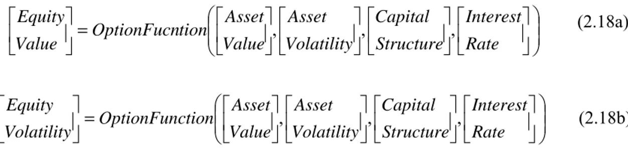
Given the equity volatility, asset volatility can be estimated as Merton model and Vasicek Kealhofer model both state that equity is a call option on the firm’s assets with a strike price equal to the book value of firm’s liabilities (equity holders have the right, but not the

(20)

obligation, to payoff debtholders and take over the remaining assets of the firm). This process is similar to defining implied volatility of an option given the option price. The more volatile is the asset price, the greater is the chance of high asset values. And that indeed means higher payouts for equities. KMV formulates this equations as follows;

(2.18a) _⎟⎟ ⎠ ⎞ ⎜⎜ ⎝ ⎛ ⎥ ⎦ ⎤ ⎢ ⎣ ⎡ ⎥ ⎦ ⎤ ⎢ ⎣ ⎡ ⎥ ⎦ ⎤ ⎢ ⎣ ⎡ ⎥ ⎦ ⎤ ⎢ ⎣ ⎡ = ⎥ ⎦ ⎤ ⎢ ⎣ ⎡ Rate Interest Structure Capital Volatility Asset Value Asset tion OptionFunc Volatility Equity , , , (2.18b)

All in hand, we can list some variables that determine the default probability of a firm over a time period, from now until time T:

i. The current asset value (V ), ₀

ii. The distribution of the asset value at time T, iii. The volatility of future asset value at time T, iv. The book value of liabilities,

v. The expected rate of growth in the asset value over the time period, vi. The length of the period, T.

Figure 2.1 Estimation of Expected Default Frequency

In that respect, the relation between default point and the probability of default becomes crucial. For the distribution of asset values, neither normal nor lognormal distributions can be used (the normal distribution is not an accurate measure to define the probability of

⎟⎟ ⎠ ⎞ ⎜⎜ ⎝ ⎛ ⎥ ⎦ ⎤ ⎢ ⎣ ⎡ ⎥ ⎦ ⎤ ⎢ ⎣ ⎡ ⎥ ⎦ ⎤ ⎢ ⎣ ⎡ ⎥ ⎦ ⎤ ⎢ ⎣ ⎡ = ⎥ ⎦ ⎤ ⎢ ⎣ ⎡ Rate Interest Structure Capital Volatility Asset Value Asset tion OptionFucn Value Equity , , ,

(21)

default, since default point is in reality a random variable and firm adjusts their liabilities as they near default). Difficulties arising from any adverse changes in asset values or the leverage ratio of the firm, and the relations with the default point would definitely deteriorate the determination of default probability. And, changes in asset value and the leverage ratio can be highly correlated. Therefore, Moody’s KMV first measures the distance to default, the number of standard deviations the asset value is away from default, and than uses the empirical data to determine the corresponding default probability

(Moody’s KMV determines the relationship between the distance to default and default probabilities by looking at the historical default and bankruptcy frequencies). For my study, since I do not have any empirical data set of default and bankruptcy frequencies, I will be relying on the variables available to us.

As stated, Moody’s KMV uses Vasicek-Kealhofer model to calculate Expected Default Frequency (EDF) credit measure rather than using Merton’s option pricing method. One important expression is mentioned here to derive the asset volatility given equity volatility.

A E A E V V d N σ σ ₌ ( 1) _(2.19)

where, σ is the equity volatility, E VA is the value of the firm, VE is the value of the equity

and σ is the firm’s volatility. However, as stated by Moody’s KMV, the model linking A

equity and asset volatility holds only instantaneously. In practice, the market leverage moves around for too much for to provide reasonable results. For example, if the market leverage is decreasing quickly then will tend to overestimate the asset volatility and thus the default probability will be overstated as the firm’s credit risk improves.

Therefore, in this study, given the equity and the debt volatilities I calculate the asset volatility of a firm accordingly;-

D A D E A E A V V V V σ σ σ = + (2.20)

(22)

The probability of default is the probability that the market value of the firm’s assets will be less than the book values of the firm’s liabilities by the time debt matures. Black Scholes model assumes that the random component of the firm’s asset is normally distributed, )ε ≈ N(0,1 . Then, distance to default and the default probability can be calculated as, t t X V DD A _A t A μ σ ) /σ 2 ( ln 2 ⎥⎦ ⎤ ⎢⎣ ⎡ ₊ ₋ = (2.21a) t t X V N p A _A t A t (μ σ 2) /σ ln 2 ⎥⎦ ⎤ ⎢⎣ ⎡ ₊ ₋ − = (2.21b)

where _μ is the expected return on firm’s assets, V_A is the asset value, σ2_A is the volatility

of the asset, and X is the value of total liabilities. _t

As known and stressed by Moody’s KMV, the normal distribution is poor choice to define the probability of default since the default point is in reality a random variable and firm adjusts their liabilities as they near default. But for my study, I am unable to define the nature of liabilities.

One other important aspect of Merton model is that, it assumes the equity market is efficient. Efficiency means market price reveals all relevant information about the firm’s value. However, in reality, it is difficult to capture a pure information set prices in the asset value in the market.

To sum up, the Vasicek-Kealhofer model has the same conceptual architecture as the Merton approach, but brings practicability for banks and lenders who wished to assess default probability. Unlike Merton model, KMV allows liabilities to include current liabilities, short term debt, long term debt, convertible debt, preferred stock, convertible preferred stock, and common equity. In the Merton model, default occurs when the firm value is lower than the debt to be paid at the maturity. However, in the Vasicek – Kealhofer model default can happen even before the maturity of a particular debt issue. And, equity is modeled as a perpetual option. The firm value is only modeled as a

(23)

geometric Brownian motion for the purpose of calculation of the unknown input variables and the distance to default. As a result, the practicability of KMV model enables risk managers to monitor public companies on a daily basis and use the estimated default probability as early warning information.

Following the route defined above, throughout my study, I will be analyzing some Turkish conglomerates from non-financial sector, and would try to foresee default cases without mitigation risks. Given the fact that Turkish financial sector is not healthy and liquid enough for corporate debt issuance, I will try to estimate risk premiums on standalone basis.

2.5 A Case: A Closer Look at What the Numbers Mean

In this section, I will be explaining what all those numbers mean in a very simple case. Let’s assume Firm A which has only one class of debt and one class of equity, and will be wound up after two years.

Table 2.1 Assets and liabilities of Firm A Assets Liabilities

By the nature of limited liability feature of equity, equity holders have the right, but not the obligation, to pay off the debt holders and take over the remaining assets of the firm. Thus, equity is a call option on the firm’s assets with a strike price equal to the book value of the firm’s liabilities. Therefore, by using the option nature of the equity, underlying asset volatility implied by the market value and underlying asset value can be derived by using the market value, volatility of equity, and the book value of liabilities. This process is

50

40

(24)

similar to the one used by option traders in market cases, where the implied volatility is derived from the observed option price.

Now, in my case, let’s assume Firm A borrows $40 from a bank and $10 is invested by the owners. And, $50 is invested in equities. What is value of the equity after two years? The answer is completely related with the value of the assets. If the value of assets is $30 after two years, then the value of equity will be zero. Whereas, if the value of assets is $60, then the value of equity is $20. Obviously, Firm A can choose to mark to market its equities after a year, and let’s assume it is $40. Whilst, it is $40, I cannot say the value of the equity is zero just because the value of assets can increase above $40 in a year’s time (when the Firm A is wound up). This fact proves that the higher the volatility of assets the greater is the chance of high asset values. The more volatile assets have higher probabilities of high values, and thus create high payouts for the equity. Conversely, high volatile assets can create lower asset values, because volatility works in either case. However, this does not affect the equity value, since equity holders receive nothing after two years if the value of assets is less than $40. So, where does the increase in the equity’s value come from? It comes from bank holding Firm A’s debt. The only way the value of equity can increase while the asset value remains constant is to take the value from the market value of debt. When the Firm A’s assets are reinvested in higher-risk equities, this would increase the default risk of debt and reduce its market value.

As indicated in the example, the value of debt and the value of the equity is closely related. Due to option nature of the equity, Merton model helps us solve the problem by observing the value of the equity, and solve backwards the market value of assets. The two unknown parameters asset value and asset volatility can be solved with values implied by the equity value, equity volatility and the capital structure (in practice, there are more complex capital structures and situations).

After all, let’s assume that Firm A is 1.5 standard deviation away from default. That is, it would take 1.5 standard deviation move in the asset value of Firm A before it would default. The distance to default measure combines key credit issues: the value of firm’s assets, its business risk and the leverage. Whereas, default probability can be easily computed from distance to default if the probability distribution of asset is known.

(25)

3. THE MODELING PROCESS

To determine whether a company has the ability to generate sufficient cash to service its debt obligations the focus of the credit analysis has been on the company’s fundamental accounting information. Industrial environment, investment plans, balance sheet data and management skills help with the evaluation of the companies’ likelihood of survival over a time horizon or over the life of the outstanding liabilities. A firm’s financial statement analysis enables to see a true financial condition and future prospects. Since, accounting principles are backward oriented, accounting information does not include a precise concept of future uncertainty. As a result, a market valuation of firm’s assets is difficult in the absence of actual market related information.

In this study, by using the Merton model and extending its formula with the KMV’s approach, I priced publicly traded five Turkish firms’ debt assuming that all Merton’s arguments holds and the results can serve to find out related default probabilities.

Balance sheet data is used to get required data set for my analysis. Balance sheets, from the data store of Istanbul Stock Exchange starting from year 2001 to 2006, of Turkcell İletişim Hizmetleri A.Ş., Vestel Elektronik Sanayi Ve Ticaret A.Ş., Ford Otomotiv Sanayi A.Ş., Anadolu Efes Biracılık Ve Malt Sanayi A.Ş. and Migros Türk A.Ş. are scrutinized, and by using the necessary data set market value of each firm is calculated. In order to get an accurate result, I deducted cash and cash equivalents from the market value of assets and total liabilities where the item is a buffer for a firm in case of a default. All price data is get from Bloomberg (data provider) and repriced regarding the dividend payments per share. Risk free interest rate is 20,58% (interest rate of T-bill maturing on December 12, 2007 at the end of 2006).

3.1 Assumptions

As a main concept and defined by Merton, I assumed that all of the company’s liabilities are zero – bonds with the same maturity. Besides that, as listed under section II, basic assumptions should hold. These are; the market is perfect, the risk free rate is constant, the company has only two classes of claims: a single homogeneous class of debt (zero bonds all with same seniority and maturity), and the residual claim, equity. The firm is not

(26)

allowed to issue a new debt not pay cash dividends nor repurchase shares prior to the maturity of the debt, the Modigliani – Miller theorem obtains, and the value of the firm follows a diffusion type stochastic process (where the volatility of the returns on firm value is constant over time and the distribution of its growth rates is normal).

3.2 Steps to Follow

By using Merton model, I define the risk premium on a risky discount bond. But, before the calculation, there are some steps in the determination of the default probability of a firm;

3.2.1Estimation of Equity Volatility: As it is known, the financial asset returns have a non – normal distribution, and it is leptokurtic, with the tails fatter than those of the normal distribution. Given that fact, for the estimation of the equity volatility of a publicly traded firm, I used Exponential Weighted Average Method (EWMA).

2 1 2 1 2 ₍₁ ₎ − − + − = t t t λσ λ r σ (3.1) In the equation, 2 1 − t

σ is a dispersion estimate for day t, 2 t

σ is a dispersion estimate for day 1

−

t calculated at the end of day t, λ is the decay factor, and r is the asset’s return for _t2₋₁ the day t−1 and the return for day t is calculated as natural logarithm of the ratio of a stock price from the day t to previous day t−1.

The EWMA model allows one to calculate a value for a given time on the basis of the previous day’s value. The EWMA model has an advantage, because it has a memory. The EWMA remembers a fraction of its past by the decay factor, _{λ , that makes it a good} indicator of the history of the price movement if a wise choice of the term is made. Using the exponential moving average of historical observations allows to capture the dynamic feature of volatility. The model uses the latest observations with the highest weights in the volatility estimate.The exponential weighted moving average method depends on the decay factor,_λ

(

0<λ<1

)

. This parameter defines a relative weight (1_{− that is applied to the}_λ) latest return. This weight also defines the effective amount of data used in estimating volatility. The more the _{λ value, the less last observation affects the current dispersion}

(27)

estimation. Also, the greater the value, the faster dispersion will come back to previous level after strong return change. The optimal value for current daily volatility isλ =0.94. By using the Bloomberg, I obtained stock price data of each firm and made corrections on these data regarding dividend payments. Then, the next step was to estimate volatility with EWMA method. The result is checked with Chi-Square test.

3.2.2 Estimation of Debt Volatility: I calculate the annual volatility of debt given yield changes of 1 year generic T-bills starting from year 2003 to 2006. Monthly volatility of debt calculated with EWMA method is converted into yearly volatility.

3.2.3 Estimation of Asset Value and Volatility: The asset value and asset volatility of the firm is estimated from the market value and volatility of equity, the book value of

liabilities, and the volatility of debt.

3.2.4 Calculation of Distance to Default: The distance to default is calculated from the asset value and asset volatility, and the book values of liabilities. As discussed in section II, asset value, future asset distribution, asset volatility and the level of the default point are the critical variables of default case. If the value of the firm falls below the default point, then the firm defaults. Therefore, the probability of default is the probability that the asset value will fall below the default point. The final result of my distance to default analysis is the measure of the number of standard deviations the asset is away from default.

3.2.5 Calculation of Default Probability: Although it is certain that historical data and bankruptcy frequencies are needed in order to obtain relationship between distance to default and default probability, the main assumption of my study requires that distance to default is normally distributed. Normal distribution of distance to default gives us the default probabilities.

Whilst there are differences in default rates across industry, time, and size, KMV has found that the relationship between distance to default and default frequency is constant across all these variables and it is captured by the distance to default measure.

(28)

3.2.6 Defining Risk Premiums on a Risky Discount Bond: For a given maturity, I

determine the risk premium on a risky discount bond, which shows the default probability of a firm embedded in the bond pricing. I show how the risk premiums change depending on the volatility of firm’s operations and the ratio of the present value (at the riskless rate) of the promised payment to the current value of the firm.

4. DESCRIPTION OF DATA

Determination of distance to default, default probabilities and risk premiums require detailed analyses of balance sheets and stock market information. Therefore, all information available should be scrutinized to foresee difficulties in estimations. In the tables below, I summarize all data used in pricing for the firms that are in my sample. Total liabilities are simply the sum of short-term and long-term liabilities for each year. Market value of equity is calculated by multiplying year-end share price with number of outstanding shares. All stock price information is obtained from data provider

Bloomberg, and dividend payments are taken into consideration for necessary adjustments. Dividend data are available in data storage of Istanbul Stock Exchange. I add up total liabilities and market value of equity to find market value of each firm. For the accuracy of my calculations of distance to default and default probabilities, I deduct cash and cash equivalents from total liabilities and market value of firms. Before 2004, inflation

indexation was applied to balance sheet data. Therefore, I use inflation indices to modify the necessary balance sheet information. The one-year risk free interest rate is 20,58%, which is the rate on a bond maturing in a year as of end of 2006. I use this rate since it is the risk free rate that could be used for my calculations.

Equity volatility is estimated by using the exponentially weighted moving average EWMA method. Monthly returns, modified with dividend payments, are used for monthly volatility estimations. Then these are converted into yearly figures by using the square root method. In order to prove the accuracy of my estimations, I run a chi-square test on the standard deviation of same data set regarding the degrees of freedom. I calculate the annual volatility of debt given yield changes of 1 year generic T-bills starting from year 2003 to 2006. Monthly volatility of debt is converted into yearly volatility. Yields of 1 year generic T-bills are obtained from data provider Bloomberg. The last data required for my

(29)

calculations was asset volatility. Underlying asset volatility implied by the market value and underlying asset value are derived by using the market value of equity, volatility of equity, the book value of liabilities, volatility of debt and the market value of asset.

D A D E A E A V V V V σ σ σ = + (4.1)

where, _{σ is the equity volatility,}_E V_A is the value of the firm, V_E is the value of the equity,

A

σ is the firm’s volatility, VD is the value of the debt and σ is the volatility of debt. D

Table 4.1 summarizes the data for Turkcell Iletisim Hizmetleri A.S. Total liabilities of this firm decreases starting from year 2001 to year 2006, and it is TRY 2,746,742,000 in year-end 2006. Whereas, market value of equity of this firm gradually goes up in between these years, and it is TRY 15,730,000,000 in year-end 2006. Along with the increase in market value of equity, market value of Turkcell reaches to TRY 18,476,742,000 compared to market value of TRY 12,840,646,272 in 2001. These outcomes indicates a significant decrease in debt to equity ratio of this firm from 1,0545 in year 2001 to 0.1746 in year 2006. The company becomes cash rich between these years, which create a cushion in case of bad financial conditions. Turkcell’s monthly equity volatility is 0.114365017 in year end 2006. Monthly debt volatility is fixed for all firms and it is 0.077582856. Due to low debt to equity ratio, monthly asset volatility is so close to equity volatility of this firm and it is 0.10889702. The yearly asset volatility is at 0.377230278 in year-end 2006.

Table 4.2 summarizes the data for Vestel Elektronik Sanayi ve Ticaret A.S. Unlike Turkcell, total liabilities of Vestel increase almost three times starting from year 2001 to year 2006. Total liabilities of Vestel is TRY 3,445,173,000 in year-end 2006 where it is TRY 1,165,923,303 in year-end 2001. Market Value of equity of this firm makes high in 2003, however, since then starts to decrease. There is almost no change in market value of equity in year-end 2006 compared to year-end 2001, where it is at TRY 585,487,584. Market Value of Vestel reaches to TRY 4,030,660,584 in 2006. As a result, debt to equity ratio of Vestel more than doubles from year 2001 to 2006, and it is 5,8843 in year-end 2006. Due to high debt holding, asset volatility of Vestel is lower, where monthly equity volatility is at 0.093022256, debt volatility is at 0.077582856 and monthly asset volatility

(30)

is at 0..79825559 in end 2006. The yearly asset volatility is at 0.276523849 in year-end 2006.

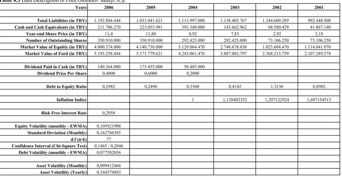
Table 4.3 summarizes the data for Ford Otomotiv Sanayi A.S. Ford has relatively stable total liabilities throughout the years I analyze. The average of total liabilities is TRY 1,135,564,438 between years 2001 and 2006, where it is TRY 1,192,884,444 in year end 2006. Whilst the total liability is stable, market value of equity of this firm goes up to TRY 4,000,374,000 in year-end 2006 from TRY 1,114,841,070 in year-end 2001. Therefore, the increase in market value of Ford can be attributed to change in market value of equity and it is TRY 5,193,258,444 in year-end 2006. Debt to equity ratio of this firm is at 0.2982 in year-end 2006 compared to 0.8902 in year-end 2001. Monthly equity volatility of Ford is at 0.105921908, debt volatility is at 0.077582856 and monthly asset volatility is at 0.099412466 in year-end 2006, where yearly asset volatility is at 0.344374883. Table 4.4 summarizes the data for Anadolu Efes Biracılık ve Malt Sanayi A.S. Total liabilities and market value of equity of Efes increase throughout the years with relatively stable debt to equity ratio. Total liabilities of Efes is TRY 386,716,680 in year-end 2001, and it is TRY 1,946,411,000 in year-end 2006. Market value of equity rises from TRY 1,806,029,088 in year-end 2001 to TRY 4,938,360,788 in year-end 2006. Therefore, market value of Efes rises more than three times, and it is TRY 6,884,771,788 in year-end 2006. Debt to equity ratio of Ford is 0.3941 in year-end 2006. Monthly equity volatility of Efes is at 0.089558051, debt volatility is at 0.077582856, and monthly asset volatility is at 0.086172513 in year-end 2006, where yearly asset volatility is at 0.298510342.

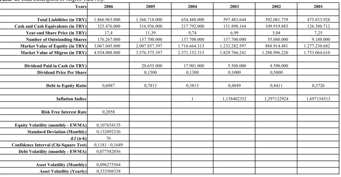
Table 4.5 summarizes the data for Migros Türk A.S. Total liabilities and market value of equity of Migros increase throughout the years. Total liabilities of Migros is TRY

475,833,928 in year-end 2001, and it is TRY 1,866,963,000 in year-end 2006. Market value of equity rises from TRY 1,277,230,682 in year-end 2001 to TRY 3,067,045,800 in year-end 2006. Therefore, market value of Migros gradually goes up and it is TRY 4,934,008,800 in year-end 2006. Debt to equity ratio of Migros increases from year 2001 to 2006 and it is 0.6087. Monthly equity volatility of Migros is at 0.107654135, debt volatility is at 0.077582856 and monthly asset volatility is at 0.096275564 in year-end 2006, where yearly asset volatility is at 0.333508338.

(31)

Years 2006 2005 2004 2003 2002 2001

Total Liabilities (in TRY) 2.746.742.000 2.002.709.000 3.192.851.000 3.677.812.725 4.883.287.247 6.590.644.272

Cash and Cash Equivalents (in TRY) 2.247.049.000 1.084.379.000 1.026.613.000 926.873.881 854.664.787 626.887.174,47

Year-end Share Price (in TRY) 7,15 6,91 6,30 3,18 2,20 2,84

Number of Outstanding Shares 2.200.000.000 1.854.887.341 1.474.639.361 500.000.000 500.000.000 470.348.717

Market Value of Equitiy (in TRY) 15.730.000.000 15.210.074.000 13.861.606.000 7.000.004.000 4.850.010.000 6.250.002.000,00

Market Value of Turkcell (in TRY) 18.476.742.000 17.212.783.000 17.054.457.000 10.677.816.725 9.733.297.247 12.840.646.272

Dividend Paid in Cash (in TRY) 509.075.111 250.127.565 118.158.605

Dividend Price Per Share 0,2745 0,1696 0,2363

Debt to Equity Ratio 0,1746 0,1317 0,2303 0,5254 1,0069 1,0545

Inflation Indice 1 1,138402352 1,297122924 1,697154513

Risk Free Interest Rate 0,2058

Equity Volatility (monthly - EWMA) 0,114365017

Standard Deviation (Monthly) 0,189675892

d.f (n-k) 76

Confidence Interval (Chi-Square Test) 0,1696 / 0,2368

Debt Volatility (monthly - EWMA) 0,077582856

Asset Volatility (Monthly) 0,108897001

Asset Volatility (Yearly) 0,377230278

(32)

Years 2006 2005 2004 2003 2002 2001

Total Liabilities (in TRY) 3.445.173.000 3.123.571.000 2.729.874.864 2.261.890.355 1.678.478.066 1.165.932.303

Cash and Cash Equivalents (in TRY) 588.448.000 621.778.000 688.993.776 714.590.058 572.511.555 248.343.052

Number of Outstanding Shares 159.099.887 159.099.887 159.099.887 159.099.887 159.099.887 159.099.887

Market Value of Equitiy (in TRY) 585.487.584 798.681.433 827.319.412 938.689.333 501.164.644 588.669.582

Market Value of Vestel (in TRY) 4.030.660.584 3.922.252.433 3.557.194.276 3.200.579.688 2.179.642.710 1.754.601.885

Dividend Paid in Cash (in TRY) Dividend Price Per Share

d.f (n-k) 77

(33)

Years 2006 2005 2004 2003 2002 2001 Total Liabilities (in TRY) 1.192.884.444 1.031.041.621 1.113.997.000 1.138.405.767 1.344.609.289 992.448.508

Market Value of Equitiy (in TRY) 4.000.374.000 4.140.738.000 3.129.064.470 2.748.678.030 1.023.604.470 1.114.841.070

Market Value of Ford (in TRY) 5.193.258.444 5.171.779.621 4.243.061.470 3.887.083.797 2.368.213.759 2.107.289.578

Dividend Paid in Cash (in TRY) 140.364.000 175.455.000 58.485.000

Dividend Price Per Share 0,4000 0,6000 0,2000

d.f (n-k) 77

(34)

Years 2006 2005 2004 2003 2002 2001 Total Liabilities (in TRY) 1.946.411.000 1.161.873.091 482.937.402 589.984.562 387.546.272 386.716.680

Market Value of Equitiy (in TRY) 4.938.360.788 4.261.099.880 3.075.893.291 1.997.919.679 1.166.356.160 1.806.029.088

Market Value of Efes (in TRY) 6.884.771.788 5.422.972.971 3.558.830.693 2.587.904.240 1.553.902.433 2.192.745.768

Dividend Paid in Cash (in TRY) 95.945.000 95.945.000 84.658.000 10.033.000

Dividend Price Per Share 0,8500 0,8500 0,7500 0,2000

d.f (n-k) 77

(35)

Years 2006 2005 2004 2003 2002 2001 Total Liabilities (in TRY) 1.866.963.000 1.568.718.000 654.488.000 597.483.644 392.081.739 475.833.928

Market Value of Equitiy (in TRY) 3.067.045.800 2.007.857.397 1.716.664.313 1.232.282.597 888.914.481 1.277.230.682

Market Value of Migros (in TRY) 4.934.008.800 3.576.575.397 2.371.152.313 1.829.766.241 1.280.996.220 1.753.064.610

Dividend Paid in Cash (in TRY) 20.655.000 17.901.000 5.508.000 4.590.000

Dividend Price Per Share 0,1500 0,1300 0,1000 0,5000

d.f (n-k) 76

(36)

5. THE RESULTS: DISTANCE TO DEFAULT AND RISK PREMIUMS

In the previous chapter, given the fundamental framework of Merton model and distance to default calculations, I defined current market value and asset volatility of each firm. The next step is certainly to define the distance to default, the default probability and the risk premiums of these firms. As discussed, there are three main properties that determine the default probability of a firm; the market value of firm’s assets, the uncertainty or risk of the asset value, the extend of the firm’s contractual liabilities.The default risk of the firm increases as the value assets approaches to the book value of the liabilities, until finally the firm defaults when the market value of the assets is insufficient to repay the liabilities. After reminding these facts, I will analyze each firm in details.

5.1 Turkcell Iletisim Hizmetleri A.S.

Turkcell is a firm with low debt to equity ratio of 0.1746. Figure 5.1 shows how far Turkcell’s market value of assets is away from its book value of liabilities. This shows Turkcell’s market value of assets is well sufficient enough to repay the liabilities. Depending on my calculations the results for Turkcell is as follows;

Table 5.1 The Results for Turkcell Iletisim Hizmetleri A.S. 18.476.742.000 15.730.000.000 37,72% 9,29 0,000000000000% 0,0362% 5 Time to Maturity of Bond Issued (in years)

Distance to Default

Default Probability (per annum)

Risk Premium (issue size TRY1 billion)

Turkcell İletişim Hizmetleri A.Ş. Market Value of Assets (in TRY)

Market Value of Equity (in TRY) Asset Volatility (yearly)

The results indicate a distance to default measure of 9,29 standard deviations for Turkcell, which means Turkcell is 9,12 standard deviation away from default. This result leads to a default probability of almost zero. Strong balance sheet and low debt to equity ratio are the main reasons under this result.