Dısturbance rejectıon and attıtude control of quadrotor wıth log

BAŞKENT UNIVERSITY

INSTITUTE OF SCIENCE AND ENGINEERING

DISTURBANCE REJECTION AND ATTITUDE CONTROL

OF QUADROTOR WITH LQG

PINAR AKYOL

MASTER THESIS

DISTURBANCE REJECTION AND ATTITUDE CONTROL

OF QUADROTOR WITH LQG

LQG İLE QUADROTOR’UN DAVRANIŞ KONTROLÜ VE

BOZANETKEN SAVURMASI

PINAR AKYOL

Başkent University

In partial fulfillment of the requirements of the Degree of Master of Science in

Electrical Electronic Engineering

This thesis, titled: “Disturbance Rejection and Attitude Control of Quadrotor with LQG”, has been approved in partial fulfillment of the requirements for the degree of MASTER OF SCIENCE IN ELECTRICAL AND ELECTRONICS ENGINEERING, by our jury, on 14/09/2017.

Chairman: Prof. Dr. Hamit ERDEM

Supervisor : Assist. Prof. Dr. Derya YILMAZ

Member : Assoc. Prof. Dr. Mustafa DOĞAN

APPROVAL

. 21/09/2017

Prof. Dr. M. Emin AKATA Director

BAŞKENT ÜNİVERSİTESİ FEN BİLİMLERİ ENSTİTÜSÜ YÜKSEK LİSANS TEZ ÇALIŞMASI ORİJİNALLİK RAPORU

Tarih:21/09/2017 Öğrencinin Adı, Soyadı : Pınar AKYOL

Öğrencinin Numarası : 21420105

Anabilim Dalı : Elektrik – Elektronik Mühendisliği

Programı : Elektrik – Elektronik Mühendisliği Yüksek Lisans Danışmanın Unvanı/Adı, Soyadı : Yrd. Doç. Dr. Derya YILMAZ

Tez Başlığı : Disturbance Rejection and Attitude Control of Quadrotor with LQG

Yukarıda başlığı belirtilen Yüksek Lisans tez çalışmamın; Giriş, Ana Bölümler ve Sonuç Bölümünden oluşan, toplam 46 sayfalık kısmına ilişkin, 21/09/2017 tarihinde şahsım/tez danışmanım tarafından Turnitin adlı intihal tespit programından aşağıda belirtilen filtrelemeler uygulanarak alınmış olan orijinallik raporuna göre, tezimin benzerlik oranı %16’dır.

Uygulanan filtrelemeler: 1. Kaynakça hariç 2. Alıntılar hariç

3. Beş (5) kelimeden daha az örtüşme içeren metin kısımları hariç

“Başkent Üniversitesi Enstitüleri Tez Çalışması Orijinallik Raporu Alınması ve Kullanılması Usul ve Esaslarını” inceledim ve bu uygulama esaslarında belirtilen azami benzerlik oranlarına tez çalışmamın herhangi bir intihal içermediğini; aksinin tespit edileceği muhtemel durumda doğabilecek her türlü hukuki sorumluluğu kabul ettiğimi ve yukarıda vermiş olduğum bilgilerin doğru olduğunu beyan ederim.

Öğrenci İmzası:

Onay 21/ 09/ 2017

Yrd. Doç. Dr. Derya YILMAZ Öğrenci Danışmanı

ACKNOWLEDGMENTS

First of all, I would like to thank my professors, my supervisor Assist. Prof. Dr. Derya Yılmaz, my control technique lecturer who taught me everything about the control techniques and influenced me to study about it, Assoc. Prof. Dr. Mustafa Doğan and finally Prof. Dr. Hamit Erdem, for their guidance. They were always busy but they all made the effort to be as available as possible to solve my problems.

My most sincere gratitude goes to my parents and my sisters for their continuous support. Thank you for always encouraging me through the tough times and believing me. This work couldn’t be done if you weren’t supported me. I feel so lucky to have them.

I would like to thank to Marcelo, your work helped me when I found myself struggling in details. Thank you for your kind answers.

Also I would like to thank to Assoc. Prof. Coşku Kasnakoğlu for his on point advises and great lecture notes.

Last but not least, my dear friends, Selvi, Yiğit and Erkan thank you for always being there for me. You always make the time for listening and helping me and eventually making this process doable with your support.

i ABSTRACT

DISTURBANCE REJECTION AND ATTITUDE CONTROL OF QUADROTOR WITH LQG

Pınar AKYOL

Başkent University Graduate School of Natural and Applied Sciences Department of Electrical Electronic Engineering

This thesis is about mathematical modelling, control design of a quadrotor and stating the differences between Gausissan white noise and Wind Shear turbulence. Quadrotor has four rotors and flies through the generated thrust and torques by these rotors. Altitude and attitude control of the quadrotor has always been a research subject. This thesis is focused on two main topics. Firstly, designing altitude and attitude controls of a quadrotor under Wind Shear turbulence and Gaussian white noise. Secondly, showing the different effects of the Gaussian white and Wind Shear on the quadrotor system. For mathematical model, Newton-Euler formalism is used. Linear control techniques such as, LQG and PID are used for altitude and attitude control. Kalman Filter is used for state estimation and noise filtering. Finally, the effects of wind turbulence and Gaussian white noise on the quadrotor system is examined and showed by simulations both separately and together. The results shows that, Wind Shear and Gaussian white noise had different effects on the quadrotor system and the proposed control approach successfully rejected these disturbances.

KEYWORDS: Control design of a quadrotor, Wind shear turbulence, Linear control techniques, Newton-Euler formalism, LQR, LQG, Kalman Filter

Supervisor: Assist. Prof. Derya YILMAZ, Başkent University, Department of Electrical and Electronic Engineering.

ii ÖZET

LQG İLE QUADROTOR’UN DAVRANIŞ KONTROLÜ VE BOZULMA ETKİSİ

REDDİ

Pınar AKYOL

Başkent Üniversitesi Fen Bilimleri Enstitüsü Elektrik-Elektronik Mühendisliği Anabilim Dalı

Bu çalışma quadrotor’un matematiksel modellemesi, kontrol tasarımı ve beyaz Gauss gürültüsü ile rüzgar değişim türbülansının farklarını belirtmek üzerinedir. Quadrotor’ un dört adet pervanesi bulunur ve bu pervanelerin ürettiği itki ve tork ile uçar. Quadrotor’un davranış kontrolü her zaman araştırma konusu olmuştur. Bu tez iki ana noktaya odaklanmaktadır. Öncelikle quadrotor’ un Gauss gürültüsü ve rüzgar değişimi türbülansı bozucu etkileri altında davranış kontorlünü sağlayacak kontrolcüleri tasarlamak. İkici olarak da Gauss gürültüsü ile rüzgar değişimi türbülansı arasındaki ortaya koymaktır. Matematiksel model için Newton – Euler formalizmi kullanılmıştır. Doğrusal kontrol teknikleri olarak LQG ve PID kontrol kullanılmıştır. Durum tahmini ve gürültü engelleme için Kalman filtresi kullanılmıştır. Son olarak, rüzgar değişimi türbülansı ve beyaz Gauss gürültüsünün sisteme etkileri birlikte ve ayrı ayrı incelenmiş ve simulasyonla ortaya koyulmuştur. Elde edilen sonuçlar, rüzgar değişimi türbülansı ve beyaz Gauss gürültüsünün sistemde farklı etkilere yol açtığını ve bu çalışmada önerilen yaklaşımın bu bozucu etkileri başarılı bir şekilde giderdiğini göstermektedir.

ANAHTAR SÖZCÜKLER: Quadrotor’un kontrol tasarımı, Rüzgar değişimi türbülansı, Doğrusal kontrol teknikleri, Newton-Euler formalizm, LQR, LQG, Kalman Filtresi

Danışman: Yrd. Doç. Dr. Derya YILMAZ, Başkent Üniversitesi, Elektrik ve Elektronik Mühendisliği Bölümü.

iii TABLE OF CONTENTS

ABSTRACT ... i

ÖZET ... ii

TABLE OF CONTENTS ... iii

LIST OF FIGURES ...iv

1. INTRODUCTION ... 1

1.1. Goals and Motivation ... 1

1.2. A Brief Quadrotor History ... 2

1.2.1. History of helicopter ... 2

1.2.2. History of unmanned aerial vehicles ... 6

1.3. Modern Era ... 7

1.4 General Classification of Aircrafts ... 9

1.5 Literature Review ... 10

1.6 Thesis Structure ... 12

2. SYSTEM MODELLING ... 13

2.1 Quadrotor Concept and Generalities ... 13

2.2 Body and Inertia Frames ... 15

2.3 Rotation Matrix ... 16

2.4 Euler Angle Transformation ... 16

2.5 Modelling with Newton-Euler Formalism ... 17

2.5.1 Aerodynamic moments and forces ... 18

2.5.2 Gyroscopic effect ... 19

2.5.3 Gravitational force ... 19

2.6 Equations of Motion ... 19

2.7 Simulink Model for Quadrotor ... 20

2.8 Linearized Quadrotor ... 24

3. SYSTEM AND CONTROL DESIGN ... 25

3.1 PID Control ... 25

3.2 Linear Quadratic Regulator (LQR) and Linear Quadratic Gaussian (LQG) ... 29

4. TURBULENCE AND NOISE FILTERING ... 35

4.1 Wind Shear Turbulence Model ... 35

4.2 Kalman Filter ... 36

5. SIMULATION RESULTS AND DISCUSSION ... 39

5.1 PID Control Results... 39

5.2 LQG Control Results ... 42

iv LIST OF FIGURES

Figure 1.1 An illustration of Hazerfen Ahmet Çelebi flying over Bosporus [1] ... 2

Figure 1.2 Helical Air Screw [2] ... 3

Figure 1.3 Gyroplane no:1 ... 3

Figure 1.4 L’hélicoptère no: 2 [4] ... 4

Figure 1.5 Octopus ... 4

Figure 1.6 Convertawings Model a Quadrotor [6] ... 5

Figure 1.7 Curtiss-Wright VZ-7 ... 6

Figure 1.8 A Radioplane OQ-2 and its launcher [10] ... 7

Figure 1.9 Bell Boeing Quad Tiltrotor (QTR) ... 8

Figure 1.10 Anteos A2-Mini ... 8

Figure 1.11 AeroQuad [13] Figure 1.12 ArduCopter [14] ... 9

Figure 1.13 Parrot AR.Drone 2.0 ... 9

Figure 1.14 General aircraft classification [16] ... 10

Figure 2.1 Coordinate system of a Quadrotor [17] ... 13

Figure 2.2 Quadrotor’s motion [25] ... 14

Figure 2.3 Quadrotor’s top view of the Simulink model ... 21

Figure 2.4 PID control blocks for the attitude and the altitude control of the quadrotor . 22 Figure 2.5 Designed quadrotor model with 6DOF block ... 23

Figure 2.6 Inside of the 6DOF block ... 23

Figure 2.7 Linearized system process ... 24

Figure 3.1 General representation of PID controller ... 25

Figure 3.2 New approach of PID controller ... 27

Figure 3.3 Pitch PID control... 27

Figure 3.4 Yaw PID control ... 28

Figure 3.5 Altitude PID control ... 28

Figure 4.1 Wind shear model [31] ... 35

Figure 4.2 Kalman state-observer scheme [31] ... 36

Figure 4.3 Mathematical Formulation of Kalman Filter ... 37

Figure 4.4 Kalman state observer Mathworks’ block diagram [34] ... 37

Figure 4.5 Kalman Filter as state observer and LQR ... 38

Figure 5.1 Response of the quadrotor system with PID control ... 39

Figure 5.2 Wind Shear response ... 40

Figure 5.3 Quadrotor’s body velocity without Wind Shear effect ... 41

Figure 5.4 Wind Shear effect on quadrotor’s body velocity ... 41

Figure 5.5 Wind shear effect on quadrotor’s inertial frame ... 42

Figure 5.6 Linearized quadrotor system’s step response ... 43

Figure 5.7 LQG controller’s output without Gaussian white noise... 44

Figure 5.8 LQG controller’s output with Gaussian white noise ... 44

v TABLE OF CONTEXT

Table 3.1 Effects of PID gains ... 26 Table 3.2 PID control gains ... 29 Table 3.3 Quadrotor constants ... 33

vi LIST OF SYMBOLS AND ACRONYMS

𝜌 Air density (kg/m3₎

A Area of the propeller disc (m2₎

CT Non-dimensional thrust coefficient

CD Non-dimensional drag torque coefficient

r Radius of the propeller (m)

𝜔_𝑖 Angular velocity of the 𝑖𝑡ℎ _{rotor (rad/sec)}

b Thrust constant

d Torque constant

𝑙 Lever length of each of the arms

𝑚𝑟 Mass of propeller

𝑚_𝑠 Mass of sphere

𝐹𝑖 Thrust force produced by the 𝑖𝑡ℎ rotor

𝑀_𝑖 Torque moment produced by the 𝑖𝑡ℎ _rotor

𝐼𝑥 Moment of inertia on 𝑥 axis

𝐼_𝑦 Moment of inertia on 𝑦 axis

𝐼_𝑧 Moment of inertia on 𝑧 axis

𝐽𝑟 Gyroscopic inertia

𝜏 Torque

𝜙, 𝜃, 𝜓 Euler angles

vii

𝑣 Velocity vector of the body frame

𝐴𝑏 Acceleration vector of the quadrotor

𝜔𝑏 Body angular velocity vector

𝑈₁ Total thrust

𝑈2 Rolling moment

𝑈₃ Pitching moment

𝑈₄ Yawing moment

WWI World War 1

WW2 World War 2

IMU Integrated Measurement Unit

BDCM Brushed Direct Current Motor

BLDCM Brushless Direct Current Motor

QTR Quad Tiltrotor

PID Proportional Integral Derivative

PD Proportional Derivative

LQR Linear Quadratic Regulator

LQG Linear Quadratic Gaussian

1 1. INTRODUCTION

1.1 Goals and Motivation

This thesis work will focus on modelling, control design of a quadrotor under Gaussian white noise and wind shear and stating the different effects of these disturbances on the quadrotor. Quadrotor was chosen among the other UAVs by means of being highly nonlinear, having multiple input multiple output system and six degrees of freedom (DOF) along with four actuators. Because of having a less number of control inputs compared to the system’s degree of freedom, the quadrotor system is an under actuated system. Due to the nonlinear coupling between the actuators and degrees of freedom, quadrotors are very difficult to control.

There are various theses, which use Gaussian white noise as turbulence. This thesis’ goals are firstly, defining and presenting the effect and difference of the Wind Shear turbulence, which has never been used beforehand and Gaussian white noise on the quadrotor system and secondly, applying linear control techniques successfully. Wind Shear is a non – Gaussian disturbance, this is the reason this turbulence model is chosen in this thesis.

Flight control and stability under these disturbances are shown individually and combined. Roll, pitch, yaw and altitude are controlled by using PID and LQG control technique. Noise cancellation and state estimation is done by employing Kalman Filter as state observer. LQG was chosen over LQR due to its prediction ability. With this ability sensor modelling and calibration in the quadrotor model wasn’t required to acquire the results.

The contributions of this thesis work are obtaining mathematical model of a quadrotor, deriving equations of motion, developing linear control algorithms, state estimation and exhibiting the difference between the effects of Wind Shear turbulence and Gaussian white noise on a derived quadrotor system.

2 1.2 A Brief Quadrotor History

1.2.1 History of helicopter

“The helicopter approaches closer than any other to fulfillment of mankind’s

ancient dreams of the flying horse and the magic carpet.”

Igor Skorsky1 Flying was always a big issue for mankind and it was the biggest challenge for many years. Hazarfen Ahmet Çelebi tried flying with artificial wings in the 17th century, he flew over Bosporus and landed successfully. Figure 1.1 shows an illustration of Hazarfen Ahmet Çelebi, who was flying over the Galata Tower.

Figure 1.1 An illustration of Hazerfen Ahmet Çelebi flying over Bosporus [1] Helicopter’s history is shorter than fixed wing aircraft’s history. In 1490, Leonardo Da Vinci, an Italian scientist, created the Helical Air Screw and it has been frequently referred as the first genuine attempt to show a working helicopter (see Figure 1.2).

3

Figure 1.2 Helical Air Screw [2]

The very first person who used ‘Helicopter’ word was Ponton d’Amécourt, a French pioneer of aviation in the 19th _{century and he also described a coaxial helicopter and} ways to steer. After that in 1877, an Italian physician Forlanini experimented a reduced scale, steam powered model which was able to fly 20 seconds long at 12 meters height. After these improvements, the first electrical model was built in 1887.

In 1907, very first manned flight was demonstrated by French scientists Louis and Jacques Breguet and the professor Richet with their Gyroplane no: 1 (see Figure 1.3). This vehicle was basically a huge quadrotor with double layer of propellers and a lack of control area. It weighted over 300 kg and it went up to 4,5 meters, flew about 22 meters away but it wasn’t stable during the recorded flight [3].

Figure 1.3 Gyroplane no:1

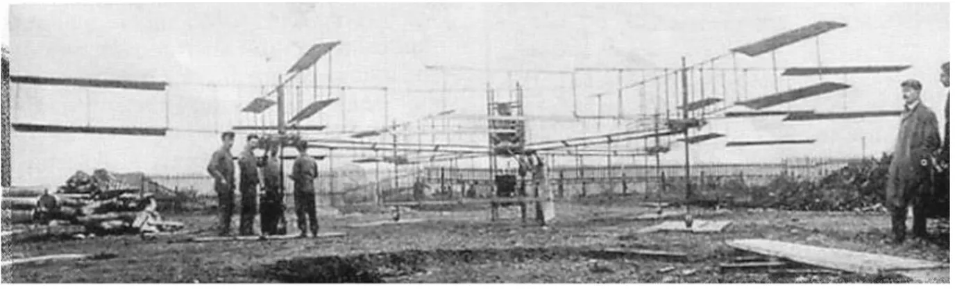
In 1920, a French engineer and helicopter designer Etienne Oehmichen designed several models and attempted to fly with them. L’hélicoptère no: 2 was the one of

4

his six designs and it had 8 propellers. L’hélicoptère no: 2’ s stability was significantly high. In Figure 1.4 L’hélicoptère no: 2 had took-off.

Figure 1.4 L’hélicoptère no: 2 [4]

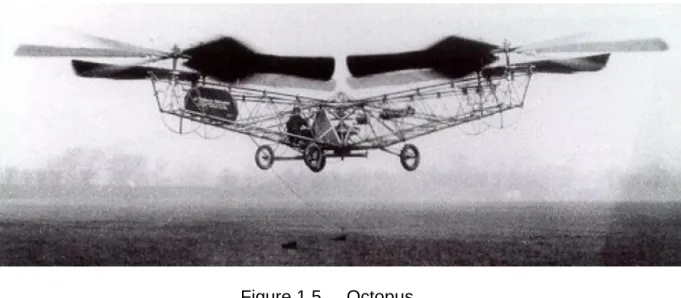
Another experiment was made in 1923 by a Russian engineer George de Bothezat with the vehicle named Octopus. It flew off the ground but it hadn’t acquired a successful flight. Nevertheless, it became an inspiration to nowadays quadrotor design. A photo of the Octopus was flying is shown in Figure1.5 [5].

Figure 1.5 Octopus

In both Oehmichen’s and Bothezat’s designs, the motors were driven by propellers perpendicular to the main rotors, that is why their designs weren’t considered as

5

successful quadrotor designs. 30 years later, in 1957, a new quadrotor designed and called Convertawings Model a Quadrotor by Marc Adman Kaplan (see Figure 1.6). The aircraft was designed to rotate four rotors with two motors and v-belts. Although the vehicle achieved great success as the first quadrotor capable of flying forward, had not been produced further due to low demand.

Figure 1.6 Convertawings Model a Quadrotor [6]

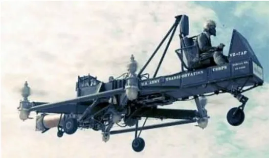
In 1958, the Curtiss-Wright company designed a quadrotor for American army, called Curtiss-Wright VZ-7 (see Figure 1.7), which was capable of vertical take-off and landing [7].

6

Figure 1.7 Curtiss-Wright VZ-7

These are the prototypes and designs that led the aviation to improve with new designs and experiments.

1.2.2 History of unmanned aerial vehicles

During and just after World War I the first pilotless aircraft was built. On 12 September 1917, the Hewitt-Sperry Automatic Airplane, known as the flying bomb was made its first flight. This flight had demonstrated the concept of an unmanned aircraft. Gyroscopes were invented by an American inventor Elmer Sperry from the Sperry Gyroscope Company and they were used for controlling and stabilizing. After the WW I, radio controlled drones started to be designed [8].

In World War II, Reginald Denny has built a first large-scale drone. He believed that low-cost RC (radio control) would be very useful for training anti-aircraft gunners, in 1935 he demonstrated a prototype target drone, the RP-1 to the US Army. In 1940, Denny and his partners continued to develop their design and signed a contract for their radio-controlled RP-4, which eventually became the Radioplane OQ-2 (see Figure 1.8) [9].

7

Figure 1.8 A Radioplane OQ-2 and its launcher [10]

1.3 Modern Era

The idea of Vertical Take-off and Landing (VTOL) has led the aviation industry to design various models. Since the beginning of the 2000s using high speed brushed direct current motors (BDCMs), integrated inertial measurement units (IMUs) and high-current li-on batteries has led the technology to improve and the resulted in mini and micro UAVs. In civilian respects, exploring mountainous terrain, forested areas, meteorological surveys, agricultural disinfection, data communication and in military respects, applications such as discovery and surveillance has come forward.

Recent quadrotor designs in the 21th century:

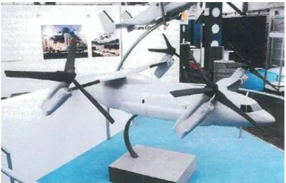
Bell Boeing Quad Tiltrotor (QTR) has four-rotor derivative of the Bell Boeing V-22 Osprey tiltrotor and it is developed by Boeing and Bell Helicopter (see Figure 1.9) [11].

8

Figure 1.9 Bell Boeing Quad Tiltrotor (QTR)

Anteos drone from Aermatica Spa is the first officially permitted rotary-wing radio-controlled drone which can fly in civil airspace (see Figure 1.10) [12].

Figure 1.10 Anteos A2-Mini

AeroQuad and ArduCopter are Arduino based open source software quadrotor projects (see Figure 1.11.a and b respectively).

9

Figure 1.11 AeroQuad [13] Figure 1.12 ArduCopter [14]

Parrot AR.Drone 2.0 designed by the French manufacturer Parrot SA. It has been designed for entertainment purposes (video gaming, augmented reality etc.) and it can be controlled via Smartphones through Wi-Fi (see Figure 1.12) [15] .

Figure 1.13 Parrot AR.Drone 2.0

Quadrotors have many advantages over conventional helicopters in terms of control and ease of installation. However, requirements of size and energy are the main disadvantages of the quadrotor. In terms of advantages of the quadrotors, they are simple in mechanics, their gyroscopic effect is low and they have high payload. In terms of disadvantages, they consume large amount of energy and their size and mass is large.

1.4 General Classification of Aircrafts

Generally, aircrafts can be classified under two categories: Lighter than air (LTA) and Heavier than air (HTA). In Figure 1.13 there is a general representation of aircrafts’ classification. In this classification including principle of flying and

10

propulsion mode. This aircraft classification states clearly, which category the quadrotors fall into.

Aircraft

Ornihopter Lighter than air

Power driven

Airship Non-Power

driven

Free Balloon Captive Balloon

Heavier than air

Power driven

Aeroplane Non-Power

driven

Glider Kite Rotorcraft

Figure 1.14 General aircraft classification [16]

1.5 Literature Review

There has been several researches and papers about UAVs and particularly about quadrotors. They are becoming very popular and their usage is highly extensive. From surveillance to gaming and in the near future they will become essential in some respects.

Bouabdallah [17] have designed a VTOL miniature flying robot (MFR) named OS4. They mathematically modelled and used both linear and nonlinear control techniques. To control OS4’s attitude they used Lyapunov theory. PID and LQ techniques were the second and the third controllers. Using these controllers they compared attitude control outcomes. Backstepping and sliding-mode controllers were used as the fourth and the fifth controller approaches, which are applied to control attitude. They finally augmented backstepping with integral and proposed this technique as a single tool to control design for attitude, altitude and position of OS4.

C. Balas [18] obtained nonlinear mathematical model and decoupled inputs of Dragonflyer X-Pro. He used PID and LQRto control the modelled quadrotor. His model comprises the controlling of the position and yaw angle of the quadrotor. In his work he used engineering and mathematical approaches in order to create a perfect model. Finally, he measured his model’s ability to track a given input trajectory. His way of modelling finally corresponds to stepping back from

11

mathematical approach and he achived optimal performances from his model which obtained with engineering approach.

Costa de Oliveira [19] mathematically modelled, experimentaly identified and controlled a small indoors quadrotor around hovering condition. Kalman Filter was used for state estimation and noise filtering. Other control techniques such as, PID, LQ, 𝐻∞ and µ-synthesis with DK-iteration were used. These techniques were compared with each other within reference tracking of flight trajectory and uncertainty of the model. He experimented that with 𝐻_∞ and µ-synthesis performs better results under uncertainity situations due to the robustness property.

Kim et al. [20] made a performance comparison of a quadrotor between LQR, LQR with gain scheduling, feedback linearization and sliding mode control techniques. Their experiment showed that LQR with gain scheduling has produced good performance with less effort of total control while sliding-mode control has returned fastest state regulation with the best performance.

Kıyak and Ermeydan [21] made fault tolerant control using improved PID controller with different motor fault cases in a quadrotor. He made a simulation by obtaining aircraft’s dynamic equations and modelling motor dynamics. In his simulation both linear and nonlinear models were compared within the scope of following trajectories. Control structure design was tested with different motor fault cases to state the robust control structure was successfully built.

Zulu and John [22] made a comparison between several control techniques (eg. PID,LQR, LQG, Sliding mode, feedback linearization, 𝐻∞ and fuzzy logic) applied to control the quadrotor. The conclusion of their work is a proposal of hybrid systems that can be considered as combination of more than one control technique’s advantages. Their work states the comparison of the quadrotor control techniques by the characteristics of these techniques and shows a table according to these features.

Karaahmetoğlu [23] made a trajectory control of a quadrotor using cascade control with state observer LGQ. He used PD, PID, LQR and LQG control and acquired better results with LQG control under various trajectory cases.

12

Fessi and Bouallégue, modelled a nonlinear dynamical quadrotor using Newton – Euler formalism. They designed LGQ control for attitude and altitude stabilization and acquired the weighting matrices by trial-errors. They showed their system’s effectiveness of their proposed flight stabilization by simulations [24].

After all these researches using Wind Shear as a turbulence in the quadrotor system was chosen. There is a lack of study about this type of turbulence effect on the quadrotors. As it was mentioned before, one of this thesis’ goals is to make a statement about the difference in terms of the effects of Gaussian white noise and Wind Shear turbulence on the quadrotor system.

1.6 Thesis Structure

The rest of this thesis is organized as follows.

In Chapter 2 system model was designed using Newton – Euler formalism. Some assumptions and generalities were made. Body and inertia frames, rotation matrix for transformation between the frames and finally equations of motions were derived and stated. For LQG control, a linearized model also stated. Through this chapter characteristics of the quadrotor can be seen clearly.

Chapter 3 shortly shows applied control techniques for attitude and altitude control of the quadrotor, which are PID and LQG. The controllers are verified using Simulink simulations and the results of these simulations can be found in Chapter 5.

Chapter 4 introduces new approach to disturbance usage on the quadrotor. A Wind Shear turbulence model was used and its effects are shown through body and inertial frames. Also Gaussian white noise applied to the system along with Wind Shear turbulence. System linearization explained and derived. Effects of the combination disturbances are showed in Chapter 5. Kalman Filter was used as state observer.

Chapter 5 discusses Gaussian white noise and turbulence effects on the quadrotor, PID and LQG techniques performances with simulation results.

Finally, Chapter 6 concludes by highlighting the objective and results of this work and proposes some improvements for the future work.

13 2. SYSTEM MODELLING

2.1 Quadrotor Concept and Generalities

A quadrotor consists of four rotors, each one placed at the end of a cross-like structure as shown in Figure 2.1. Each rotor consists of a two-blade propeller to an individually powered BLDCMs (Brushless DC Motors). The BLDCMs are different from the common BDCMs (Brushed DC Motors). In BDCM input voltage that applied to the armatures is done by a mechanical commutator (brush), due to this feature it suffers wear through its operation. As a result, BDCMs have shorter nominal life than BLDCMs [19].

Figure 2.1 Coordinate system of a Quadrotor [17]

Figure 2.1 also shows which direction of the rotors rotate. Rotor 1 and 3 rotates clockwise and rotor 2 and 4 rotates counter clockwise. Horizontal movement of the quadrotor is achieved by the generated torques from the rotors and vertical movement is achieved by the total thrust. Figure 2.2 shows an illustration of the quadrotor’s concept motion description, the arrow width is proportional to the propeller rotational speed.

14

Figure 2.2 Quadrotor’s motion [25] a) Yawing movement counter clockwise direction

b) Yawing movement clockwise direction c) Hovering or take-off

d) Rolling movement clockwise direction

e) Pitching movement counter clockwise direction f) Pitching movement clockwise direction

g) Descent or landing

h) Rolling movement counter clockwise direction

In order to design an efficient model of the quadrotor some assumptions were made:

 The structure is supposed to be rigid.

 The structure is supposed to be symmetrical.

 Origin of the both center of the gravity and the body fixed frame are assumed to coincide.

 The propellers are supposed to be rigid.

15

Quadrotor is a six DOF (degrees of freedom) flying vehicle, thus six variables (𝑥, 𝑦, 𝑧, 𝜙, 𝜃, 𝜓) are using to express its position in space. 𝑥, 𝑦 and 𝑧 represent the distance of the quadrotor’s center of mass along with the Earth fixed inertial frame. 𝜙, 𝜃 and 𝜓 are Euler angles and they represent the rotation of the quadrotor along x (between – 𝜋 and 𝜋), y (between –𝜋₂ and 𝜋₂), and z (between – 𝜋 and 𝜋) axes respectively. Further explanation and definitions about frames and Euler angles will be discussed in Body and Inertial Frames and in Rotational Matrix subsections.

2.2 Body and Inertia Frames

Firstly, the coordinate systems must be defined in order to be able to derive the model of the quadrotor. Figure 2.1 shows the Earth (inertial) frame with X, Y and Z conformity with the N, E, D (North, East, Down) and the body frame with 𝑥, 𝑦 and 𝑧 axes. The Earth (inertial) frame fixed on a specific place at ground level. Body frame is at the center of the quadrotor’s body with x-axis is pointing towards to the first propeller and y-axis is pointing towards to the second propeller. z – axis is pointing towards to the ground.

𝜁 = [ 𝑥 𝑦

𝑧] (2.1)

states the 3D position vector of the body frame with respect to the inertial frame.

𝑣 = [𝑥̇𝑦̇ 𝑧̇

] (2.2)

states the velocity vector of the body frame with respect to the inertial frame.

𝐴_𝑏 = [𝑥̈𝑦̈ 𝑧̈ ]

̇

(2.3)

states the acceleration vector of the quadrotor.

𝜔_𝑏 = [ 𝑝 𝑞

𝑟] (2.4)

16 2.3 Rotation Matrix

The rotation matrix R describes the orientation of the quadrotor from the body frame to the inertial frame. Quadrotor’s orientation is described using Euler Angles roll (phi, ϕ), pitch (theta, θ) and yaw (psi, ψ) representing rotations along with the X, Y and Z axes respectively. In this thesis, the order of rotation is in the sequence of yaw (ψ), pitch (θ) and roll (ϕ). Definitions of each Euler angles rotation matrices are given below: 𝑅₁(𝜙) = [ 1 0 0 0 𝑐𝑜𝑠𝜙 𝑠𝑖𝑛𝜙 0 −𝑠𝑖𝑛𝜙 𝑐𝑜𝑠𝜙] (2.5) 𝑅2(𝜃) = [ 𝑐𝑜𝑠𝜃 0 −𝑠𝑖𝑛𝜃 0 1 0 𝑠𝑖𝑛𝜃 0 𝑐𝑜𝑠𝜃 ] (2.6) 𝑅₃(𝜓) = [−𝑠𝑖𝑛𝜓 𝑐𝑜𝑠𝜓 0𝑐𝑜𝑠𝜓 𝑠𝑖𝑛𝜓 0 0 0 1 ] (2.7)

These three matrices are orthogonal matrices and the rotation matrix R is the matrix multiplication in the given sequence.

𝑅_𝑍𝑌𝑋 = 𝑅₁(𝜙)𝑅₂(𝜃)𝑅₃(𝜓) (2.8)

𝑅𝑍𝑌𝑋= [

𝑐𝑜𝑠𝜃𝑐𝑜𝑠𝜓 𝑐𝑜𝑠𝜃𝑠𝑖𝑛𝜓 −𝑠𝑖𝑛𝜃

𝑠𝑖𝑛𝜃𝑠𝑖𝑛𝜙𝑐𝑜𝑠𝜓 − 𝑠𝑖𝑛𝜓𝑐𝑜𝑠𝜙 𝑠𝑖𝑛𝜓𝑠𝑖𝑛𝜃𝑠𝑖𝑛𝜙 + 𝑐𝑜𝑠𝜓𝑐𝑜𝑠𝜙 𝑠𝑖𝑛𝜙𝑐𝑜𝑠𝜃

𝑠𝑖𝑛𝜃𝑐𝑜𝑠𝜙𝑐𝑜𝑠𝜓 𝑠𝑖𝑛𝜓𝑠𝑖𝑛𝜃𝑐𝑜𝑠𝜙 − 𝑐𝑜𝑠𝜓𝑠𝑖𝑛𝜙 𝑐𝑜𝑠𝜙𝑐𝑜𝑠𝜃] (2.9)

𝑅𝑍𝑌𝑋is also an orthogonal matrix due to this property 𝑅𝑍𝑌𝑋𝑇 = 𝑅𝑍𝑌𝑋. 2.4 Euler Angle Transformation

In flight control system, it is not possible to directly measure the Euler angles. However, the body angular velocities can be measured. The relationship between the body angular velocity vector [𝑝 𝑞 𝑟]𝑇 and the rate of change of the Euler angles, [𝜙̇ 𝜃̇ 𝜓̇]𝑇 can be determined by solving the Euler rates into the body coordinate frame [26].

17 [ 𝑝 𝑞 𝑟] = [ 𝜙̇ 0 0 ] + [ 1 0 0 0 𝑐𝑜𝑠𝜙 𝑠𝑖𝑛𝜙 0 −𝑠𝑖𝑛𝜙 𝑐𝑜𝑠𝜙] [ 0 𝜃̇ 0 ] + [ 1 0 0 0 𝑐𝑜𝑠𝜙 𝑠𝑖𝑛𝜙 0 −𝑠𝑖𝑛𝜙 𝑐𝑜𝑠𝜙] [ 𝑐𝑜𝑠𝜃 0 −𝑠𝑖𝑛𝜃 0 1 0 𝑠𝑖𝑛𝜃 0 𝑐𝑜𝑠𝜃 ] [ 0 0 𝜓̇] (2.9) [ 𝑝 𝑞 𝑟] = [ 1 0 −𝑠𝑖𝑛𝜃 0 𝑐𝑜𝑠𝜙 𝑠𝑖𝑛𝜙𝑐𝑜𝑠𝜃 0 −𝑠𝑖𝑛𝜙 𝑐𝑜𝑠𝜙𝑐𝑜𝑠𝜃] [ 𝜙̇ 𝜃̇ 𝜓̇ ] and [ 𝜙̇ 𝜃̇ 𝜓̇ ] = [ 1 𝑠𝑖𝑛𝜙𝑡𝑎𝑛𝜃 𝑐𝑜𝑠𝜙𝑡𝑎𝑛𝜃 0 𝑐𝑜𝑠𝜙 −𝑠𝑖𝑛𝜙 0 𝑠𝑖𝑛𝜙 𝑐𝑜𝑠𝜃⁄ 𝑐𝑜𝑠𝜙⁄_{𝑐𝑜𝑠𝜃} ] [ 𝑝 𝑞 𝑟](2.10) 𝐽−1 _{= [}1_{0 𝑐𝑜𝑠𝜙}0 _{𝑠𝑖𝑛𝜙𝑐𝑜𝑠𝜃}−𝑠𝑖𝑛𝜃 0 −𝑠𝑖𝑛𝜙 𝑐𝑜𝑠𝜙𝑐𝑜𝑠𝜃] (2.11)

𝐽−1 _{states the angular rotation matrix between body angular vector and the rate of} Euler angles change vector.

Around the hover position, considering small angles where 𝑐𝑜𝑠𝜙 = 1, 𝑐𝑜𝑠𝜃 = 1and 𝑠𝑖𝑛𝜙 = 𝑠𝑖𝑛𝜃 = 0 then 𝐽−1_{can be simplified to an identity matrix 𝐼}

[3𝑥3].

2.5 Modelling with Newton-Euler Formalism

There are two different methods for deriving equations of motions, which are Lagrangian equation and Newton – Euler formalism. In this thesis, Newton – Euler formalism is used.

The dynamics of a rigid body under external forces applied to the center of mass and expressed in the body frame are in Newton-Euler formalism [17]:

[𝑚𝐼[3𝑥3] 0 0 𝐼] [ 𝑉𝑏 ̇ 𝜔𝑏̇ ] + [ 𝜔 × 𝑚𝑉_𝑏 𝜔 × 𝐼𝜔𝑏] = [ 𝐹_𝑏 τ_𝑏] (2.12) Thus, 𝐹𝑏= 𝑚𝐼[3×3]𝑉𝑏̇ + 𝑚𝜔 × 𝑉𝑏 (2.13) 𝜏_𝑏 = 𝐼𝜔̇ + 𝜔 × 𝐼𝜔_𝑏 (2.14)

18 𝐼⃗ = [

𝐼𝑥𝑥 𝐼𝑥𝑦 𝐼𝑥𝑧 𝐼𝑦𝑥 𝐼𝑦𝑦 𝐼𝑦𝑧 𝐼𝑧𝑥 𝐼𝑧𝑦 𝐼𝑧𝑧

] and since an assumption made about the structure being symmetrical, thus 𝐼⃗ become diagonal:

𝐼⃗ = [ 𝐼_𝑥 0 0 0 𝐼𝑦 0 0 0 𝐼𝑧 ] (2.15) 𝐼_𝑥= 𝐼_𝑦 = 2(𝑚_𝑟𝑙2_{) +}2 5𝑚𝑠𝑟2 (2.16) 𝐼_𝑧= ∑4𝑗=1(𝑚𝑟𝑙2) +₅2𝑚𝑠𝑟2 (2.17)

2.5.1 Aerodynamic moments and forces

The quadrotor is controlled by varying four rotor’s speed independently. Figure 2.1 shows how thrust and torques by each rotor produced. Four control inputs were used for modelling the quadrotor:

1) The total thrust: 𝑈₁ = 𝐹₁+ 𝐹₂ + 𝐹₃+ 𝐹₄ = 𝑏(𝜔₁+ 𝜔₂+ 𝜔₃+ 𝜔₄) (2.18)

2) Rolling moment: 𝑈2 = 𝑙(𝐹2− 𝐹4) = 𝑏𝑙(𝜔22− 𝜔42) (2.19)

3) Pitching moment: 𝑈3 = 𝑙(𝐹1− 𝐹3) = 𝑏𝑙(𝜔12− 𝜔32) (2.20)

4) Yawing moment: 𝑈4 = 𝑑_𝑏(𝐹1− 𝐹2+ 𝐹3 − 𝐹4) = 𝑑(𝜔12− 𝜔22+ 𝜔32− 𝜔42) (2.21) Where,

𝐹𝑖 =1₂𝜌𝐴𝐶𝑇𝑟2𝜔𝑖2 = 𝑏𝜔𝑖2 (2.20)

states the thrust force produced by the 𝑖𝑡ℎ _rotor

𝑀𝑖 =1₂𝜌𝐴𝐶𝐷𝑟2𝜔𝑖2 = 𝑑𝜔𝑖2 (2.21)

states the torque moment produced by the 𝑖𝑡ℎ _rotor 𝜌 air density (kg/m3₎

A area of the propeller disc (m2₎ CT non-dimensional thrust coefficient

19 CD non-dimensional drag torque coefficient

r radius of the propeller (m)

𝜔_𝑖 angular velocity of the 𝑖𝑡ℎ _{rotor (rad/sec)}

b thrust constant

d torque constant

𝑙 lever length of each of the arms

𝑚𝑟 mass of propeller

𝑚_𝑠 mass of sphere

2.5.2 Gyroscopic effect

The gyroscopic moment of a rotor is a physical effect in which gyroscopic torques or moments attempt to align the spin axis of the rotor along with the inertial z-axis [27]. The gyroscopic effect from the rotation of the propellers:

𝜏_𝑥′ _{= 𝐽}

𝑟𝜔𝑦(𝜔1− 𝜔2+ 𝜔3− 𝜔4) (2.22)

𝜏_𝑦′ _{= 𝐽}

𝑟𝜔𝑥(−𝜔1+ 𝜔2− 𝜔3+ 𝜔4) (2.23)

2.5.3 Gravitational force

Earth’s gravitational field causes an interaction with the weight of the quadrotor. Gravitational force acting on the inertial frame:

𝐹𝑔 = [ 0 0

𝑚𝑔] (2.24)

2.6 Equations of Motion

Total force equation acting on the quadrotor’s body frame:

𝑚 [𝑦̈𝑥̈ 𝑧̈ ] = 𝑈₁[ 𝑐𝑜𝑠𝜙𝑐𝑜𝑠𝜓𝑠𝑖𝑛𝜃 + 𝑠𝑖𝑛𝜙𝑠𝑖𝑛𝜓 𝑐𝑜𝑠𝜙𝑠𝑖𝑛𝜓𝑠𝑖𝑛𝜃 − 𝑠𝑖𝑛𝜙𝑐𝑜𝑠𝜓 𝑐𝑜𝑠𝜙𝑐𝑜𝑠𝜃 ] − [ 0 0 𝑚𝑔] (2.24)

20

Total moment equation acting on the quadrotor’s body frame:

[ 𝐼_𝑥𝜙̈ 𝐼_𝑦𝜃̈ 𝐼𝑧𝜓̈ ] = [ (𝐼_𝑦− 𝐼_𝑧)𝜃̇𝜓̇ (𝐼_𝑧− 𝐼_𝑥)𝜙̇𝜓̇ (𝐼𝑥− 𝐼𝑦)𝜙̇𝜃̇ ] + 𝑈₄[_−𝐽𝐽𝑟_𝑟𝜃̇_𝜙̇ 0 ] + [ 𝑈2 𝑈₃ 𝑈4 ] (2.25)

List of force and moment equations:

𝑥̈ =𝑈1 𝑚(𝑐𝑜𝑠𝜙𝑐𝑜𝑠𝜓𝑠𝑖𝑛𝜃 + 𝑠𝑖𝑛𝜙𝑠𝑖𝑛𝜓) 𝑦̈ =𝑈1 𝑚(𝑐𝑜𝑠𝜙𝑠𝑖𝑛𝜓𝑠𝑖𝑛𝜃 − 𝑠𝑖𝑛𝜙𝑐𝑜𝑠𝜓) 𝑧̈ =𝑈1 𝑚(𝑐𝑜𝑠𝜙𝑐𝑜𝑠𝜃) − 𝑔 𝜙̈ =(𝐼𝑦−𝐼𝑧) 𝐼𝑥 𝜃̇𝜓̇ + 𝐽𝑟 𝐼𝑥𝜃̇𝑈4 + 1 𝐼𝑥𝑈2 (2.26) 𝜃̈ =(𝐼𝑧−𝐼𝑥) 𝐼𝑦 𝜙̇𝜓̇ − 𝐽𝑟 𝐼𝑦𝜙̇𝑈4+ 1 𝐼𝑦𝑈3 𝜓̈ =(𝐼𝑥−𝐼𝑦) 𝐼𝑧 𝜙̇𝜃̇ + 1 𝐼𝑧𝑈4 2.7 Simulink Model for Quadrotor

From Figures 2.3 to 2.6 Simulink model of the quadrotor can be seen step by step. In Figure 2.3 the top view of the quadrotor is shown. For the simplicity, all desired signals generated by a Signal Builder. PID control for the attitude and altitude of the quadrotor is done in the PID Control block. Wind Turbulence consists of Wind Shear turbulence model, which can be found in Simulink under Aerospace Blockset.

21

Figure 2.3 Quadrotor’s top view of the Simulink model

Figure 2.4 shows all the PID control blocks for attitude and altitude control. Desired signals and the calculated states form the Quadrotor System is subtracted, so an error signal for every control is calculated. All these signals united in a bus by using a Bus Creator and for the subtraction they all separated by using a Bus Selector. In Chapter 3, further details about the PID structure for the attitude and altitude control of the quadrotor can be found.

22

Figure 2.4 PID control blocks for the attitude and the altitude control of the quadrotor

Figure 2.5 shows quadrotor model designed with respect to the Newton – Euler formalism. Torques and Thrust block generates control signals, which are 𝑈1, 𝑈2, 𝑈3 and 𝑈4. These control signals directly goes to the main calculation block, which named 6DOF. The 6DOF block calculates all the states with respect to the given inputs, in this case step signals.

23

Figure 2.5 Designed quadrotor model with 6DOF block

In Figure 2.6 inside of the 6DOF block is shown. All calculations; Euler angles, body angular velocity, inertial position, derivative of the body angular velocities, body velocities, inertial velocities and rotation matrix (in the figure stated as DCM matrix) are done.

24 2.8 Linearized Quadrotor

In order to use linear control techniques on a nonlinear system to control attitude and altitude, the system must be linearized at a feasible point. Further details and linearization point explanations will be discussed in Chapter 3. For the sake of clarity, a block diagram of the linearized system process can be seen in Figure 2.7.

Figure 2.7 Linearized system process

In this figure, U states control signals, which are 𝑈₁, 𝑈₂, 𝑈₃ and 𝑈₄. Quadrotor block calculates the states (𝑥, 𝑦, 𝑧, 𝜙, 𝜃, 𝜓, 𝑥,̇ 𝑦,̇ 𝑧,̇ 𝜙,̇ 𝜃̇ and 𝜓̇) and the outputs ( 𝜙, 𝜃, 𝜓 and 𝑧). All these inputs goes to the linearization block and they get linearized at the equilibrium flight point. After the linearization process is completed, linear control techniques applied to the linearized system. Further details about the linearization process and the applied linear control can be found in Chapter 3.

25 3. SYSTEM AND CONTROL DESIGN

After identification of the quadrotor is done, the control design of the quadrotor can be proceeded. Due to the instability and nonlinearity of the quadrotor, designing an efficient and a reliable control is needed. For controlling the quadrotor, PID (Proportional Integral Derivative) and LQR (Linear Quadratic Regulator) / LQG (Linear Quadratic Gaussian) techniques is used.

3.1 PID Control

PID (proportional integral derivative) is a closed loop control and it tries to achieve the measured result closer to the desired result by adjusting the input. This control chosen over PD (Proportional Derivative) because of the steady state error. PID can eliminate the steady state error owing to its integral feature. PID control used for achieving stability of the quadrotor and has control parameters namely, 𝑘𝑝 for proportional gain, 𝑘𝑖 for integral gain and finally 𝑘𝑑for derivative gain. By changing these gains system can become more stable, transient response and steady state accurate. General representation of a PID control showed in Figure 3.1.

Figure 3.1 General representation of PID controller

26 Table 3.1 Effects of PID gains

Response Rise Time Overshoot Settling Time Steady State Error

𝑘_𝑝 Decreases Increases Small change Decreases

𝑘𝑖 Decreases Increases Increases Eliminate

𝑘𝑑 Small change Decreases Decreases No change

The derived PID control law is:

𝑢(𝑡) = 𝑘𝑝𝑒(𝑡) + 𝑘𝑖∫ 𝑒(𝑣)𝑑𝑣₀𝑡 + 𝑘𝑑𝑑𝑒(𝑡)_𝑑𝑡 (3.1) Where,

𝑢(𝑡) states the controlled variable, 𝑒 is the error signal, which is the difference between desired value and measured value.

There are two main disadvantages in the general PID controller [21]:

1) Since the derivative effect is calculated using error signal of the system, the output of the derivative will be an impulse function when a step input is applied to the system. This can cause the system moved away from the linear zone by saturating the actuators.

2) Combination of actuators’ saturation and effect of the integral can cause a nonlinear effect. This will lead a decrease in controller’s performance. Another issue is integral winding, which occurs when the integral value is large and the sign of the error signal changes it takes time to change the sign of the integral. To prevent this situation, the integral effect should be limited to minimum and maximum values.

In figure 3.2 a new approach used in PID controller to prevent these undesired situations [28].

27

Figure 3.2 New approach of PID controller

In this thesis four PID controller designed to control roll, pitch, yaw and altitude (z). Also in Figure 3.2 roll PID control scheme can be seen. The other PID controls of pitch, yaw and altitude have the same structure. Figures 3.3, 3,4 and 3-5 shows respectively.

28

Figure 3.4 Yaw PID control

Figure 3.5 Altitude PID control

29 Table 3.2 PID control gains

Proportional Gain Integral Gain Derivative Gain

Roll Control 0.8 0.0002124 0.1126

Pitch Control 1.2 0.0013 0.213

Yaw Control 1 0.00001024 0.17803

Altitude Control 100 0.286 12

Figure 5.1 in Chapter 5, shows response of the quadrotor system to the applied step signal as desired roll, pitch, yaw and z. Also, this figure shows that wind shear effect is eliminated by PID control. Index 1 for this graph indicates desired values and index 2 for this graph indicates quadrotor’s response.

Figure 5.2 in Chapter 5, shows wind shear turbulence block’s output when 6 meters of height and Direct Cosine Matrix (DCM), which is equation 2.8 from Chapter 2 applied. Details about wind shear will be given in Chapter 4.

In Figure 5.3 from Chapter 5, Wind Shear effect on the inertial frame can be seen.

It is clear that quadrotor model with PID control can eliminate the wind shear turbulence effect from the quadrotor system.

3.2 Linear Quadratic Regulator (LQR) and Linear Quadratic Gaussian (LQG)

LQR is a linear control technique for multiple input multiple input (MIMO) systems and it provides a practical feedback gain. To use LQR we need to characterize the model with transfer matrices instead of transfer functions. Further information about this technique can be found in Lewis and Stevens [28, 29].

30

𝑥⃗̇(𝑡) = 𝐴𝑥⃗(𝑡) + 𝐵𝑢⃗⃗(𝑡) (3.2)

𝑦(𝑡) = 𝐶𝑥⃗(𝑡) + 𝐷𝑢⃗⃗(𝑡) (3.3)

Where, 𝐴 is the system matrix, 𝐵 is the input matrix, 𝐶 is the output matrix and 𝐷 is the feedback through matrix. Also 𝑥⃗ is the state vector, 𝑦⃗ is the output vector and 𝑢⃗⃗ is the input vector.

𝐽 is the quadratic cost function which will be minimized by 𝑄, cost of the state (a positive semi-definite matrix; 𝑄 = 𝑄𝑇_{) and 𝑅 cost of the actuators (a positive definite} matrix; 𝑅 = 𝑅𝑇_):

𝐽 =1₂∫ (𝑥⃗∞ 𝑇_{𝑄𝑥⃗ + 𝑢⃗⃗𝑅𝑢⃗⃗)𝑑𝑡}

0 (3.4)

The gain matrix 𝐾 is:

𝐾 = 𝑅−1_𝐵𝑇_{𝑆 (3.5)}

Where S is the Algebraic Ricatti Solution:

0 = 𝐴𝑇_{𝑆 + 𝑆𝐴 − 𝑆𝐵𝑅}−1_𝐵𝑇_{𝑆 + 𝑄 (3.6)}

𝑄 and 𝑅 matrices are very important and the meanings of their values to the system are [29]:

 If 𝑄 = 𝑅, regulation speed and the energy spend for control is equally important

 If 𝑄 > 𝑅, regulation speed is more important than the energy spend for control. This means big valuable control signals were chosen to acquire fast regulation.

 If 𝑄 < 𝑅, the energy spend for control is more important than regulation speed. This means using less control to spend less energy for control were chosen. On the other hand, regulation will be done slowly and it will take time.

The quadrotor model described in Chapter 2 is a nonlinear model, therefore the model needs to be linearized to apply LQ regulator. Linearization point is chosen at

31

the equilibrium flight point, which means moments are zero (rolling, pitching and yawing) and total thrust is equal to the gravitational force.

From Chapter 2 equation 2.18 total thrust 𝑈₁ = 𝐹₁+ 𝐹₂+ 𝐹₃+ 𝐹₄ = 𝑏(𝜔₁+ 𝜔₂+ 𝜔3+ 𝜔4) and it equals to 𝐹𝑔 = 𝑚𝑔 therefore all rotor’s angular speeds are equal. Recall moment equations from Chapter 2 (equations from 2.19 to 2.21), they all contains difference of the squared rotor speed. That is why all of the moments are equal to zero.

Another important point for linearization is that since there will be any moment then Euler angles are equal to zero. For the Wind Shear effect only 𝑧 position in the inertial frame is chosen 6 meters, 𝑥 and 𝑦 positions are equal to zero as well. First, we need to define our system’s state, input and output vectors. These vectors can be found below respectively.

𝑥⃗ = [𝑥 𝑦 𝑧 𝜙 𝜃 𝜓 𝑥̇ 𝑦̇ 𝑧̇ 𝜙̇ 𝜃̇𝜓̇]𝑇 _(3.7)

𝑦⃗ = [𝜙 𝜃 𝜓 𝑧]𝑇 _(3.8)

𝑢⃗⃗ = [𝑈1 𝑈2 𝑈3 𝑈4]𝑇 _(3.9)

For the sake of notation simplicity, we shall drop ⃗⃗⃗⃗ from now on.

As mentioned before we will linearize this nonlinear system around the equilibrium flight point, so the linearization points in 𝑥 the state vector and 𝑢 the input vector are given below:

𝑥 = [0 0 6 0 0 0 0 0 0 0 0 0]𝑇 _{and 𝑢 = [𝑚𝑔 0 0 0]}𝑇 _(3.10) Using these linearization points and equations 2.6 from Chapter 2 our 𝐴, 𝐵, 𝐶 𝑎𝑛𝑑 𝐷 matrices will become:

32 𝐴 = [ 0 0 0 0 0 00 0 0 0 0 0 0 00 0 0 0 0 0 1 00 1 0 0 0 0 0 00 0 0 0 0 0 0 00 0 1 0 0 1 0 00 0 0 0 0 0 0 00 0 0 0 0 0 0 00 0 0 0 0 0 0 00 0 0 0 0 0 0 00 0 0 0 0 0 1 00 1 0 0 0 0 0 00 0 0 0 0 0 0 00 0 0 0 0 0 0 00 0 0 0 0 0 0 00 0 0 0 0 0 0 00 0 0 0 0 0 0 0 (𝐼𝑦− 𝐼𝑧) 𝐼_𝑥 𝜓̇ (𝐼𝑦 − 𝐼𝑧) 𝐼𝑥 𝜃̇ 0 (𝐼𝑧− 𝐼𝑥) 𝐼_𝑦 𝜓̇ 0 (𝐼𝑥− 𝐼𝑦) 𝐼𝑧 𝜃̇ 0 (𝐼𝑧− 𝐼𝑥) 𝐼_𝑦 𝜙̇ (𝐼_𝑥− 𝐼_𝑦) 𝐼𝑧 𝜙̇ 0 ]_12𝑥12 𝐵 = [ 0 0 00 0 0 00 0 0 00 0 0 00 0 0 00 0 0 00 (𝑐𝑜𝑠𝜙𝑠𝑖𝑛𝜃𝑐𝑜𝑠𝜓 + 𝑠𝑖𝑛𝜙𝑠𝑖𝑛𝜓) 𝑚 (𝑐𝑜𝑠𝜙𝑠𝑖𝑛𝜃𝑠𝑖𝑛𝜓 − 𝑠𝑖𝑛𝜙𝑐𝑜𝑠𝜓) 𝑚 0 0 (1 − (𝑐𝑜𝑠𝜙𝑠𝑖𝑛𝜃)) 𝑚 0 0 1 𝐼_𝑥 0 0 00 0 0 0 0 0 0 00 1 𝐼𝑦 0 0 1 𝐼𝑧 ]_12𝑥4 𝐶 = [ 0 0 0 1 0 0 0 0 0 0 1 0 0 0 0 0 0 0 0 0 0 0 0 0 0 0 0 0 0 1 0 0 1 0 0 0 0 0 0 0 0 01 0 0 0 0 0 ] 4𝑥12 𝐷 = [ 0 0 00 0 0 00 0 0 00 0 0 00 0 0 00 0 0 00 0 0 00 0 0 0 0 0 0 00 0 0 00 0 0 0 0 0 0 00]12𝑥4

33

The constants, which are used to calculate the matrices as follows:

Table 3.3 Quadrotor constants

Constants Value Unit

𝐼𝑥 7.5𝑥10−3 𝑘𝑔 𝑚2

𝐼_𝑦 7.5𝑥10−3 _{𝑘𝑔 𝑚}2

𝐼_𝑧 1.3𝑥10−2 _{𝑘𝑔 𝑚}2

Results of the state matrices after using these constants:

𝐴 = [ 0 0 0 0 0 00 0 0 0 0 0 0 00 0 0 0 0 0 1 00 1 0 0 0 0 0 00 0 0 0 0 0 0 00 0 1 0 0 1 0 00 0 0 0 0 0 0 0 0 0 0 0 0 0 0 00 0 0 0 0 0 0 0 0 0 0 0 0 0 0 00 0 0 0 0 0 1 0 0 1 0 0 0 0 0 00 0 0 0 0 0 0 00 0 0 0 0 0 0 00 0 0 0 0 0 0 00 0 0 0 0 0 0 00 0 0 0 0 0 0 00 0 0 0 0 0 0 00 0]12𝑥12 𝐵 = [ 0 0 00 0 0 00 0 0 00 0 0 00 0 0 00 0 0 00 1.5385 0 00 0 0 0 133.3333 0 0 00 0 0 00 0 0 00 133.3333 0 0 76.9231]12𝑥4

Due to the assumptions LQR makes, that all states are known and whole state is available to control at all times, that is simply unrealistic not only there will always be measurement noise interfering the system but also this technique become

34

impractical when some states cannot be measured directly. When some of the states cannot be measured, state prediction technique always can be used. In order to predict all the states in the system through measured ones we need to use LQG.

LQG and LQR have almost the same representation and mechanism except noises included, which are 𝑤 and 𝑣. These noises mean measurement noise and process noise respectively.

Thus, LQG state space representation as follows:

𝑥̇ = 𝐴𝑥 + 𝐵𝑢 + 𝑤 (3.11)

𝑦 = 𝐶𝑥 + 𝑣 (3.12)

For the simplicity, it is assumed that these noises are zero mean uncorrelated white Gaussian noises.

To use LQG control in a system one must follow these steps. Firstly, 𝑥̂ estimation must be calculated for the full state of 𝑥 using measurements and secondly, LQR controller must be apply to the system and it should use the estimation 𝑥̂ in place of the actual (presently non-measured) state of 𝑥.

This whole process led us to use Kalman Filter as a state observer in the system to estimate 𝑥̂ . Further details and expressions about Kalman Filter can be found in Chapter 4.

35 4.TURBULENCE AND NOISE FILTERING

The goal of this thesis is to state the difference of the turbulence and the Gaussian white noise effects on the system. In this chapter Kalman Filter employed as a state observer. Through Kalman Fillter these disturbances will be extracted from the quadrotor system.

4.1 Wind Shear Turbulence Model

Wind shear is a change in wind speed and/or direction over a short distance and it is a non – Gaussian turbulence. It can occur either horizontally or vertically and is most often associated with strong temperature inversions or density gradients. Wind shear can occur at high or low altitude and near buildings [30] and these situations are most likely to happen to a quadrotor in reality. According to these reasons, wind shear turbulence model was chosen to study and in this thesis only low altitude (at 6 meters) will be discussed.

In Figure 4.1 Matlab&Simulink’s wind shear model can be seen.

Figure 4.1 Wind shear model [31]

This model uses height in meters and Direct Cosine Matrix (DCM) and calculates the mean wind speed in the Earth axis and the output is the mean wind speed in the body axis. The equation for the mean wind speed in the Earth axis is:

𝑢_𝑊 = 𝑊₆ln( ℎ 𝑧0)

ln(20_𝑧0) (4.1)

Where ℎ is 3 m < ℎ < 304.8 m, 𝑢_𝑊 is the mean wind speed, 𝑊₆ is the measured wind speed at an altitude of 6 meters, ℎ is the altitude and 𝑧₀ is a constant equal to 0.045 meters for category C flight phases and 0.6 meters for all other flight phases [31].

36 4.2 Kalman Filter

Large amount of literature on this filtering technique is available. A detailed derivation and study on this topic can be found in Optimal Filtering by Anderson and Moore [32]. To explain briefly, the Kalman Filter is a state observer for the stochastic cases, where Gaussian zero-mean noise added to the both inputs and outputs. Kalman Filter scheme, which is shown in Figure 4.2.

Figure 4.2 Kalman state-observer scheme [31]

The filter’s linear model is:

𝑥̇ = 𝐴𝑥 + 𝐵𝑢 + 𝑤 (4.2)

𝑦 = 𝐶𝑥 + 𝑣 (4.3)

Kalman Filter uses system’s inputs and outputs, then generates an optimal estimate of 𝑥̂ and 𝑦̂ for all states whereas eliminating the noise effects.

𝑥̂̇ = 𝐴𝑥̂ + 𝐵𝑢 (4.4)

𝑦̂ = 𝐶𝑥̂ (4.5)

Where 𝑤 is in the LQG, white process noise and 𝑣 is as in the LQG, white measurement noise.

In Figure 4.3 mathematical formulation of Kalman Filter illustrated. Kalman Filter executes 6 steps over and over again with a sample time between the executions [33].

37

Figure 4.3 Mathematical Formulation of Kalman Filter

State prediction occurs when Kalman Filter predicts the next state using the current state and control signals. A block diagram for Kalman Filter is in figure 4.4.

Figure 4.4 Kalman state observer Mathworks’ block diagram [34]

Kalman filter as state observer is used when some of the states cannot measured. In this thesis Kalman Filter employed as a state observer along with the LQR, which is a LGQ control can be found in Figure 4.5.

38

Figure 4.5 Kalman Filter as state observer and LQR

When using Kalman Filter as state observer state space representation becomes:

𝑥̂̇ = 𝐴𝑥̂ + 𝐵𝑢 + 𝐿(𝑦 − 𝐶𝑥̂) (4.6)

and the necessary calculations for the state observer:

𝐿 = 𝑃𝐶𝑇_𝑅−1 _(4.7)

0 = 𝐴𝑃 + 𝑃𝐴𝑇_{− 𝑃𝐶}𝑇_𝑅−1_{𝐶𝑃 + 𝑄}𝑌 _(4.8)

When 𝑃 ≥ 0,

𝑄 = 𝐸(𝑤𝑤𝑇_{) and 𝑅 = 𝐸(𝑣𝑣}𝑇_{) (4.9)}

The Ricatti equation has its origin in the minimization of the cost functional[35].

𝐽[𝑥̂(∙)] = ∫ [(𝑥̂ − 𝑥)(𝑥̂ − 𝑥)0 𝑇_]𝑑𝑡

−∞ (4.10)

Another important case to use Kalman Filter as a state observer in LQG are that, the state matrices must be both controllable and observable. Both for controllability 𝒞 = [𝐵 𝐴𝐵 𝐴2_{𝐵 … 𝐴}𝑛−1_{𝐵] and observability 𝒪 = [𝐶 𝐶𝐴 𝐶𝐴}2_{… 𝐶𝐴}𝑛−1_{] must be full} rank.

𝑄 and 𝑅 matrices in both Kalman observer and LQR control must be chosen wisely. Otherwise, the regulation takes time to reach zero error and also Kalman filter cannot estimate the states accurately.

39

5. SIMULATION RESULTS AND DISCUSSION

5.1 PID Control Results

PID control for attitude and altitude performs great results under wind turbulence, which is wind shear in this thesis. Figure 5.1 shows quadrotor system’s response to the step signal. PID control for the attitude and altitude control rises with zero overshoot and settles around 5.5 seconds for all controls.

Figure 5.1 Response of the quadrotor system with PID control

As it could be seen throughout this thesis, the mentioned goals of this work are achieved. Wind shear can be eliminated by PID control and with LQG controller (LQR and Kalman state observer) both Wind Shear and Gaussian white noise can be eliminated.

Figure 5.2 shows Wind Shear turbulence model’s output, which is a wind velocity in the body axis.

40

Figure 5.2 Wind Shear response

In Figure 5.3 without Wind Shear effect on the body velocity of the quadrotor can be seen. To see the effect of the Wind Shear on the quadrotor Wind Shear added body velocity is shown in Figure 5.4.

41

Figure 5.3 Quadrotor’s body velocity without Wind Shear effect

Figure 5.4 Wind Shear effect on quadrotor’s body velocity

In Figure 5.5Wind Shear’s output wind velocity applied to the inertial positions (x, y and z axis) can be seen. Recall that desired signals are step signals but the Wind Shear disturbs the step signal.

42

Figure 5.5 Wind shear effect on quadrotor’s inertial frame

It is clear from the Figure 5.1, PID control for the given gains can eliminate the Wind Shear effect form the inertial frame. The constructed quadrotor model is stable and controllable under the wind turbulence.

5.2 LQG Control Results

Expectation is LQG regulates and estimates all the states and after these processes all states should approach to zero. The amount of time spent for these processes shows the controller’s performance.

43

Figure 5.6 Linearized quadrotor system’s step response

Figure 5.6 shows LQG control’s estimation and reference tracking result of an applied reference step signal r. Another expression to this figure is systems step response to the reference step signal.

44

Figure 5.7 LQG controller’s output without Gaussian white noise

LQG’s regulation and estimation performance without Gaussian white noise can be seen in Figure 5.7. All states approaches to zero after approximately 12 seconds.

Figure 5.8 LQG controller’s output with Gaussian white noise

Gaussian white noise added system’s response can be seen in Figure 5.8. Again LQR’s regulation and estimation is expected, all states reaches to zero after approximately 12 seconds.

45

In Figure 5.9 shows closed loop state feedback control response to initial conditions, which are equals to 1. Also in this figure, wind shear effect can be seen clearly on the output. In spite of the wind shear effect on the system LQG estimates and regulates successfully.

Figure 5.9 Closed loop controller’s response to the initial conditions

From these simulation results, one can say that linear control techniques successfully applied to the linearized system. System’s linearization at the linearization point is done correctly. Also results are promising in the way that the system can regulate the states and estimate them close to the actual values in spite of the disturbances. Another point to state, Gaussian white noise and Wind Shear are effecting the system differently. From figures 5.8 and 5.9 effects of these disturbances can be seen.

46 6. CONCLUSION AND FUTURE WORK

Throughout the applied control techniques, the proposed thesis goals are achieved. The quadrotor’s principal flight dynamics were investigated and a nonlinear model was derived using Newton – Euler formalism. According to the assumptions system’s parameters such as moments of inertia are derived. Performance of the PID control under wind shear turbulence examined. Relatively more difficult disturbance, Gaussian white noise added to the quadrotor system along with the Wind Shear and these disturbances eliminated in the linearized model using LQG control. For linearization, an equilibrium flight operating point was chosen and LQG performed on this point successfully. Kalman Filter was employed as a state observer to estimate unmeasurable states. Due to avoid sensor modelling and sensor calibration artifacts, the Kalman observer, namely LQG structure, used in the

system. Owing to LQG’s estimation feature the designed control system

successfully eliminated the disturbances. Wind shear is not a Gaussian disturbance, it is a statistics of velocities differences between points with some distance apart. The results shows that, Wind Shear and Gaussian white noise had different effects on the quadrotor system and the proposed control approach successfully rejected these disturbances.

However, in order to make this model close to the reality as possible as sensors can be added to the model. In this study, there are no robustness investigated. In real life robustness is a real issue and this model can be improved employing 𝐻_∞ control. Another suggestion to improve the current study is LQG control can be applied to velocities along with the positions. This way, a cascaded control structure can be achieved and even better results can be obtained. Also, the designed model can be built and the performance of these applied control techniques can be investigated not only in simulation but also in real life outside conditions.

47 REFERENCES

[1] “Hazerfen Ahmet Çelebi.”

[2] "Helical Air Screw," https://en.wikipedia.org/wiki/Propeller_(aeronautics). [3] "The Pioneers / Aviation and Aeromodelling-interdependent Evolutions and

Histories," http://www.ctie.monash.edu.au/hargrave/breguet.html.

[4] S. A. Raza, and W. Gueaieb, "Intelligent flight control of an autonomous quadrotor," Motion Control: InTech, 2010.

[5] “Flying Octopus.”

[6] "Convertawings Model A,"

http://www.aviastar.org/helicopters_eng/convertawings.php. [7] “Curtiss-Wright VZ-7.”

[8] L. Pearson, “Developing the flying bomb,” Naval Aviation in World War I, pp. 70-73, 1969.

[9] http://www.ctie.monash.edu.au/hargrave/dennyplane.html.

[10] “Radioplane OQ-2.”

[11] "Anonim, Bell QTR Quad Tiltrotor," http://www.aviastar.org/helicopterseng /bell_qtr.php.

[12] G. Mortimer, Anteos APR. "Aermatica," http://www.suasnews.com. [13] "AEROQUAD," http://aeroquad.com/content.php.

[14] "The ArduCopter," https://code.google.com/p/arducopter/.

[15] A. Arnold. "The Parrot AR.Drone," http://the-parrot-ardrone.com/. [16] “Aircraft Classification.”

[17] S. Bouabdallah, “Design and control of quadrotors with application to autonomous flying,” 2007.

[18] C. Balas, “Modelling and linear control of a quadrotor,” 2007.

[19] M. de Oliveira, “Modeling, identification and control of a quadrotor aircraft,”

Czech Technical University, Prague, 2011.

[20] T. S. Kim, K. Stol, and V. Kecman, "Control of 3 DOF quadrotor model,"

Robot Motion and Control 2007, pp. 29-38: Springer, 2007.

[21] E. Kıyak, and A. Ermeydan, “Bir döner kanata arıza toleranslı uçuş kontrol sistemi tasarımı,” Journal of the Faculty of Engineering and Architecture of

Gazi University, vol. 32, no. 1, pp. 21-34, 2017.

[22] A. Zulu, and S. John, “A review of control algorithms for autonomous quadrotors,” arXiv preprint arXiv:1602.02622, 2016.

[23] A. Karaahmetoglu, “<Dört Rotorlu Quadrotor Hava Aracının Durum

Kestirimine Dayalı LQG Kontrol.pdf>,” 2011.

[24] R. F. a. S. Bouall`egue. "Modeling and Optimal LQG Controller Design for a

Quadrotor UAV,"

48

ad=rja&uact=8&ved=0ahUKEwjej8bx9qnWAhWhQZoKHe7pCR0QFggtMA

A&url=http%3A%2F%2Fipco-co.com%2FPET_Journal%2FAcecs-2016%2F44.pdf&usg=AFQjCNE5qkBgY1PnbPiy0TQa8ovJIlhU_A.

[25] D. C. Tosun, “DÖRT MOTORLU BİR İNSANSIZ HAVA ARACI İÇİN ADAPTİF

KONTROL SİSTEM TASARIMI,” Anadolu Üniversitesi, 2015.

[26] "Mathworks," https://ch.mathworks.com/help/aeroblks/6dofeulerangles.html. [27] H. t. M. N. ElKholy, “Dynamic Modeling and Control of a Quadrotor Using Linear and Nonlinear Approaches,” The American University in Cairo, 2014. [28] B. Stevens, and F. Lewis, “Aircraft control and simulation, 1992,” John Wiley. [29] C. Kasnakoglu, "Durum Geribeslemesi Lecture Notes."

[30] FAA.

https://www.faasafety.gov/files/gslac/library/documents/2011/Aug/56407/FA A%20P-8740-40%20WindShear%5Bhi-res%5D%20branded.pdf.

[31] Mathworks. https://ch.mathworks.com/help/aeroblks/windshearmodel.html.

[32] B. D. Anderson, and J. B. Moore, “Optimal filtering,” Englewood Cliffs, vol. 21, pp. 22-95, 1979.

[33] W. Liang, “Attitude Estimation of Quadcopter through Extended Kalman Filter,” Lehigh University, 2017.

[34] "Mathworks LQG," https://ch.mathworks.com/help/control/getstart/linear-quadratic-gaussian-lqg-design.html.