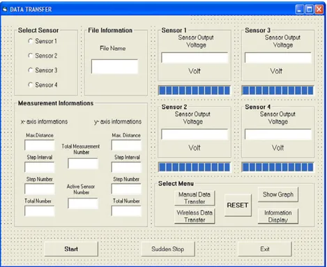
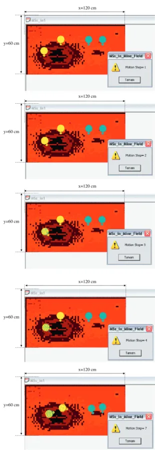
Autonomous navigation of robotic units in mobile sensor network
Tam metin
Şekil
Benzer Belgeler
Bir yayınevi sahibi beni arayarak Aziz Nesin’in öykülerinden olan bir kitabı çevirmemi istedi.. Kitap
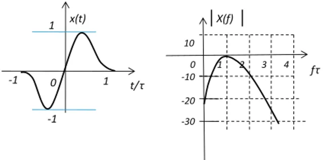
High-energy amplification to the ~1 µJ-level has been demonstrated by several groups at this wavelength range with low average powers using with LMA fiber amplifier
Şekil 33: Atasal HepG2 hücreleri, monoklonal anti-LPP2 antikoru ile karşılaşan atasal HepG2 hücreleri, pSilV1 plazmidi ile transfekte edilmiş ve VANGL1 geni sessizleştirilmiş 2
Araştırmada verilerin yapılan Pearson Korelasyon Analizi sonucunda cinsiyet, yaş, medeni durum, günlük çalışma süresi, haftada bakılan dosya sayısı ile
Bu kistlerin delinmesi ve daha sonra spontan olarak kapanması şeklinde devam eden siklusa bağlı olarak subdiafragmatik serbest hava oluşumu eğer klinik bulgularda uyumlu ise
9 Özkorkut, Nevin Ünal, “Basın Özgürlüğü ve Osmanlı Devleti’ndeki Görünümü”.. bilmek için gerekli olan ideolojinin yaratılması yer almaktadır. Bir çeşit
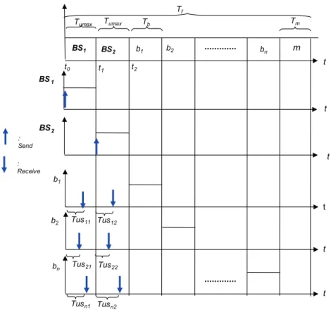
assume that this sensing range is limited and the total number of robots in the group can be large, a robot may not sense all other robots in the group.. one for
