Analysis of design parameters in safety-critical computers

JOURNAL OF LA_{TEX CLASS FILES, VOL. 14, NO. 8, AUGUST 2015 1}

Analysis of Design Parameters in Safety-Critical

Computers *

Hamzeh Ahangari, Funda Atik, Yusuf Ibrahim Ozkok, Asil Yildirim, Serdar Oguz Ata,

and Ozcan Ozturk, Member, IEEE

Abstract—Nowadays, safety-critical computers are extensively used in many civil domains like transportation including railways, avionics, and automotive. In evaluating these safety critical systems, previous studies considered different metrics, but some of safety design parameters like failure diagnostic coverage (C) or common cause failure (CCF) ratio have not been seriously taken into account. Moreover, in some cases safety has not been compared with standard safety integrity levels (IEC-61508: SIL1-SIL4) or even have not met them. Most often, it is not very clear that which part of the system is the Achilles heel and how design can be improved to reach standard safety levels. Motivated by such design ambiguities, we aim to study the effect of various design parameters on safety in some prevalent safety configurations, namely, 1oo2 and 2oo3, where 1oo1 is also used as a reference. By employing Markov modeling, we analyzed the sensitivity of safety to important parameters including: failure rate of processing element, failure diagnostic coverage, CCF ratio, test and repair rates. This study aims to provide a deeper understanding on the influence of variation in design parameters over safety. Consequently, to meet appropriate safety integrity level, instead of improving some parts of a system blindly, it will be possible to make an informed decision on more relevant parameters.

Index Terms—Safety, safety-critical computer system, IEC 61508 standard, common cause failure, Markov modeling.

F

1

I

NTRODUCTION

N

OWADAYS, safety-critical computers are obligatory constituents of many electronic systems that effect human life safety. Several areas of transportation industry like railways, avionics, and automotive, increasingly use such systems. To design a computer for safety-critical ap-plications, industrial safety levels such as European safety standard IEC 61508 (shown in Table 1) have been set. In this domain, safe microcontrollers with limited processing capabilities are available in the market for mostly control purposes. However, as systems become more and more complex and versatile, having safe processors with intensive processing capabilities becomes an essential need. Accord-ing to IEC 61508-2 standard, a sAccord-ingle processor can achieve at most SIL3 level. In most cases, safety critical applications in civil domains require a higher level of safety, such as SIL4. Hence, to answer this eminent need, a computing platform needs to be architected in system level with safety in mind.

In order to achieve such high standards, it is necessary to make improvements in numerous aspects of a general purpose system. Reliability of electronic components is the most obvious factor that needs to be satisfied for building a robust system. Besides, clever system design by means of available electronic components is as important as the quality of components themselves. Even with reliable and

• H. Ahangari, F. Atik, and O. Ozturk are with the Department of Computer Engineering, Bilkent University, Ankara, Turkey.

E-mail:{hamzeh, funda.atik, ozturk}@cs.bilkent.edu.tr.

• Y. I. Ozkok, A. Yildirim, and S. O. Ata are with Aselsan Corporation, Ankara, Turkey.

E-mail:{yozkok, asily, oguzata}@aselsan.com.tr.

* This study is an extension of our previous work [2] providing additional safety design parameters, illustration of reliability, availability, and initial unsafe state of systems with respect to SIL1-SIL4 levels in 2D plane, and a new approach for simplifying Markov chain.

TABLE 1: Safety levels in IEC 61508 standard for high demand/continuous systems (PFH: average frequency of a dangerous failure of safety function per hour, SIL: Safety Integrity Level) [16].

10−9 ₆ PFH of SIL4 < 10−8 10−8 6 PFH of SIL3 < 10−7 10−7 6 PFH of SIL2 < 10−6 10−6 ₆ PFH of SIL1 < 10−5

robust parts, safety goals may not be achieved without safety aware design process. Prevalent design issues like perfect printed circuit board, EMC/EMI isolation, power circuitry, fail rates of equipment etc., are examples of com-mon quality considerations. However, in critical systems, in addition to these, some other less obvious issues have to be observed.

The ratio of Common Cause Failures (CCFs), meaning the ratio of concurrent failure rate (failures among redun-dant channels) over total failure rate, has great impact on system safety. The percentage of failures the system is able to detect by means of fault detection techniques also has a direct effect on safety. This is because undetected failures are potential dangers. To avoid such undetected failures, an important factor is the frequency and the quality of system maintenance. Frequency and comprehension of the system tests (automatically or by technicians) to repair or replace the impaired components, can guarantee the required safety level by removing transient failures or refreshing worn-out parts.

As safety is a very wide subject, the main objective of this paper is to investigate the sensitivity of system safety to

some crucial design parameters. Three widespread configu-rations; 1oo1, 1oo2, and 2oo3; with known values of param-eters, are assumed as base systems. For these systems, we evaluated individual parameters that contribute to safety. In this paper we target high demand/continuous systems, where the frequency of demand to run the safety function is more than one per year, unlike low demand systems where it is less than one per year [16]. Average frequency of a dangerous failure of safety function per hour (PFH), is the safety measure for high demand/continuous systems, while probability of failure on demand (PFD), is the measure for low demand systems. PFH is defined as rate of entering into unsafe state, while PFD is defined as probability of being in unsafe state.

This paper is organized as follows: In Section 2, some of the recent works are reviewed and our motivation is given in more detail. In Section 3, definition and modeling for considered design parameters are described. In Section 4, base systems and their Markov modeling are proposed. In Section 5, experimental results are discussed, while Section 6 discusses a simplified Markov modeling in safety calcula-tions. Finally conclusion is given in Section 7.

2

R

ELATED

W

ORKS AND

M

OTIVATION

During the design process, concentrating on multiple as-pects of design altogether for the purpose of improvement can be complicated. Normally, if the prototype design does not meet the requirements, it is rational to find the system’s bottleneck and focus on it. In safety-related designs, by knowing the share that each parameter provides to safety, the designer can decide where to put more emphasis to improve the outcome with least amount of effort. Here, we discuss some of the safety-critical computer system designs in literature, which considered a subset of safety design parameters due to complexity.

In [15], authors designed a redundant computer system for critical aircraft control applications, and an acceptable level of fault tolerance is claimed to be achieved with using five redundant processors and extensive error detec-tion software. In [6], two dual-duplex and Triple Modular Redundancy (TMR) synchronous computer systems have been built using military electronic parts. While authors try to improve the system safety, the effect of CCFs are not

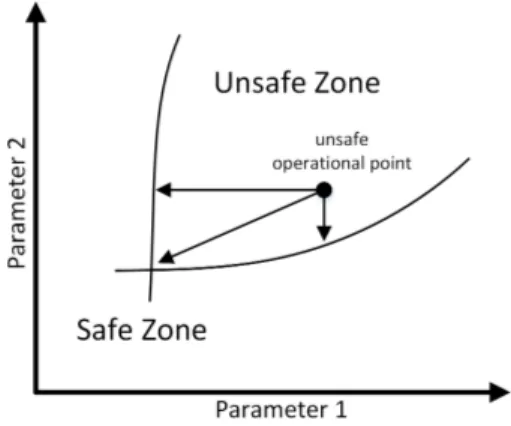
Fig. 1:Safety goal should be achieved by the most eco-nomical improvement.

assessed in addition to the diagnostic coverage for the TMR system. Besides, the achieved safety level is not compared to any standard level. In microcontroller-based SIL4 software voter [9], SIL4 level is claimed to be obtained. Nevertheless, neither failure coverage, nor CCFs are assessed in sufficient details. Similarly, in [5], authors target safe computer system for a train, which is not compared to standard levels, and does not consider CCFs or diagnostic coverage.

These approaches, either lack of considering some of the most influential safety design parameters or methodology to assess the system safety level with respect to standards. Thus, these studies are incomplete to be considered for real safety-critical applications due to complexity of taking all parameters into account. This stimulated us to have an anal-ysis on a few safety architectures also used in above studies. By showing the sensitivity of safety to each such parameter, we aim to provide a comparative understanding of these occasionally ignored parameters. This can help practitioners to select most appropriate parameter for improving the safety. Depending on the constraints, the most appropriate parameter can be translated to the one that leads to cheapest, fastest, or easiest system modification (as shown in Figure 1).

In [12], authors model a safety-related system in low de-mand mode using Markov chain to calculate PFD measure, in a way that is explained in the respective standard [18]. Several parameters such as CCF, imperfect proof testing, etc. are integrated into the model to investigate their influence over safety. However, in our work, we focus on PFH, where its calculation is not as straightforward as PFD. Moreover, we include additional parameters such as frequency of online testing, self-testing, etc., with sensitivity analysis for each parameter.

There have been many efforts related to generalized formula for PFH for M-out-of-N (MooN) architectures. The work proposed in [4] develops a set of generalized and simplified analytical expressions for MooN architectures by considering partial proof tests, while slightly taking the CCF contributions into account. In [11], probabilistic analysis of safety for MooN architectures is proposed when considering different degrees of uncertainty in some safety parameters such as failure rate, CCFs, and diagnostic coverage, by com-bining Monte Carlo sampling and fuzzy sets. Emphasizing the significance of CCF impact over safety in redundant systems, in [3], authors explore the criticality of beta-factor on safety calculations. Specifically, they address PFD mea-sure for a typical 1oo2 system. Influence of diversity in re-dundancy (i.e. implementing rere-dundancy with components technologically diverse) over CCF is assessed in [14] by a design optimization approach for low demand systems.

3

S

AFETY

P

ARAMETERS

I

N

O

UR

A

NALYSIS

In this section, we review the definition and modeling of design parameters that effect safety. It is assumed that the safety-critical computer system is composed of multiple redundant processing elements since such replication is recommended by safety standards.

3.1 Processing Element Failure Rate

A safety-critical computer system is composed of one or more redundant processing elements (PEs, and also

gen-JOURNAL OF LA_{TEX CLASS FILES, VOL. 14, NO. 8, AUGUST 2015 3}

Fig. 2: βmodels for duplicated and triplicated systems [8]. Here, β2= 0.3 of β, while β is split into 0.3β + 0.7β.

erally called channels), connected to each other by commu-nication links. Generally, there is no extraordinary require-ment regarding reliability of PEs. Due to low quantity and high cost of these systems, components are not necessarily designed for reliability purposes. Most often, a PE is a regu-lar processing module, built from available Commercial-Off-The-Shelf (COTS) electronic parts including microprocessor, memory, power circuitry, etc. In this study, we take a PE as a black box, assuming it comes with a single overall failure rate λP E, or simply λ.

3.2 Common Cause Failure (CCF)

According to IEC 61508-4 standard [16], Common Cause Failure (CCF, or dependent failure) is defined as concurrent occurrence of failures in multiple channels (PEs) caused by one or more events, leading to system failure. The β factor represents the fraction of dangerous failures that is due to CCF. Typically, for a duplicated safety system, β value is around a few percent, normally less than 10%. In safety standards, two β values are defined for detected and undetected failures (βDand β), while here we only assume a single β value for both. Assuming that CCF ratio between two PEs is taken as β, by using the extended modeling and notations shown in [8], we make the following observations for all systems in this work:

• 1oo1 configuration: Since there is no redundant PE, β1oo1= 0.

• 1oo2 configuration: As depicted in Figure 2, the β of system is only related to CCFs between two PEs. Therefore, β1oo2= β.

• 2oo3 configuration: As depicted in Figure 2, the overall β of 2oo3 system is related to mutual CCFs, plus CCFs shared among all three PEs. Note that by definition, the CCF ratio between every two PEs is taken as β. The β2 is defined as a number in [0, 1] range, expressing part of β which is shared among all three PEs [8]. For a typical 2oo3 system, we assume β2= 0.3 of β, making β2oo3= 2.4β (see Figure 2). The two parameters, β and β2, indicators of mutual and trilateral PEs isolation, are evaluated in our analysis.

3.3 Failure Diagnostic Coverage

According to IEC 61508-4 [16], Diagnostic Coverage (C or DC) is defined as the fraction of dangerous failures detected

by automatic online testing. Generally two complementary techniques are employed to detect failures, self-testing and comparison. Self-testing routines run upon each PE to di-agnose occasional failures autonomously and they usually detect absolute majority of failures, normally around 90%. Second diagnostic technique is data comparison among re-dundant PEs for detecting the rest of the undetected failures. Hence, generally we can express C as:

C = Cself test+ Ccompare≈ 1

As formulated in [7], we use the following expressions to describe the system’s C rate. According to the referred formulation, the total C is expressed as:

C = Cself test+ (1 − Cself test) · k

More specifically, k is the efficiency of comparison test. Since the comparison method is more effective against indepen-dent failures (none-CCFs), it is reasonable to differentiate between C rate of CCF and independent failures. Therefore, two variants of former expression can be derived:

Ci= Cself test+ (1 − Cself test) · ki Cc= Cself test+ (1 − Cself test) · kc Here ki_{and k}c_{are two constants, 0 6 k}i_{, k}c

6 1, describing the efficiency of comparison for either of two classes of failures. Since comparison is less effective against CCFs, the kc _{value is low, generally less than 0.4, while k}i _can be close to one [7]. Therefore, normally Cc

6 Ci. Three representative parameters; Cself test, kc and ki; are used in our analysis.

3.4 Test and Repair

Based on the IEC 61508 standard, two forms of test and repair have to be accessible for safety systems: online test and proof test. In online test (or automatic test), diagnostic routines run on each channel periodically, while system is available. As soon as a failure is detected, the faulty channel (or in some configurations the whole system) is supervised to go into fail-safe mode to avoid dangerous output. There-after, system tries to resolve the failure with immediate call for personnel intervention or a self commanded restart without human intervention. For transient failures, a system restart can be a fast solution, while for persistent failures switching to a spare PE or system, provides a faster recovery. In any case, online repairing is supposed to last from a few minutes to a few days. Repair rate is denoted by

µ

OT which

is defined as 1/M RTOT (M RT : mean repair time). The tD parameter is the time to detect a failure in online testing. There is no direct reference to this parameter in the standard, probably because it is assumed to be negligible with respect to repair time. However, it has been considered in literature [10]. M T T ROT(mean time to restoration) is mean total time to detect and repair a failure (see Figure 3). Some systems support partial recovery which means repairing a faulty channel while rest of the system is operational (like in 2oo3 configuration). Restarting only the faulty PE (triggered by operational PEs), can make it operational again. However, if the fault is persistent, such recovery is not guaranteed. Three parameters tD,

µ

OT and availability of partial recovery are

Fig. 3: Illustration of test-repair abbreviations in safety standards [16], [18]. Top: online test, bottom: proof test.

Proof test (or offline test or functional test) is the second and less frequent form of testing, whereby the periodic system maintenance process is performed by technicians. During such a maintenance, system is turned off and deeply examined to discover any undetected failure (not detected by online diagnostics) followed by a repair or replacement of defective parts. Test Interval (T I) defines the time interval at which this thorough system checking is performed and is typically from a few weeks to a few years. In such a scenario, repair time is negligible relatively. M T T RP T is the mean time to restoration (detect and repair as shown in Figure 3) from an undetected failure, and on average is taken as T I/2 [18]. Test and repair rate is denoted by

µ

P T = 1/M T T RP T. The

µ

P T is another parameter considered in our analysis.

4

B

ASE

S

YSTEMS

In this section, we define two prevalent safety configura-tions, 1oo2 and 2oo3 plus simple 1oo1 as a reference, for our analyses. Configurations are modeled by Markov modeling by employing all the aforementioned safety design param-eters. The assigned set of default values for parameters specify the initial safety point for each system.

4.1 Assumptions

In this study, we make the following assumptions: Typically, safe processor is responsible for running user computations. At the same time, it is in charge of checking the results for possible failures and taking necessary measures (in other words, running safety functions). The Markov models

Fig. 4: High level view of triplicated and duplicated systems.

presented in this paper are counted for safety functions. All channels (PEs) are asynchronous and identical (homo-geneous) and connected to each other by in-system links, whereby software voting and comparison mechanisms op-erate (Figure 4). In this work, our focus is on processing elements (PEs), while I/O ports and communication links are assumed to be black-channel, by which safety is not affected. This assumption can be realized by obeying stan-dards applied for safe communication over unsafe mediums (e.g. EN-50159). Our focus is on high demand/continuous safety systems, where the frequency of demand to run safety function is greater than one per year. Specifically, the safety function of the system detects and prevents any erroneous calculation result on PEs. These systems are assumed to be single-board computers (SBCs), meaning all redundant PEs reside on one board. It is assumed that partial recovery (as defined in Section 3.4) makes a faulty PE operational again. In the case of persistent failures, this can be realized by switching into spare PEs. Another simplifying assumption is that a CCF failure is detectable by all PEs or by none of them.

4.2 Default Parameters

For safety parameters which we intend to investigate in this study, we assign a set of default values to define an initial safety point for each system (shown in Table 2). In our experiments, we will sweep each parameter around the default value and illustrate how safety is affected. This way, the sensitivity of system safety with respect to that parameter will be revealed.

TABLE 2:Default values for safety design parameters.

Parameter Meaning Default value

λP E PE failure rate 1.0E-5/hour

Cself test Diagnostic coverage of self-testing [7] 0.90

ki _{Comparison efficiency for 0.90}

independent failures [7]

kc _{Comparison efficiency for CCFs [7] 0.40}

β CCF ratio between each two PEs 0.02

β2 Part ofβshared among three PEs [8] 0.3

tD Time to detect failure by online test 0 (negligible)

(inverse of online test rate)

µOT Online repair rate 1/hour

µP T Proof test and repair rate 0.0001/hour

(≈1/year) 4.3 Markov Models

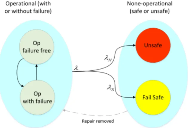
In this section, we give our safety configurations modeled by Markov chains. RAMS (Reliability, Availability, Main-tainability and Safety) measures are calculated according to guidelines suggested in ISA-TR84.00.02 [18] and IEC 61165 [17] standards, along with previous studies [1]. States are divided into two main categories; ’up’ (or operational) and ’down’ (or none-operational). In up states, the system is able to correctly run safety functions. Up state is either all-OK initial state or any state with some tolerable failures. Down states are those in which system is not able to correctly run safety functions, either intentionally as in the fail-safe state or unintentionally as in unsafe (hazardous) state. System

JOURNAL OF LA_{TEX CLASS FILES, VOL. 14, NO. 8, AUGUST 2015 5}

Fig. 5:Unsafe (hazardous) and safe failure rate.

moves into fail-safe/unsafe state if there are intolerable number of dangerous detected/undetected failures present. As soon as a dangerous failure is detected, system may either tolerate it (like the first detected failure in 2oo3 system) or enter into fail-safe state. On the other hand, if the failure is left undetected, system may inadvertently tolerate it (like first undetected failure in 1oo2 or 2oo3 systems) or enter into unsafe (hazardous) state.

PFH is defined as the rate of entering into an unsafe state. For safety calculation purposes, repair transitions from down states toward up states are removed, as in the case of reliability calculation [17]. Note that the repairs inside up states should not be removed. All of the following Markov models are in full form before repair removal. From the total failure rate, λ, only the hazardous part, λH, should be considered (as shown in Figure 5). The details of required formulation for decomposing λ into λHand λSis explained in the literature [13]. Authors used an approximation ( [13], Eq. 6) to conclude the following formula (PH: Probability of being in hazardous state, PS: Probability of being in fail-safe state, PHS = PH+ PS, PHS0 : derivative of PHSwith respect to time): λH = P_HS0 1 − PHS · PH PHS

Generally, probabilities of the system over time is de-scribed with the following set of differential equations:

P_1×n0 = P1×n· An×n,

where P is vector of state probabilities over time, P0 is derivative of P with respect to time, n is number of states, and A is transition rate matrix. Abbreviations used in Markov chains are listed in Table 3.

TABLE 3:Other abbreviations and symbols.

D Dangerous failure, a failure which has potential to put system at risk (only such failures are considered in this paper).

C Diagnostic coverage factor is the fraction of failures detected by online testing.

DD Dangerous detected failure, a dangerous failure detected by online testing.

DU Dangerous undetected failure, a dangerous failure not found by online testing.

CCF Common cause failure (dependent failure). λ Total failure rate of component or system. λi _{Independent failure rate of component or system.}

λc CCF failure rate of component or system. λDD DD failure rate of component or system.

λDU DU failure rate of component or system.

s, d, t Number of redundancies (single, dual or triple).

1oo1 Configuration: The single system is composed of a single PE without any redundancy. Hence, all failures are independent (none-CCF) and can only be detected by self-testing. If failure is detected, next state is fail-safe, otherwise it is unsafe (Figure 6). Transition terms for 1oo1 system are (ki_{= 0, C}i_{= C}

self test):

λDDs = Ci· λP E λDUs = (1 − Ci) · λP E λDs = λDDs + λDUs = λP E

Transition rate matrix for illustrated Markov will be as follows: A =    −λDs λDUs λDDs µP T −µP T 0 µOT 0 −µOT   

1oo2 Configuration: According to IEC 61508-6, 1oo2 sys-tem consists of two parallel channels which can both run the safety functions. However, only one dangerous-failure free channel is sufficient to keep the system safe. In this configuration, a single DU is tolerable which means that hardware fault tolerance (HFT) is equal to one. No DD failure is tolerated and system immediately enters into fail-safe mode (Figure 7). Generally, 1oo2 system has high fail-safety

Fig. 7:Markov model for 1oo2 system.

against DU failures and low availability against safe failures. It is assumed that online repair does not remove undetected failures in such cases. Note that in Figure 7, since the failure in state (2) is undetected or hidden, the system seemingly works with two operational channels. Therefore, the system has similar behavior against DD failures in both state (1) and state (2). However, in fact the faulty channel is not counted as operational. Because state (2) is one step closer to unsafe state than state (1). Transition terms used for 1oo2 system are: λi_DUd = 2[(1 − Ci) · (1 − β1oo2)]λP E λc_DUd = [(1 − Cc) · β1oo2]λP E λDDd = λiDDd + λ c DDd = (2 · Ci· (1 − β1oo2) + Cc· β1oo2)λP E λDd = λDDd + λDUd = λi_DDd + λc_DDd + λi_DUd + λc_DUd

Transition rate matrix for illustrated Markov will be as follows: A =          −λDd λiDUd λDDd 0 λcDUd µP T −(λDDd+ 0 λDDd λDUs λDUs + µP T) µOT 0 −µOT 0 0 0 µOT 0 −µOT 0 µP T 0 0 0 −µP T         

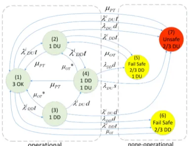
2oo3 Configuration: Similar to 1oo2, 2oo3 is also capable of tolerating one DU failure, meaning hardware fault tolerance (HFT) is equal to one. Besides, it has higher reliability (continuity of operation) due to being able to tolerate a single DD failure, similar to 2oo2 system (note that 2oo2 is not discussed here). Therefore, in literature, 2oo3 is known to have benefits of both 1oo2 and 2oo2 at the same time (as shown in Figure 8). However, due to more number of vulnerable channels (since the total failure rate of all channels increases with higher number of channels), 2oo3 is neither as safe as 1oo2, nor as reliable as 2oo2. Note that, in such a system, we assume online repairing does not remove undetected failures. In this figure, the µ∗OT edges represent partial recovery (explained in Section 3.4). Transition terms for 2oo3 system are (β2= 0.3):

Fig. 8:Markov model for 2oo3 system.

λi_DUt = 3 · [(1 − Ci) · (1 − 1.7β)]λP E λcDUt = [(1 − C c ) · 2.4β]λP E λDDt = λiDDt + λ c DDt = [3Ci· (1 − 1.7β) + Cc_{· 2.4β]λ} P E λDt = λDDt + λDUt = λiDDt + λ c DDt + λ i DUt + λ c DUt

Transition rate matrix for illustrated Markov will be as follows: A =                −λDt λiDUt λiDDt 0 0 λcDDt λcDUt µP T −µP T−λDDt 0 λiDDt λ c DDt 0 λDUd −λDUd µ∗_OT 0 −λDd λDUi d 0 λDDd λcDUd −µ∗ OT µP T µ∗OT 0 −µP T−λDDd λDDd 0 λDUs −µ∗ OT−λDUs 0 µOT 0 0 −µOT 0 0 µOT 0 0 0 0 −µOT 0 µP T 0 0 0 0 0 −µP T               

5

E

XPERIMENTAL

R

ESULTS AND

D

ISCUSSION

In this section, we investigate the influence of aforemen-tioned parameters over PFH measure through solving Markov models of four configurations: 1oo1, 1oo2, and 2oo3 without/with partial recovery (2oo3 and 2oo3-PR). First, we give the initial state of these configurations with the default values for RAMS measures - reliability, availability, and safety (PFH, not PFD).

5.1 Reliability and Availability

Reliability function, which is defined as probability of con-tinuously staying operational, is depicted in Figure 9. De-spite high safety level, the 1oo2 suffers from high rate of false-trips (transitions into fail-safe state), even more than the simple 1oo1. This follows from the fact that total failure rate of 1oo2 is around 2λ, and any single DD failure brings

JOURNAL OF LA_{TEX CLASS FILES, VOL. 14, NO. 8, AUGUST 2015 7}

Fig. 9:Reliability functions for base systems (refer to Table 2 for fixed parameter values).

Fig. 10:Steady state operational availability value for base systems with β variation (1oo1 is not shown, refer

to Table 2 for fixed parameter values).

whole system into fail-safe state. This is the cost paid for having high safety with a simple architecture. Moreover, note that if partial recovery is not provided, more complex 2oo3 system is not much better than 1oo2. Because, total failure rate is around 3λ, and two consecutive DD failures lead to fail-safe state. With partial recovery, the faulty PE with DD failure is quickly recovered largely reducing the probability of having two consecutive DD failures. Supe-riority of systems for operational availability at time=∞ (steady state availability), at very low β value (which is not practically achievable), are as expected (see Figure 10). However, as CCF rate increases, their order is swapped. This is due to the fact that staying more in operational states means higher probability of being exposed to DU CCFs and having a direct jump into unsafe state which takes considerable time to be recovered from. Nevertheless, for a typical and achievable β = 0.02, availability values are almost same, except 1oo1 which is by far the lowest (1oo1 is not shown).

5.2 Safety Sensitivity Analysis

In this section, we show the effect of variation in each of aforementioned parameters around defined default value, over PFH value. Mathematically, the following experiments show the partial derivations, ∂P F H/∂p, where p is one of

Fig. 11:Effect of λP Evariation over safety (refer to Table 2 for fixed parameter values).

the safety parameters. SIL1-SIL4 safety levels are plotted by horizontal lines to show relative safety position. By such illustration of safety, designer perceives the distance of current design state from desired safety level. Besides, we also show a few pairs of relevant parameters in 2D-space. At initial states of configurations specified by default pa-rameters, 1oo1 marginally could not achieve SIL2, while the rest are in SIL3 region. As explained before, generally 1oo2 is a safer configuration, while 2oo3 has higher reliability.

Sensitivity to λP E:

Figure 11 shows how safety is affected by different λP E values. It is understandable from both equations presented previously, and from Figure 11 that PFH is a linear function of λP E, meaning P F H = K · λP E (slope m=1 in logy-logx plane describes a linear function in y-x plane). Linearity im-plies that by just knowing the line slope which is achievable by having a single (λP E, P F H) point, and without solving the complicated Markov model or other techniques every time, safety of system can be tuned. For example, an order of magnitude (10X) improvement in λP E, results in shifting up one safety level (e.g. from SIL3 to SIL4).

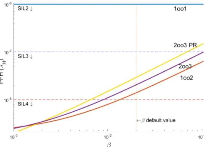
Fig. 12:Effect of β variation over safety (refer to Table 2 for fixed parameter values).

Fig. 13:Effect of β2 variation over safety (refer to Table 2 for fixed parameter values).

Sensitivity to β and β2:

β and β2are the indicators of mutual and trilateral isolation among PEs. It is a well-known fact that CCF failures have strong adverse effect on safety-critical systems. Figure 12 depicts how systems’ safety is affected by β variation. 1oo1 is independent from β as expected. One can observe from this figure that, for default parameters, it is quite difficult to get SIL4 through β improvement. Because by questionnaire method for β estimation (described in IEC 61508-6 [16]), β can hardly be estimated to be below 1%. A noticeable observation here is that similar to λP E, plots are almost linear in y-x plane (linear in logy-logx plane with slope of m=1), meaning P F H = K · β. Actually, this observation is only valid when β is not too small, that is for β > 0.5%. According to IEC 61508-6, the β below this range is not realistic. This linearity can be explained by dominance of linear CCF terms in formulations, which makes adjustment of safety by tuning β parameter easily, without needing to solve complicated mathematical models.

The β2is defined as a number in [0, 1] range, expressing part of β which is shared among all three PEs [8], where it is typically in 0.2-0.5 range. While 1oo2 is independent from it, increase in β2deteriorates PFH in triplicated systems by intensifying CCF effect (see Figure 13). One good design

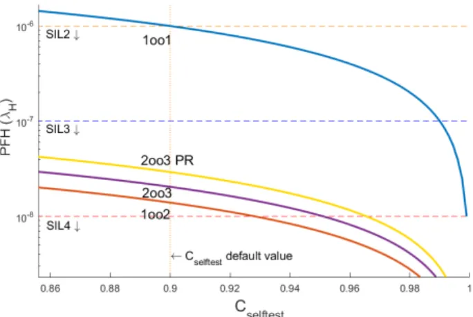
Fig. 14:Effect of Cself testvariation over safety (refer to Table 2 for fixed parameter values).

Fig. 15:Effect of ki_{variation over safety (refer to Table} 2 for fixed parameter values).

practice to prevent such issue is to avoid sharing common resources among all PEs. For example, communication links or power supply lines which are shared among all three PEs can be avoided.

Sensitivity to Cself test:

According to formulas in section 3.3, self-testing is assumed to be equally effective for both CCFs and none-CCFs. As shown in Figure 14, variation in this parameter does not have a significant effect in the superiority of systems, similar to variation in λP E. For achieving SIL4 in the 1oo2 system, the Cself test has to be increased 2-3%, while in 2oo3, it is more difficult, where at least 5% improvement is required (default of Cself test= 0.9).

Sensitivity to ki_: ki

is a constant which specifies the efficiency of comparison among PEs for detecting independent failures. Comparison is expected to be more efficient against none-CCFs than CCFs (ki= 0 for 1oo1). In Figure 15, there is an unexpected behavior as ki has almost no sensible (or very small) in-fluence on safety. The main reason for such observation is the absolute dominance of CCFs in above systems. More

Fig. 16:Effect of kcvariation over safety (refer to Table 2 for fixed parameter values).

JOURNAL OF LA_{TEX CLASS FILES, VOL. 14, NO. 8, AUGUST 2015 9}

Fig. 17:Simultaneous improvement of β-factor and kc to reach SIL4 level (refer to Table 2 for fixed parameter

values).

precisely, any DU CCF takes the whole system into unsafe state. However, two consecutive DU independent failures have to occur to cause the same situation which is far less probable. This is translated to an order of magnitude less influence of none-CCFs over safety. As a result, these systems seem to be rather insensitive to ki.

One possible incorrect conclusion from this observation is to give up comparison for independent failures. But the fallacy is that whether a failure is dependent or not is not distinguishable before detection. As we will see, kc_{still has} considerable effect on safety and as a result, comparison cannot be ignored. Since kc is usually as low as 0.1-0.4, a relaxed comparison mechanism that leads to ki_{value as low} as kc _{is completely acceptable. Because it is enough to just} have a reasonable value for kc.

Sensitivity to kc:

kcis a constant which specifies the efficiency of comparison among PEs for detecting CCFs. In both 1oo2 and 2oo3 configurations, CCFs mostly have negative influence when compared to independent failures. Because a single inde-pendent failure is tolerable in both cases. By the definition

Fig. 18:Simultaneous improvement of Cself testand kc to reach SIL4 level (refer to Table 2 for fixed parameter

values).

Fig. 19:Effect of online repair rate variation over safety (refer to Table 2 for fixed parameter values).

of CCF, comparison is not expected to be very efficient against CCFs (kc = 0 for 1oo1). Nevertheless, experiments (as shown in Figure 16) show that kcstill has a considerable effect over safety.

In case when one parameter is not sufficient to achieve the required safety level, simultaneous improvements on multiple parameters can be tried. Figures 17 and 18 show SIL regions in 2-D space while target safety is possible with values on SIL4 border lines.

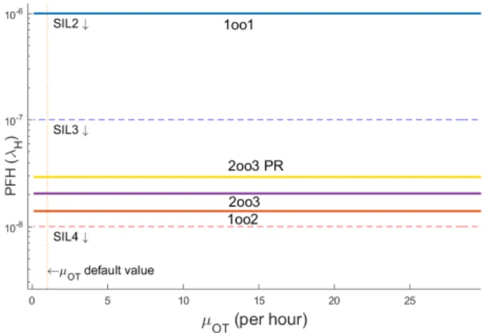
Sensitivity to µOT:

Online repair which is invoked after online failure detection, is either employed when a single PE is not operational due to a DD failure (provided that partial recovery is available) or when DD failures are tolerated until whole system is in fail-safe state (if partial recovery is not provided). Effect of repair rate in the former (only applicable to 2oo3 with partial recovery) is negligible. Since such repair does not reduce the number of DU failures. In the latter, effect is zero as expected (see Figure 19). Note that repairs from down states toward up states are removed in PFH calculation (see Figure 5). In practice, this parameter is useful for adjusting availability.

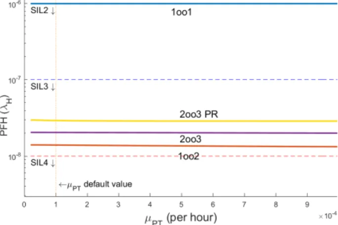
Sensitivity to µP T:

Proof test and repair occurs periodically in long periods of time (at T I or test interval) to remove DU failures. It is either employed when whole system is in unsafe state or while a DU failure is being tolerated (as in both safe configurations: 1oo2 and 2oo3). In the former, its effect on PFH is zero, similar to online testing, since repairs from down states are removed in PFH calculation. In the latter, although number of DU failures are reduced, due to dominance of CCF rate, such improvement is not observed in safety (see Figure 20). A single DU CCF failure can defeat safety in both 1oo2 and 2oo3, while two consecutive DU independent failures have to occur for leading to the same situation.

Sensitivity to partial recovery:

As illustrated earlier in Figure 9, if partial recovery (repair) is not provided, gain in reliability is not significant (which is the main advantage of 2oo3 over 1oo2). Therefore, usage of the more complex 2oo3 configuration is not logical. Unlike

Fig. 20:Effect of proof-test rate variation over safety (refer to Table 2 for fixed parameter values).

reliability, effect of partial recovery over safety (PFH) is reverse, which makes 2oo3 system slightly unsafer (shown in Figures 11 to 20) due to CCF dominance. When more PEs are operational, the probability of having a DU CCF failure is higher. This can be seen in Figure 12, where superiority of configurations are swapped at very low β values. Note that, this β value is not practically achievable.

Sensitivity to tD:

In online testing, time to detect a detectable failure (tD), is the time between occurrence and detection of a failure. Equivalently, δ = 1/tDis the frequency of online testing per hour. There is no direct reference to this parameter in IEC 61508 standard (except briefly for βDestimation), probably because in comparison to component failure rates, it is assumed to be negligible. In order to capture this parameter, an intermediate state is added to Markov chain for every

Fig. 21:An intermediate state is added to Markov chain, in which a DD failure has not been detected yet.

Fig. 22:Effect of δ (= 1/tD) variation over safety (refer to Table 2 for fixed parameter values).

DD failure transition (shown in Figure 21), in which the DD failure is temporarily considered as a DU failure. This additional state makes the Markov chain more complex. Therefore, due to Markov chain solution complexity, we only execute this for 1oo1 and 1oo2 configurations. Interme-diate states can be one of three types, operational, fail-safe or unsafe, as other normal states. But, for PFH calculation, they are not absorbing, meaning the transition of online testing is not removed. They also contribute to decrease the safety by causing more possibility of transition into unsafe states. Based on experimental results shown in Figure 22, we can observe that if δ < 0.1 per hour, safety level is slightly affected, while if δ < 0.01 per hour, the effect is significant.

6

A

PPROXIMATE

R

ATE

C

ALCULATION ON

M

ARKOV

C

HAIN

Our experimental results show the significance of β-factor in safety systems. Considering this fact and the Ω(n2₎ runtime required for Markov transition (matrix multiplica-tion formula given in Secmultiplica-tion 4.3, where n is the number of states), we propose a method for simplifying complex Markov chains into simpler ones. In this way, a quick and approximate failure rate can be calculated. Although CCF transitions have smaller rate value (multiplied by β), but due to jumping over several states, their impact on the system failure rate is decisive.

In the simple models depicted in Figure 23 (without on-line testing), two and three consecutive component failures move the system into fail state, while a single CCF has the same consequence (they are called as CCF2 and CCF3, depending on the number of jumps). In such a setting, it is desirable to compare the share of CCF and none-CCF transitions in the total failure rate. By using the conventional reliability formulations, failure rate is calculated for three scenarios: 1) full model, 2) keeping only CCF transition, 3) keeping only none-CCF transitions, including repairs. In the results shown in Table 4, failure rate is averaged over test interval (TI). As β increases, share of CCF transitions also increases. However, even at a smaller β value, order of the CCF rate is comparable to accurate result. While even solving such simple Markov chains requires computer applications, scenario 2 gives an immediate result in both models (system failure rate=CCF transition rate).

Fig. 23:Simple models for measuring CCF2 and CCF3 influences. λ = λP E, µ = µP T (refer to Table 2 for

JOURNAL OF LA_{TEX CLASS FILES, VOL. 14, NO. 8, AUGUST 2015 11}

TABLE 4:Failure rates of Figure 23 for three scenarios.

β = 0.02 β = 0.1 Full model (Figure 23:top) 8.7E-7 16.1E-7 Only CCF2 transition 2.0E-7 10.0E-7 None-CCF2 transitions 6.7E-7 6.7E-7 Full model (Figure 23:bottom) 1.08E-7 3.24E-7 Only CCF3 transition 0.6E-7 3.0E-7 None-CCF3 transitions 0.54E-7 0.54E-7

Following this observation, we propose a simplification technique for complex models. In this way, only the paths from start to fail state which include a CCF transition are preserved, while transitions or states not included in these paths are removed. The idea is explained on a simple Markov chain for a 1oo3 system shown in Figure 24. Using the same model as shown in Figure 2, transition terms are: λis = λP E λcd = β · λP E

λid = 2(1 − β) · λP E λc2t = 2.1β · λP E λit = 3(1 − 1.7β) · λP E λc3t = 0.3β · λP E

Fig. 24:A simple model for 1oo3 configuration.(refer to Table 2 for parameter values).

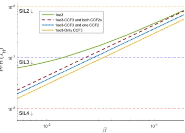
Starting from state (1), there are four different paths that lead to the fail state, namely, 1-4, 1-2-4, 1-3-4, and 1-2-3-4, where shorter paths have longer CCF jumps and more share in PFH value. To model this, we start with an empty Markov without any transition, and we add these paths one by one as shown in Figure 25. Solutions to these three approximate Markov chains and the main complete one are illustrated in Figure 26. As can be seen, even the simplest chain which includes only a single edge, provides a suitable approximation to estimate PFH and SIL level. In the simplest case, there is no need to solve the Markov as it is obvious that P F H = λc3t.

7

C

ONCLUSION

In this work, we analyzed the sensitivity of system safety to some critical design parameters in two basic multi-channel safe configurations, 1oo2 and 2oo3, where a 1oo1 system is used as baseline. All configurations have been modeled by Markov chains to examine at which safety integrity level (SIL) they stand, and how distant they are from the target. Hence, each safety parameter’s contribution on safety can be understood. Through these measurements, instead of

Fig. 25:Transition paths with longer CCF jumps are added one by one from top to bottom.

Fig. 26:Comparison between complete and simplified Markov chains of 1oo3 system (refer to Table 2 for fixed

parameter values).

blindly improving an unsafe system, designers can make an informed decision to select the most appropriate parameter for improvement. Through experiments, we showed that there is a linear relationship between safety (PFH) and two parameters: λP E and β, where the latter is due to CCF dominance. We also observed that parameters which have considerable effect on CCF rate are more appropriate candidates for safety level enhancement. These include λP E, β, Cself test, and kc. Additionally, we propose a method for

simplifying Markov chains in PFH calculation which can largely reduce the complexity to get an approximate result.

A

CKNOWLEDGMENTS

This research is supported in part by TUBITAK grant 115E835 and by TUBITAK Teydeb 1501 program grant 3140492.

R

EFERENCES

[1] D.J. Smith, ”Reliability, Maintainability and Risk: Practical Methods for Engineers”, Eighth Edition. Butterworth-Heinemann, Elsevier, pp. 436, 2011.

[2] H. Ahangari, Y. I. Ozkok, A. Yildirim, F. Say, F. Atik, O. Ozturk, ”Analysis of Design Parameters in SIL-4 Safety-Critical Computer”, Reliability and Maintainability Symposium (RAMS), 2017. [3] J. Borcsok, S. Schaefer, and E. Ugljesa, ”Estimation and evaluation

of common cause failures”, International Conference on Systems, ICONS, 2007.

[4] M. Chebila and F. Innal, ”Generalized analytical expressions for safety instrumented systems’ performance measures: PFDavg and PFH”, Journal of Loss Prevention in the Process Industries, pp.167-176, 2015.

[5] X. Chen, G. Zhou, Y. Yang and H. Huang, ”A newly developed safety-critical computer system for China metro”, IEEE Trans. Intell. Transp. Syst., vol. 14, no. 2, pp. 709-719, Jun. 2013.

[6] H. K. Kim, H. T. Lee and K. S. Lee, ”The design and analysis of AVTMR (all voting triple modular redundancy) and dual-duplex system”, Reliability Eng. Syst. Safety, vol. 88, no. 3, pp. 291-300, 2005.

[7] P. Hokstad, ”Probability of failure on demand (pfd)-the formulas of iec61508 with focus on the 1oo2d voting”, ESREL 2005, Gdansk, Polen, 2005.

[8] P. Hokstad and K. Corneliussen, ”Loss of safety assessment and the IEC 61508 standard”, Reliability Engineering and System Safety, vol. 83, pp. 111-120, 2004.

[9] M. Idirin, X. Aizpurua, A. Villaro, J. Legarda and J. Melendez, ”Implementation details and safety analysis of a microcontroller-based SIL-4 software voter”, IEEE Trans. Ind. Electron., vol. 58, no. 3, pp. 822-829, Mar. 2011.

[10] J. Ilavsky, K. Rastocny, and J Zdansky, ”Common-cause failures as major issue in safety of control systems”, Advances in Electrical and Electronic Engineering 11, no. 2, 2013.

[11] F. Innal, Y. Dutuit and M. Chebila, ”Monte Carlo analysis and fuzzy sets for uncertainty propagation in SIS performance as-sessment”, International Journal of Mathematical, Computational, Physical and Quantum Engineering, 2014.

[12] W. Mechri, C. Simon, and K. BenOthman, ”Switching Markov chains for a holistic modeling of SIS unavailability”, Reliability Engineering and System Safety, no. 133, 2015.

[13] K. Rastocny, and J. Ilavsky, ”Quantification of the safety level of a safety-critical control system”, 2010.

[14] A. C. Torres-Echeverria, S. Martorell, and H. A. Thompson, ”Design optimization of a safety-instrumented system based on RAMS+ C addressing IEC 61508 requirements and diverse redun-dancy”, Reliability Engineering and System Safety, no. 94, 2009. [15] J. H. Wensley, L. Lamport, J. Goldberg, M. W. Green, K. N. Levitt,

P. M. Melliar-Smith, R. E. Shostak, C. B. Weinstock, ”SIFT: Design and analysis of a fault-tolerant computer for aircraft control”, Proceedings of the IEEE, 1978.

[16] IEC-61508, Functional Safety of Electrical/Electronic /Pro-grammable Electronic Safety-related Systems, International Elec-trotechnical Commission (IEC), 2010.

[17] IEC-61165, Application of Markov techniques, International Elec-trotechnical Commission (IEC), 2006.

[18] ISA-TR84.00.02-2002, Safety Instrumented Functions (SIF) – Safety Integrity Level (SIL) Evaluation Techniques, Instrumentation Soci-ety of America (ISA), 2002.

Hamzeh Ahangari received BS degree in Computer Hardware from Sharif University of Technology, Iran and MS degree in Computer Ar-chitecture from University of Tehran, Iran. He is currently PhD student in computer engineering at Bilkent University, Turkey. His research interests are reliability, safety, reconfigurable architectures and high performance computing.

Funda Atik received the BS degree in Computer Engineering from Bilkent University. She is currently MS student at Bilkent University and her supervisor is Dr. Ozcan Ozturk. Her research interests include parallel computing, GPUs and accelerators, and computer architecture.

Yusuf Ibrahim Ozkok is employed as Lead Design Engineer at Aselsan Defense System Technologies Division. He has been involving design of mission critical and safety critical embedded systems for about 15 years. He has BS degree from Istanbul Technical University and MS degree from Middle East Technical University on Electrical and Electronics Engineering.

Asil Yildirim is a Senior Software Engineer at Aselsan Defense System Technologies Division. He is involved in development of safety critical embedded systems as embedded software engineer. He has BS and MS degrees in Electrical and Electronics Engineering from Middle East Technical University.

Serdar Oguz Ata is a Software Engineer at Aselsan Defense System Technologies Division. He is involved in development of safety critical embedded systems. He has BS degree in Electrical and Electronics Engineering from Middle East Technical University and MS degree in Computer Science from University of Freiburg. He is currently PhD student at Middle East Technical University.

Ozcan Ozturk has been on the faculty at Bilkent since 2008 where he currently is an Associate Professor in the Department of Computer Engi-neering. His research interests are in the areas of cloud computing, GPU computing, manycore accelerators, on-chip multiprocessing, computer architecture, heterogeneous architectures, and compiler optimizations. Prior to joining Bilkent, he worked at Intel, Marvell, and NEC.