1 23
Journal of Engineering Mathematics
ISSN 0022-0833
Volume 89
Number 1
J Eng Math (2014) 89:13-25
DOI 10.1007/s10665-014-9704-7
Analysis of heat transfer and entropy
generation for a low-Peclet-number
microtube flow using a second-order slip
model: an extended-Graetz problem
1 23
is for personal use only and shall not be
self-archived in electronic repositories. If you wish
to self-archive your article, please use the
accepted manuscript version for posting on
your own website. You may further deposit
the accepted manuscript version in any
repository, provided it is only made publicly
available 12 months after official publication
or later and provided acknowledgement is
given to the original source of publication
and a link is inserted to the published article
on Springer's website. The link must be
accompanied by the following text: "The final
publication is available at link.springer.com”.
J Eng Math (2014) 89:13–25 DOI 10.1007/s10665-014-9704-7
Analysis of heat transfer and entropy generation for a
low-Peclet-number microtube flow using a second-order
slip model: an extended-Graetz problem
Barbaros Çetin · Soheila Zeinali
Received: 17 April 2013 / Accepted: 11 April 2014 / Published online: 30 August 2014 © Springer Science+Business Media Dordrecht 2014
Abstract The classical Graetz problem, which is the problem of the hydrodynamically developed, thermally
developing laminar flow of an incompressible fluid inside a tube neglecting axial conduction and viscous dissipation, is one of the fundamental problems of internal-flow studies. This study is an extension of the Graetz problem to include the rarefaction effect, viscous dissipation term and axial conduction with a constant wall temperature thermal boundary condition. The energy equation is solved to determine the temperature field analytically using general eigenfunction expansion with a fully developed velocity profile. To analyze the low-Peclet-number nature of the flow, the flow domain is extended from−∞ to +∞. To model the rarefaction effect, a second-order slip model is implemented. The temperature distribution, local Nusselt number, and local entropy generation are determined in terms of confluent hypergeometric functions. This kind of theoretical study is important for a fundamental understanding of the convective heat transfer characteristics of flows at the microscale and for the optimum design of thermal systems, which includes convective heat transfer at the microscale, especially operating at low Reynolds numbers.
Keywords Extended-Graetz problem · Low Pe · Microtube · Second-order slip model 1 Introduction
Analysis of the hydrodynamically developed, thermally developing laminar flow of an incompressible fluid inside a tube neglecting axial conduction and viscous dissipation is known as the Graetz problem and is one of the fundamental problems of internal-flow studies. The Graetz problem was solved analytically by Graetz [1,2] and Nusselt [3] more than a century ago. Many studies extended the Graetz problem to include additional effects (such as axial conduction and viscous dissipation) and different channel geometries at the macroscale. An excellent review of the solution to the Graetz problem at the macroscale can be found elsewhere [4]. Recently, the Graetz problem
B. Çetin (
B
)· S. ZeinaliMechanical Engineering Department, Microfluidics & Lab-on-a-chip Research Group, ˙Ihsan Do˘gramacı Bilkent University, 06800 Ankara, Turkey
e-mail: [email protected]; [email protected] S. Zeinali
Table 1 Coefficients used in Eqs. (1) and (2) [21] a1 a2 b1 b2 1.0 0.5 2− FT FT 2γ γ+ 1 1 Pr 2− FT FT γ γ+ 1 1 Pr
has also been extended to study Hartmann flow [5,6], electrokinetic flow [7,8], and microscale flows by including the rarefaction effect [9–19].
With today’s facilities, the fabrication of channels with a size on the order of micrometers is not an issue (even the fabrication of microtubes with diameters of several micrometers/nanometers has become possible [20]). These kinds of small channels can easily constitute the elements of micro heat exchangers. For an effective and economical design of micro heat exchangers, the heat transfer characteristics of flow inside these microchannels need to be well understood. As the characteristic length (L) of the flow approaches the mean free path (λ) of the fluid, the continuum approach is no longer valid, and fluid flow modeling moves from a continuum to a molecular model. The ratio of the mean free path to the characteristic length of the flow is known as the Knudsen number (Kn= λ/L). For Kn varying between 0.01 and 0.1 (which corresponds to the flow of air in standard atmospheric conditions through a channel with a characteristic length of 0.7–7 µm), the regime is known as a slip-flow regime. In this regime, flow can be modeled by continuum modeling as long as the boundary conditions are modified to take into account rarefaction effects.
The general form of the boundary conditions for velocity and temperature can be written as follows:
u− uw= a1λ !∂u ∂n " wall+ a2 λ2 !∂2u ∂n2 " wall+ a3 λ2 !∂T ∂t " wall , (1) T − Tw = b1λ ! ∂T ∂n " wall+ b2 λ2 ! ∂2T ∂n2 " wall , (2)
where n and t are the normal and tangential directions, respectively. The first terms of Eqs. (1) and (2) are known as first-order boundary conditions, and the second terms are known as second-order boundary conditions [21]. The last term of Eq. (1) is known as thermal creep, which is the fluid flow in the direction from cold to hot if a tangential temperature gradient exists along the channel walls [22] (since the thermal boundary condition is constant wall temperature in this study, thermal creep term is set to zero). As the modeling moves to the edge of the slip flow regime (i.e., Kn approaches 0.1), the inclusion of the second-order terms improves the accuracy of the solution. There are many different second-order models with different coefficients [23]. In this study, the second-order model proposed by Beskok and Karniadakis [21], which is an accepted model for a slip-flow regime, is used. However, different second-order models can also be implemented in the current mathematical model by introducing the appropriate slip coefficients. The coefficients for the second-order model proposed by Beskok and Karniadakis [21] are given in Table1.
The characteristic lengths of the microchannels are very small; thus, viscous forces dominate inertial forces, leading to a low Reynolds number (i.e., Re ∼ 1.0) and a low Peclet number (Pe = Re Pr ∼ 1.0). For flows with a small Peclet number, the characteristic time of the convection and the diffusion becomes comparable, and the convection term no longer dominates the conduction term in the longitudinal direction. In this case, the axial conduction term cannot be neglected. The Graetz problem involving the inclusion of the axial conduction term has proven to be an interesting problem due to the existence of the non-self-adjoint eigenvalue problem. Accordingly, linearly independent eigenfunctions become nonorthogonal [24]. This interesting problem has been studied by many researchers for flows in macrochannels [25–35]. More recently, the effect of axial conduction is also discussed for Hartmann flow [5,6], for mixed electroosmotic and pressure-driven microflows [7,8], for slip flow in a slit channel [15,18], and for slip flow in a microtube [19].
This study extends the Graetz problem to include the rarefaction effect, viscous dissipation term, and axial conduction in a fluid in constant wall temperature boundary conditions. By defining the appropriate nondimensional
An extended-Graetz problem 15
Fig. 1 Geometry of
problem
parameters, the given problem is formulated in a similar form with its macroscale counterpart. The temperature distribution, Nusselt number, and local entropy generation are determined analytically using a general eigenfunction expansion and are obtained in terms of confluent hypergeometric functions. To fully explore the effect of axial conduction, the solution domain is extended from−∞ to +∞ and a step change in the wall temperature is implemented. A two-part solution of the temperature field is obtained, and the two solutions are matched at the entrance of the heated region. The present study is an extension of the previous study of Çetin et al. [19]. The extensions to the previous study can be stated as the (1) use of a constant wall temperature thermal boundary condition, (2) inclusion of a second-order slip model, (3) extension of the solution domain from−∞ to +∞, and (4) inclusion of the analysis of the entropy generation. The mathematical model is implemented using the
Mathematicasoftware package by which a wide range of results are possible to be obtained rapidly by using this analytical model with high precision compared to numerical solutions.
2 Mathematical model
Consider the laminar flow of an incompressible, viscous fluid flowing into a microtube at a constant temperature, Ti,
as shown in Fig.1. The flow is assumed to be steady-state, hyrodynamically developed flow. The microtube walls are maintained at temperature Tifor x ≤ 0 and Twfor x > 0. The thermophysical fluid properties are assumed to be
constant, and the free convection due to the temperature difference is neglected. The solution domain is separated into two regions: upstream (−∞ < x < 0) and downstream (0 < x < +∞) regions. The solutions are obtained for two regions, and the matching conditions are applied at the interface. By introducing the following dimensionless parameters [36], ¯r = rR, ¯x = x Pe R, θj = Tj− Tw Ti− Tw (j = 1, 2), ¯u = u um, Pe= Re Pr, Br = µu2m k(Ti− Tw) , (3) the governing energy equation, including the axial conduction, the viscous dissipation term, and the corresponding boundary conditions for the two regimes, can be written as
¯u 2 ∂θj ∂¯x = 1 ¯r ∂ ∂¯r # ¯r∂θj ∂¯r $ + 1 Pe2 ∂2θj ∂¯x2 + 32 Br (1+ 8 Kn − 8 Kn2)2¯r2 % for j= 1, −∞ < ¯x < 0, for j= 2, 0 < ¯x < +∞, (4) ∂θj ∂¯r = 0 ( j = 1, 2) at ¯r = 0 for − ∞ < ¯x < +∞, (5a) θj = (2 − j) − 2b1Kn ! ∂θj ∂¯r " + 4b2Kn2 ! ∂2θj ∂¯r2 " at¯r = 1 ( j = 1, 2), (5b) θ1→ 1 as ¯x → −∞, (5c) θ2→ θ2,∞ as ¯x → +∞, (5d)
where θj∞is the dimensionless fully developed temperature profile, and ¯u is the dimensionless fully developed
velocity profile for the slip-flow regime defined as [36] ¯u = 2(1− ¯r2+ 4 Kn − 4 Kn2)
The dimensionless numbers used in these equations are the Reynolds number (Re= umD/ν), Prandtl number
(Pr = ν/α), Knudsen number (Kn = λ/D), and Brinkman number (which indicates the relative importance of the heating of the fluid due to viscous dissipation for the heating of the wall). The matching conditions for the two solutions are the continuity of the temperature and the continuity of the heat flux at the entrance and can be written as
θ1= θ2 at ¯x = 0, ∂θ1
∂¯x = ∂θ2
∂¯x at¯x = 0. (7) The solution to the energy equation, Eq. (4), can be said to be the superposition of two solutions as
θj(¯r, ¯x) = φj(¯r, ¯x) + θj,∞(¯r) ( j = 1, 2), (8) where θj,∞ are the particular solutions for two regions, and the φj(¯r, ¯x) are the homogeneous solutions. The
governing equation and the boundary conditions can be separated. The governing equations and the corresponding boundary conditions for the particular solutions can be written as
∂ ∂¯r ! ¯r∂θ∂j,¯r∞ " = −(1 32 Br + 8 Kn − 8 Kn2)2¯r3 (j = 1, 2), (9) ∂θj,∞ ∂¯r = 0, (10a) θj,∞= (2 − j) − 2b1Kn ! ∂θj,∞ ∂¯r " + 4b2Kn2 ! ∂2θj,∞ ∂¯r2 " at¯r = 1, (10b) and the solutions can be obtained as
θj,∞= (2 − j) + & 2Br (1+ 8 Kn − 8 Kn2)2 ' ( 1− ¯r4+ 8b1Kn− 48b2Kn2 ) (j = 1, 2). (11) The homogeneous solutions, φj, can be further arranged by defining the following dimensionless parameters:
η= ¯rρs, ξ = ρs2(2− ρs2)x, *Pe= Pe ρs(2− ρs2)
, ρs2= 1
1+ 4 Kn − 4 Kn2, (12)
where ρsis the slip radius defined by Larrode et al. [11], which is a parameter that takes into account the rarefaction
effect. The introduction of these variables allows us to write the equation and the boundary conditions associated with φj(¯r, ¯x) as follows: (1− η2)∂φj ∂ξ = 1 η ∂ ∂η # η∂φj ∂η $ + *1 Pe2 ∂2φj ∂ξ2 (j = 1, 2), (13) ∂φj ∂η = 0 at η = 0 ( j = 1, 2), (14a) φj = −2b1Knρs !∂φ j ∂η " + 4b2Kn2ρs2 !∂2φ j ∂η2 " at η= ρs (j= 1, 2), (14b) and the matching conditions read as follows:
φ1= φ2 at ξ = 0, ∂φ1
∂ξ = ∂φ2
∂ξ at ξ= 0. (15)
Equation (13) has the same form as its macroscopic counterpart (i.e., macrotube flow without viscous dissipation). The differences are the viscous dissipation term and the temperature-jump boundary conditions, Eq. (14b) (although the temperature-jump boundary condition is different from that of the macrotube flow; from a mathematical point of view it is a homogeneous mixed-type boundary condition, which is an appropriate boundary condition to apply eigenfunction expansion). Setting Br= 0 and Kn = 0 would result in exactly the same problem for macrochannel
An extended-Graetz problem 17
flow. Macrochannel flow with low Pe was solved for both constant wall temperature [35] and constant wall heat flux [34] boundary conditions. Therefore, a solution procedure similar to that of [35] will be extended to take into account rarefaction and viscous dissipation effects.
The solutions of the temperature profiles in the upstream and the downstream regions can be represented by infinite series of eigenfunctions [5,6,34,35] as
φ1(η, ξ )= 1 + ∞ + m=1 AmFm(η)eλ2mξ, φ2(η, ξ )= ∞ + m=1 BmGm(η)e−βm2ξ. (16)
Introducing these solutions into Eq. (13) makes it possible to show that the functions Fm(η)and Gm(η)and the eigenvalues λm and βm satisfy the following eigenvalue problems:
d dη # ηdFm dη $ + λ2 m !λ2 m *Pe2 − 1 + η 2"ηF m(η)= 0, (17a) dFm dη =0 at η= 0, (17b) Fm(η)= −2b1Kn ρs! dFdηm " + 4b2Kn2ρs2 ! d2Fm dη2 " at η= ρs, (17c) d dη # ηdGm dη $ + βm2 ! βm2 *Pe2 − 1 + η2 " ηGm(η)= 0, (18a) dGm dη =0 at η= 0, (18b) Gm(η)= −2b1Kn ρs! dGdηm " + 4b2Kn2ρ2s! d 2G m dη2 " at η= ρs. (18c) The solutions to Eqs. (17) and (18) can be expressed in terms of confluent hypergeometric functions as
Fm(η)=1F1(a1; b1; z1)eλmη 2/2 , (19) Gm(η)=1F1(a2; b2; z2)e−βmη 2/2 . (20)
The arguments for the confluent hypergeometric functions are given as
a1=1 2 + λm 4 # λ2 m *Pe2 − 1 $ , b1= 1, z1= λmη2, (21a) a2=12 − β4m# β 2 m *Pe2+ 1 $ , b2= 1, z2= βmη2. (21b) Clearly, Eqs. (19) and (20) do not belong to the usual Sturm–Liouville system. However, it can be shown that the eigenfunctions Fm(η)and Gm(η)satisfy the following properties [35]:
ρs , 0 !λ2 n+ λ2m *Pe2 − 1 + η 2"F mFnηdη= % 0 if m= n, N (λm) if m̸= 0, (22a) ρs , 0 !β2 n+ βm2 *Pe2 + 1 − η2 " GmGnηdη= % 0 if m= n, N (βm) if m̸= 0, (22b) where N (λm)= ρs , 0 ! 2λ2 m *Pe2 − 1 + η2 " Fm2ηdη, (23a)
N (βm)= ρs , 0 ! 2β2 m *Pe2 + 1 − η2 " G2mηdη. (23b)
At this point, the eigenvalues λmand βmand the coefficients Amand Bmneed to be evaluated. The eigenvalues can
be evaluated using the wall boundary conditions. The coefficients can be determined using the matching conditions at ξ= 0 with the following equations:
1+ ∞ + m=1 AmFm(η)= ∞ + m=1 BmGm(η), (24a) ∞ + m=1 λ2mAmFm(η)= − ∞ + m=1 βm2BmGm(η). (24b)
Note that the eigenfunctions Fmand Gmare not mutually orthogonal (with reference to the standard Sturm–Liouville
problem) since the eigenvalues occur nonlinearly. By utilizing the boundary conditions and the expressions in Eqs. (22) and (23), the coefficients Am and Bm can be written as ratios of two integrals as follows (the details of
this derivation can be found elsewhere [35]):
Am= − , ρs 0 ! λ2m *Pe − (1 − η 2)"F mηdη , ρs 0 ! 2λ2 m *Pe − (1 − η 2)"F2 mηdη , (25a) Bm = , ρs 0 ! βm2 *Pe+ (1 − η 2)"G mηdη , ρs 0 ! 2β2 m *Pe + (1 − η 2)"G2 mηdη . (25b)
Knowing that the eigenvalues, eigenfunctions, and the coefficients Am, the temperature field, θ(¯r, ¯x), can be
determined. Knowing the temperature field, the local Nu can be determined from Nu¯x= −T D mean− Twall ! ∂T ∂r " r=R= − ! 2dθ d¯r " ¯r=1 θmean(¯x) at¯r = 1, (26) where θmeanis the dimensionless mean temperature defined as
θmean(¯x) = 2
1
,
0
¯uθ(¯r, ¯x)¯r d¯r. (27) Knowing the temperature field and the velocity field, the volumetric rate of entropy generation due to heat transfer and fluid friction losses can be written as [37]
SG = k T2 0 -!∂T ∂r "2 + ! ∂T ∂x "2. +Tµ 0 ! ∂u ∂r "2 , (28)
where the first term represents the entropy generation due to heat transfer, and the second term represents the entropy generation due to fluid friction (i.e., viscous dissipation). The volumetric rate of entropy generation can be put in dimensionless form, using the entropy generation number Ns(¯r, ¯x), as
Ns= SG SG,c = ! ∂θ ∂¯r "2 + 1 Pe2 ! ∂θ ∂¯x "2 +Br , ! d¯u d¯r "2 , (29)
An extended-Graetz problem 19
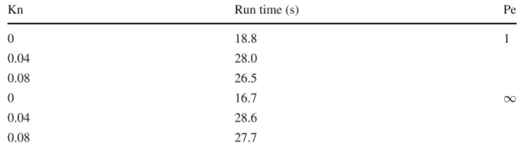
Table 2 Typical run-time
values for different Kn and Pe (Br = 0) Kn Run time (s) Pe 0 18.8 1 0.04 28.0 0.08 26.5 0 16.7 ∞ 0.04 28.6 0.08 27.7
where , is the dimensionless temperature difference, and SG,cis the characteristic entropy generation. , and SG,c
are defined as ,=Ti− Tw T0 , SG,c = k(Ti − Tw)2 R2T2 0 , (30)
where T0is the absolute reference temperature.
3 Results and discussion
The heat transfer characteristics of the extended Graetz problem is analyzed by solving the governing equation, Eq. (4), using superposition and a general eigenfunction expansion. Since the eigenvalues are not self-adjoint, the results are presented in terms of confluent hypergeometric functions. The procedure described in the previous section is coded using Mathematica. During the calculation, to improve the precision of the calculations, quadruple precision is achieved by use of the N function. The eigenvalues are obtained using the built-in FindRoot function, and the numerical integrations are performed using the built-in NIntegrate function. Kn is varied between 0 and 0.12, which are the applicability limits of the slip-flow regime. The coefficients b1and b2are taken respectively as
1.667 and 0.833 (FT = 1.0 [38], γ = 1.4, Pr = 0.7), which are the typical values for air, which is the working fluid
in many engineering applications.
The number of eigenvalues is observed to be important when the close vicinity of the entrance of the heating region is involved. It was observed that the convergence of the infinite series are slow in the vicinity of ξ = 0. This issue was also discussed in previous studies [35,39]. Following some test runs with different N , eigenvalues of N = 20 are used in the evaluation of the temperature distribution in this study. The results are plotted starting from different ξ values for the sake of the clarity of the figure. Concerning the 20 eigenvalues, the lower limit of 0.001 is chosen for ξ.
With the current mathematical model, the temperature profile within the channel can be obtained for a wide range of parameters. The results are presented in terms of the local Nu (which is the dimensionless heat transfer coefficient) and the average entropy generation number (which is the dimensionless entropy generation averaged over the cross-sectional area), which are the main parameters of interest to engineers in the design of thermal systems (e.g., optimal thermal design based on entropy generation minimization) [37].
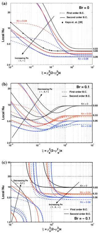
The computations were performed on a HP Z400 Workstation (Intel Xeon W3550, Quad core, 3.06 GHz, 16 GB RAM). It was observed with the present model that both the local Nu and the average entropy generation number can be evaluated rapidly. Some typical run-time values for the evaluation with 20 eigenvalues are given in Table2. A discussion of the effects of axial conduction, viscous dissipation, and rarefaction can be found elsewhere [10,11,15,17,19,36]. In this study, the main focus is the analysis of heat transfer, including the second-order model. Therefore, the figures are plotted to discuss the effect of the second-order model. Pe is varied between 1 and 5, and it is taken to be 106to demonstrate the Pe→ ∞ case. Figure2shows the local Nu variation for different
the inclusion of the second-order model affects Nu in different ways in the thermally developing and thermally developed regions. At the inlet, the temperature is almost uniform; therefore, the gradient of the temperature profile is very steep within the thermal boundary layer in the developing region. The inclusion of the temperature jump actually decreases heat conduction at the wall, which also reduces the local Nu. Since the temperature jump increases with Kn and the first-order model predicts a higher temperature jump than the second-order model, the local Nu decreases with increasing Kn and as the modeling moves from the first-order model to the second-order model. As the flow develops thermally, the gradient of the temperature profile within the thermal boundary layer decreases, and although the conclusion about the decreasing Nu for increasing Kn is still valid, the situation between the first-order and second-order models changes. Conduction heat transfer at the wall in the case with the second-order model decreases in the longitudinal direction, and eventually the Nu predicted by the first-order model somewhere in the developing region becomes higher than that of the second-order model. The Br number indicates the relative importance to the heating of the wall of the heating of the fluid due to viscous dissipation.
For gaseous flow in a microchannel, order-of-magnitude estimates for some parameters can be summarized as
O(µ)∼ 10−5Ns/m2, O(U
0)∼ 10−1− 10 m/s, O(k) ∼ 10−2− 10−1W/mK, and O(|Ti − Tw|) ∼ 10 K. With
these values, O(|Br|) ∼ 10−8− 10−2. A positive Br number means fluid is being cooled (i.e., the inlet temperature
is higher than the wall temperature). In this case, with Br = 0.1 (Fig.2b), Nu decreases in the developing region but then experiences an increase as the flow develops thermally. This increase is common in flow with viscous dissipation [17,36]. In previous studies, it was shown that the decrease in Br pushes the point where the increase begins further downstream. Because of this, Br is taken as|Br| = 0.1 since this case covers all the characteristics of the flow. At the region where the flow develops thermally, the heat generated within the fluid due to viscous dissipation becomes equal to the conduction heat transfer at the wall. Since with the inclusion of the slip flow at the wall, the gradient of the velocity profile decreases, which results in a reduction of viscous dissipation. This is why Nu decreases as Kn increases.
For a comparison of the results from the first- and second-order models, the combined effect of the slip flow and the temperature jump needs to be considered. The first-order model predicts a higher slip velocity at the wall, and hence lower viscous dissipation within the fluid, and lower conduction heat transfer at the wall. As a result, the first-order model predicts a higher bulk mean temperature and lower Nu than does the second-order model. Negative Br means fluid is being heated (i.e., the inlet temperature is lower than the wall temperature). In this case, with Br =−0.1 (Fig.2c), there exists a singular point where Nu goes to infinity. This is the point where the bulk mean temperature of the fluid becomes equal to the wall temperature. Beyond that location, fluid starts to heat the wall, which would be the undesired case in most practical applications that aim to heat the fluid. Again, the location of this singular point depends on Pe, but it does not depend on Kn or the slip model (the location of this singular point also moves further downstream with increasing Br). In the case where Br̸= 0, the effect of the slip models on Nu is more severe compared to the Br = 0 case. This is because for Br= 0, Nu changes mainly due to what is happening to the convection mechanism at the wall through the slip velocity and temperature jump. However, in the case where Br̸= 0, viscous dissipation is a result of the velocity field. On top of the convection mechanism at the wall, the thermal characteristics also change due to changes in the flow field. The second-order model predicts a velocity profile with a lower slip velocity compared to that of the first-order, which results in a steeper profile and, hence, higher viscous dissipation.
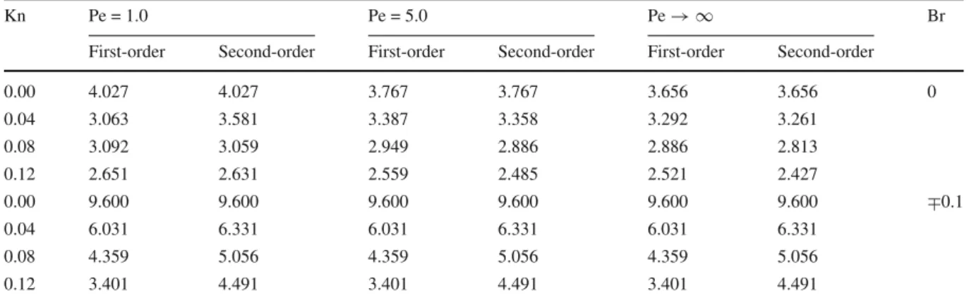
The present results are compared with the available results in the literature. A comparison of the results for Pe → ∞ (i.e., without axial conduction) and Br = 0 (i.e., no viscous dissipation) is presented in Table 3and plotted in Fig.2a for different Kn. As seen from the table and the graph, a good agreement is achieved with 20 eigenvalues. Fully developed Nu values (that is, the Nusselt number for a fully developed flow) for cases without viscous dissipation (Br = 0) and with viscous dissipation (Br ̸= 0) are given in Fig. 3and tabulated for differ-ent Br in Table4. For the case with Br ̸= 0, the fully developed Nu is not function of Br and Pe. Therefore, in Table4only single values are given for different Br and Pe. Nu∞decreases with increasing Kn and increases as it moves from the first-order to the order model. Moreover, the deviation between the first- and second-order models increases as Kn increases, which indicates the necessity of the second-second-order model as rarefaction increases.
An extended-Graetz problem 21
Fig. 2 Variation of local
Nu as a function of dimensionless axial coordinate for different Kn.
a Br = 0. b Br = 0.1. c Br = −0.1
(a)
(b)
(c)
Figure4illustrates the average entropy generation number for different Kn, Br, and Pe using the second-order model. For zero Br, the curves approach zero due to fact that the temperature of the fluid tends to be uniform and equal to the wall temperature, which diminishes entropy generation. For Br different than zero, since viscous dissipation is a source of heat generation, entropy generation does not diminish due to the finite temperature gradients within the microchannel. For high Pe, the temperature profile at the entrance of the heated section is close to being uniform;
Table 3 Comparison of Nu∞for present study with first-order model and available results from literature (Br = 0) Kn Pe= 1.0 Pe= 5.0 Pe→ ∞ Nu∞ [36] [4] Nu∞ [36] [35] Nu∞ [36] [17] 0.00 4.027 4.028 4.030 3.767 3.767 3.767 3.656 3.656 3.656 0.04 3.603 3.604 – 3.387 3.387 – 3.292 3.292 3.292 0.08 3.093 3.093 – 2.949 2.949 – 2.886 2.887 2.887
Fig. 3 Fully developed Nu
for different Kn. a Br= 0. b |Br| = 0.1
(b)
(a)
therefore, high temperature gradients exist in both the radial (close to the wall) and axial directions. As Pe decreases, these gradients decrease. With increasing Kn, the temperature jump at the wall decreases the gradient. Therefore, the entropy generation number decreases as Pe decreases and Kn increases.
4 Summary and future work
In this study, the extended Graetz problem, which includes the rarefaction effect, viscous dissipation term, and axial conduction within a fluid for constant wall temperature boundary conditions, is analyzed. A mathematical
An extended-Graetz problem 23
Table 4 Fully developed Nu values for different Kn, Pe, and Br
Kn Pe = 1.0 Pe = 5.0 Pe→ ∞ Br
First-order Second-order First-order Second-order First-order Second-order
0.00 4.027 4.027 3.767 3.767 3.656 3.656 0 0.04 3.063 3.581 3.387 3.358 3.292 3.261 0.08 3.092 3.059 2.949 2.886 2.886 2.813 0.12 2.651 2.631 2.559 2.485 2.521 2.427 0.00 9.600 9.600 9.600 9.600 9.600 9.600 ∓0.1 0.04 6.031 6.331 6.031 6.331 6.031 6.331 0.08 4.359 5.056 4.359 5.056 4.359 5.056 0.12 3.401 4.491 3.401 4.491 3.401 4.491
Fig. 4 Variation in average
entropy generation number as a function of
dimensionless axial coordinate for different Pe.
a Kn = 0. b Kn = 0.04
(a)
(b)
model is developed using a general eigenfunction expansion. The temperature distribution, local Nu, and local entropy generation are obtained in terms of confluent hypergeometric functions. To fully explore the effect of axial conduction, the solution domain is extended from−∞ to +∞, and a step change in the wall temperature is implemented. A two-part solution of the temperature field is obtained, and the two-parts of the solution are matched at the entrance of the heated region. The mathematical model is implemented using Mathematica. Using the current mathematical model, it is possible to obtain a wide range of results rapidly with high precision, as desired. These
parameters may be the key parameters in the design of thermal systems at the microscale. The effects of Kn, Br, and Pe on the local Nu, fully developed Nu, and local entropy generation are discussed. First- and second-order slip models are implemented to discuss the effect of rarefaction. It is found that for zero Br, the local Nu decreases with increasing Kn and decreases when the modeling moves from the first-order to the second-order model. In the case with viscous dissipation (Br̸= 0), the first-order model is found to predict a higher bulk mean temperature and lower Nu than the second-order model. It is also observed that the local entropy generation number decreases as Pe decreases and Kn increases.
The extension of the thermal boundary condition to constant wall heat flux seems to be straightforward. However, since this is a second-order model with a constant wall heat flux boundary condition, thermal creep enters the picture, which makes the velocity profile dependent on the tangential temperature gradient within the channel wall. Extension of the present study to include constant wall heat flux thermal boundary conditions will be one of our future research directions. Another important parameter (also associated with a constant wall heat flux thermal boundary condition) that is important at the microscale is the heat transfer that occurs within the channel wall since heat flow in a channel wall is comparable to heat flow within a microchannel due to the thick microchannel walls. Inclusion of axial conduction in channel walls will be another future research direction.
References
1. Graetz L (1883) Uben die wärmeleitungsfähigkeit von flüssigkeiten (On the thermal conductivity of liquids, part 1). Ann Phys Chem 18:79–94
2. Graetz L (1885) Uben die wärmeleitungsfähigkeit von flüssigkeiten (On the thermal conductivity of liquids, part 2). Ann Phys Chem 25:337–357
3. Nusselt W (1910) Die abhängigkeit der wärmebergangszahl von der rohrlänge (The dependence of the heat transfer coefficient on the tube length). VDI Z 54:1154–1158
4. Shah RK, London AL (1978) Laminar flow forced convection in ducts: a source book for compact heat exchanger analytical data. Academic Press, New York, pp 78–138
5. Lahjomri J, Quabarra A, Alemany A (2002) Heat transfer by laminar hartmann flow in thermal entrance region with a step change in wall temperatures: the Graetz problem extended. Int J Heat Mass Transf 45:1127–1148
6. Lahjomri J, Zniber K, Quabarra A, Alemany A (2003) Heat transfer by laminar hartmanns flow in thermal entrance region with uniform wall heat ux: the Graetz problem extended. Energy Convers Manag 44:11–34
7. Dutta P, Horiuchi K, Yin HM (2006) Thermal characteristics of mixed electroosmotic and pressure-driven microflows. Comput Math Appl 52:651–670
8. Horiuchi K, Dutta P, Hossain A (2006) Joule-heating effects in mixed electroosmotic and pressure-driven microflows under constant wall heat flux. J Eng Math 54:159–180
9. Barron RF, Wang XM, Warrington RO, Ameel TA (1997) The Graetz problem extended to slip flow. Int J Heat Mass Transf 40:1817–1823
10. Ameel TA, Barron RF, Wang XM, Warrington RO (1997) Laminar forced convection in a circular tube with constant heat flux and slip flow. Microscale Thermophys Eng 1:303–320
11. Larrode FE, Housiadas C, Drossinos Y (2000) Slip-flow heat transfer in circular tubes. Int J Heat Mass Transf 43:2669–2680 12. Ameel TA, Barron RF, Wang XM, Warrington RO (2001) Heat transfer in microtubes with viscous dissipation. Int J Heat Mass
Transf 44:2395–2403
13. Tunc G, Bayazitoglu Y (2002) Convection at the entrance of micropipes with sudden wall temperature change. In ASME IMECE 2002, November 17–22, New Orleans, Lousiana
14. Mikhailov MD, Cotta RM, Kakac S (2005) Steady state and periodic heat transfer in micro conduits. In: Kakac S, Vasiliev L, Bayazitoglu Y, Yener Y (eds) Microscale heat transfer-fundamentals and applications in biological systems and MEMS. Kluwer Academic Publisher, Dordrecht
15. Jeong HE, Jeong JT (2006) Extended Graetz problem including streamwise conduction and viscous dissipation in microchannels. Int J Heat Mass Transf 49:2151–2157
16. Aydin O, Avcı M (2006) Analysis of micro-Graetz problem in a microtube. Nanoscale Microscale Thermophys Eng 10(4):345–358 17. Çetin B, Yuncu H, Kakaç S (2006) Gaseous flow in microconduits with viscous dissipation. Int J Transp Phenom 8:297–315 18. Haji-Sheikh A, Beck JV, Amos DE (2008) Axial heat conductioin effects in the entrance region of parallel plate ducts. Int J Heat
Mass Transf 51:5811–5822
19. Çetin B, Yazıcıo˜glu AG, Kakaç S (2009) Slip-flow heat transfer in microtubes with axial conduction and viscous dissipation—an extended Graetz problem. Int J Therm Sci 48:1673–1678
20. Yaman M, Khudiyev T, Ozgur E, Kanik M, Aktas O, Ozgur EO, Deniz H, Korkut E, Bayindir M (2011) Arrays of indefinitely long uniform nanowires and nanotubes. Nat Mater 10(7):494–501
An extended-Graetz problem 25
21. Karniadakis GE, Beskok A, Aluru N (2005) Microflows and nanoflows: fundamentals and simulations. Springer, New York, pp 51–74, 167–172
22. Çetin B (2013) Effect of thermal creep on heat transfer for a 2D microchannel flow: an analytical approach. ASME J Heat Transf 135(101007):1–8
23. Weng HC, Chen C-K (2008) A challenge in Navier–Stokes based continuum modeling: Maxwell–Burnett slip law. Phys Fluids 20:106101
24. Deen WM (1998) Analysis of transport phenomena. Oxford University Press, Oxford, pp 391–392
25. Ash RL, Heinbockel JH (1970) Note on heat transfer in laminar fully developed pipe flow with axial conduction. Math Phys 21:266–269
26. Hsu CJ (1971) An exact analysis of low Peclet number thermal entry region heat transfer in transversely non-uniform velocity field. AIChE J 17:732–740
27. Davis EJ (1971) Exact solutions for a class of heat and mass transfer problems. Can J Chem Eng 51:562–572
28. Taitel V, Tamir A (1972) Application of the integral method to flows with axial conduction. Int J Heat Mass Transf 15:733–740 29. Taitel V, Bentwich M, Tamir A (1973) Effects of upstream and downstream boundary conditions on heat(mass) transfer with axial
diffussion. Int J Heat Mass Transf 16:359–369
30. Papoutsakis E, Ramkrishna D, Lim HC (1980) The extended Graetz problem with dirichlet wall boundary condition. Appl Sci Res 36:13–34
31. Papoutsakis E, Ramkrishna D, Lim HC (1980) The extended Graetz problem with prescribed wall flux. AIChE J 26:779–787 32. Acrivos A (1980) The extended Graetz problem at low Peclet numbers. Appl Sci Res 36:35–40
33. Vick B, Ozisik MN, Bayazitoglu Y (1980) Method of analysis of low Peclet number thermal entry region problems with axial conduction. Lett Heat Mass Transf 7:235–248
34. Vick B, Ozisik MN (1981) An exact analysis of low Peclet number heat transfer in laminar flow with axial conduction. Lett Heat Mass Transf 8:1–10
35. Lahjomri J, Qubarra A (1999) Analytical solution of the Graetz problem with axial conduction. J Heat Transf 121:1078–1083 36. Çetin B, Yazıcıo˜glu AG, Kakaç S (2008) Fluid flow in microtubes with axial conduction including rarefaction and viscous dissipation.
Int Comm Heat Mass Transf 35:535–544
37. Bejan A (1996) Entropy generation minimization: the method of thermodynamic optimization of finite-size systems and finite-time processes. CRC Press, Boca Raton, pp 71–74
38. Eckert EGR, Jr Drake RM (1972) Analysis of heat and mass transfer. McGraw-Hill, New York 39. Kays WM, Crawford M, Weigand B (2005) Convective heat and mass transfer. McGraw Hill, New York
![Table 1 Coefficients used in Eqs. (1) and (2) [21] a 1 a 2 b 1 b 2 1.0 0.5 2 − F T F T 2γγ + 1 1 Pr 2 − F TFT γγ + 1 1 Pr](https://thumb-eu.123doks.com/thumbv2/9libnet/5560485.108506/4.820.71.752.108.181/table-coefficients-used-eqs-γγ-pr-tft-γγ.webp)
![Table 3 Comparison of Nu ∞ for present study with first-order model and available results from literature (Br = 0) Kn Pe = 1.0 Pe = 5.0 Pe → ∞ Nu ∞ [36] [4] Nu ∞ [36] [35] Nu ∞ [36] [17] 0.00 4.027 4.028 4.030 3.767 3.767 3.767 3.656 3.656 3.656 0.04 3.603](https://thumb-eu.123doks.com/thumbv2/9libnet/5560485.108506/12.820.68.750.110.229/table-comparison-present-order-model-available-results-literature.webp)