Optimal measurement under cost constraints for estimation of propagating wave fields

Optimal Measurement

under

Cost Constraints

for

Estimation

of

Propagating

Wave Fields

Ayqa

Ozqelikkale,

Haldun M. Ozaktas, and Erdal Arikan

Department of Electrical Engineering, Bilkent University, TR-06800, Ankara, Turkey Email: ayca, haldun, arikan@ee.bilkent.edu.tr

Abstract- We give a precise mathematical formulation of some measurement problems arising in optics, which is also

applicable in a wide variety of other contexts. In essence the measurement problem is an estimation problem in which data collectedby a number ofnoisymeasurementprobes are combined to reconstruct anunknownrealization of a random process f(x)

indexed by a spatial variable x C Rk for some k > 1. We wish to optimally choose and positionthe probesgiven the statistical characterization of the process f(x) and of the measurement noise processes. We use a model in which we define a cost function for measurement probesdependingontheirresolvingpower. The estimation problem is then set up as an optimization problem in which we wish to minimize the mean-square estimation error summed over the entire domain of f subject to a total cost constraint for the probes. The decision variables are the number of probes, their positions and qualities. We are unable to offer a solution to this problem in such generality; however, for the metrical problem in which the number and locations of the probes are fixed, we give complete solutions for some

specialcasesand an efficient numericalalgorithmforcomputing

the best trade-off between measurement cost and mean-square estimation error. A novel aspect of our formulation is its close connection with information theory; as we argue in the paper, the mutualinformation function is the natural cost function for a measurementdevice. The use of information as a cost measure for

noisy measurements opens up several direct analogies between the measurementproblem andclassical problems of information

theory, which are pointed out in thepaper. I. INTRODUCTION

Theproblems addressedinthis workweremotivatedmostly

by measurement problems in optics, although the results are

applicable in a wide variety of other contexts. The linear

waveequation is of fundamental importance in many areas of

science and engineering. It governs the propagation of

elec-tromagnetic, acoustic, and other kinds of fields. Its solutions

infree space canbeexpressed inmanyforms. One of these is

toexpressthefieldover oneplaneinterms of thatonanother,

through a diffraction integral, a convenient approximation of

which is well-known as the Fresnel diffraction integral [1].

Generalizations of such so-called quadratic-phase integrals

allow one to characterize a broad class of optical systems

involving arbitrary concatenations of lenses and sections of free space [2]. Such integral transforms are related to the

fractional Fourier transform

[3],

which provides an elegant

andpure description of these systems.

In thispaper we consider avery general measurement

sce-nario. Say we have an optical field propagating through some

system characterized by any of the above integral transforms,

or indeed, any linear input-output relationship. We wish to

recover the wave field as economically as possible. We are

concerned with accuracybothinthesenseofspatial resolution

andinthe sense of the accuracy ofpoint-wisemeasurements. We are also concerned with the cost of performing the

measurements and the trade-offs between cost and accuracy. For a given measurement cost (or error), we would like to

know how to best make themeasurements so as to minimize

the measurement error (or cost), leading to a Pareto-optimal

trade-off. In particular, we are interestedin questions such as

how many measurements we should make, where we should

best situate our detectors, how the sensitivity of each detector

should be chosen, and so forth, in order to obtain the best

trade-off.

These questions are notmerely of interest for practical

pur-poses. Astudy of these issues also leadsus to anunderstanding

of the information-theoretic relationships inherentinthewave

equation and what happens to the information carried by a

wave field as itpropagates through a system. Specifically we

wish to develop a better understanding of what information

certain parts of a wave field contain about the other parts,

and characterize the dependence and redundancy inherent in

different parts ofapropagating wave. Thepresent work aims

to propose aunified framework within which such issues can

be systematically studied.

Propagation of informationinoptical fields has been studied

at least since the 1950s. The concept of the number of

degrees of freedom (DOF) is centraltoseveral worksincluding

[4]-[9]. A different approach is pursued in [10], where the

concepts of structural information and metrical information

are introduced; these concepts find use in [11] and [12]. A

sampling theory approach is taken in [13]. Most works under

the name of"optics and information theory" have dealt with

issues of sampling, degrees of freedom, and the like, rather

than concepts involving Shannonentropy. A number of works

utilizing Shannon entropy in different optical contexts have

appeared [14]-[17]; nevertheless, we are not aware of any

works which try to address measurement problems of the

kind dealt with in this paper from an information-theoretical

perspective.

II. PROBLEM FORMULATION

In the specific measurement scenario under consideration

in this paper, noisy measurements are done at the output of

More precisely, the measured signal is of the form

g(x)

=

L{f (x)}

+

n(x),

₍₁₎

where x e Rk, f: IRk --> R is the unknown input random

process, n2: Rk --> R is the random process denoting the

inherent system noise which is independent of the inputf,and g: Rk --> R is the output of the linear system. The dimension

k is typically 1 or 2.

Measurements are done at various locations 1,..

.,

M C

Rk to obtain the observed variables si e R according to the measurement model

Si =g(ti) +Tni,

(2)

n~~~T

H B

Fig. 1. Measurement systemmodel block diagram.

wish to estimate the field at the outer edges of aregion with

measurementsdoneinthe center.) Theproblemis then reduced

to computing

N

1(/3(M)

=min E

JtE,

|f(xj)

.f(xi s) 2}

(5)

fori 1,... M. Here mi denotes themeasurementnoise

in-troducedby themeasurement device usedatlocation(i.Each

measurement indexed by i is done with a possibly different noise variance a. We allow repeated measurements so that

more than one(i may equalthe same x; however, we assume

that differentmeasurements are statistically independent even

ifperformed at the same site.

By putting the measured values in vector form, the

mea-surement vector s= [s , ....,

sM

]T is obtained

s= g +m, (3)

where g =

[g(&,),...,g(Mv)],

m =

[in,...,MM]T.

We

assume each of these measurements given in (2) are done

with a corresponding cost

Ci

=

(1/2)

log

(O2i

/r2

i) where

72j denotes the variance of si. The plausibility of this cost

function is discussed in section III. Total cost, thecost of the

scheme given in (3), is definedas thesum of thecost of each

measurement. The objective is to minimize the mean-square error (MSE) between

f(x)

and

J(x

s),

the estimate of f(x)

givens. We consider only linear minimummean-square error

(LMMSE) estimators. The problem in its most general form

canbe stated as one ofdetermining

,)

M Mif C E f(x) -f(x s)||2dx} (4)

subject to Z 1

Ci

<

/3,

where

(M

[&1,

. .,

(M]T

iS

the vector of sampling points, CM

[C1,....

CM]T

is

the associated cost vector,

/3

is the total allowed cost, E

denotesstatisticalexpectationw.r.t.the statistics of the random

field vector f and the measurement noise for the chosen

measurementconfiguration, and 11 1 denotes Euclideannorm.

The estimator

f(x s)

is the LMMSE estimator.

A. The metricalproblem

In this paper, we study a discretized version of the above

problem by assuming that (i) the spacevariablexisquantized

to a fixed finite set of points

Xl...

XN and we wish to

estimate only the values

f(xi),

i= 1,... ,N, and (ii) the

number M andlocations

&1,

...,(M of themeasurements are

frozen and are not part of the optimization problem. (Note

that we do not assume that the measurement locations are a

subset of the points

xl,...

,XN. In fact, itmay be that these

two setsmaybequite removed from each other, e.g., we may

where the cost vector is to be chosen subject to ,

Cj

<

/3.

We refer to this problem in which the emphasis is on

understanding the relationship between the estimation error

and the allotment of cost to the measurement devices at

specified positions as the metricalproblem, as opposed tothe

structural problem in which the emphasis is on how to best

choose the number andlocations of the measurementdevices.

Inthissimplified metrical framework, wherethe coordinates

Xl ...

XN

and

s1,...

M are fixed, the measured vector g

canbe related to thetarget vector f by amatrix equation

g =Hf+n,

(6)

where f is a column vector with N elements, H is an

M x N matrix, and g and n are M dimensional column

vectors. The coordinates of these vectors are defined as

fi

=

f(xi),

gj = g

(j),

and nj = n

(j),

i =

1,...,N,

j 1,...,M. The measured vector s is given by (3)

as before. We consider this problem under the assumptions

that f, n, and m are independent random vectors, with

zero mean and known covariance matrices Kf,

Kn,

Km = diag(1r...,2 2 9). We consider only linear estimators of

the form f(s) Bs where B isan Nby M matrix. The MSE

for such an estimator equals E{tr

[(f

-Bs)(f

-Bs)T]

} or

tr(Kf -2BHKf+BKSBT) where tr denotes the trace

operator and K5 =

HKfHT

+

Kn

+Km is the covariance

ofs. Concisely the metricalmeasurementproblem is:

Given covariances Kf C IRNXN,

Kn

C RMxM a system

matrix H C RRMxN, and abudget

/3

>0, compute

(N3)

=

min

tr

(Kf

-2BHKf

+

BK5BT)

(7)

where the minimization isoverall B C

RNX

M andallKm

diag((72

7,

(J,M)

subject to

<

/3,

₍₈₎

where or2 is the ith diagonal element of

K,

.

Ablockdiagram illustrating this problem is giveninFig. 1.

For any fixed

Km,

the optimization over B is a standard

LMMSEproblem with solution

So, we could reduce the optimization problem to one over

Km only, by substituting the optimal value of B, but the form

(7) is better suited to numerical optimization, as discussed in

Section V.

The metrical problem above differs from a standard

LMMSE estimation problem in that the covariance Km of measurement noise is subject to optimization. We are allowed

to"design" the noiselevels of themeasurementdevices subject

to a cost constraint so as to minimize the overall estimation

error. To our knowledge this problem is novel.

B. Relation to Rate-Distortion Theory

It is clear from Fig. 1 that, by the data-processing theorem

[18, p. 80], we have I(f; f) < I(g; s); i.e., the estimate

f can only provide as much information about f as the

measurement devices extract from the observable g. In turn,

by standardarguments, wehaveI(g; s) < j1

I(gi;

si). The

cost function 1/2 log(l+ r2i

/r2i)

that we useupper-bounds

I(gi; si)

whenever the measurement noise is Gaussian with a

given varianceor2i and the variance of the measured quantity

is fixed as a2 Thus, for Gaussian measurement noise, we

have

I(f; f)

<Q where Q is thetotal measurement budget.

The goal ofmeasurements is the minimization of the MSE

£(Q)

=

E[d(f, f)]

withina

budget

Q whered denotes the

sum-mation on theright side of (5). From a rate-distortion theory

viewpoint, interpreting das adistortion measure, this issimilar

tominimizing theaveragedistortion inthe reconstruction off

fromarepresentationf subjectto a rateconstraint

I(f; f)

< .

This viewpoint immediately gives the bound £(Q) > D(Q)

where D(Q) is the distortion-rate function applicable to this

situation.

In the rate-distortion framework one is given complete

freedom in forming the reconstruction vectors f subject only

to a rateconstraint, whichin measurementterminology would

mean the ability to apply arbitrary transformations on the

observablegbeforeperforminga measurement(so as tocarry

outthemeasurementinthemostfavorable coordinatesystem)

and not being constrained to linear measurements or linear

estimators. Thus, the measurement problemcan be seen as a

special instance of the rate-distortion problem in which the

formation of the reconstruction vectoris restricted by various

measurement constraints.

III. PROPOSEDCOSTFUNCTION

Which properties of a measurement device should figure

in its price (i.e., the fee for using it once)? A measurement

device has basically two properties: range and resolution.

We conceptualize measurement devices as instruments whose

range can be adjusted freely to any interval [-a +b,a +b]

for any desired a > 0 and b before each measurement; so

rangeis not afactorindetermining the price ofmeasurements in our model. Thus, the only remaining characteristic of a measurement devicerelevanttothecostissue is itsresolution,

which is a vague notion referring to the number of signal

levels that the device can reliably distinguish. It may be

argued heuristically that resolution in a measurement process

s g+m canbe quantified by

P = ( + 2 (10)

m

where g > is a scaling constantthat depends on howreliably

the levels need to be distinguished. The heuristic argument

we refer to here is precisely the same as the one given by

[19], [20], [21] in defining the number ofdistinguishable signal

levels atthe receiver of an additive noisechannel.The

square-root in the expression keeps the resolution invariant under

scaling of the input signal byany constant. Clearly,inthelimit

ofvery noisymeasurements, g should be 1; so, we set g 1

henceforth. Next, we list some properties that any plausible

cost functionmust possess.

1) C(p) mustbe anon-negative, monotonically increasing

function ofp, with C(1) = 0 since a device with one

measurement level gives no useful information.

2) For any integer L > 1, we must have LC(p) > C(pL).

This is because a measurement device withplevels can

be used L times in succession with range adjustments

between measurements to distinguish

pL

levels.

Omitting further details dueto space limitations, theseare the

basic arguments forusing the costfunction

C(p) =logp = 2log ( 2) 2 log (1 (1 1)

C(p)

has the sameform as Shannon'sformula for thecapacity

of a Gaussian noise channel; this has a minimax economic

interpretation omitted here due to lack ofspace. Broadly, the

mutual information

I(s;

g)

=

h(s)- h(m)

is thenatural cost

ofa measurement s = g + m, since such a measurement is

analogous to sending g across an additive noisechannel.

IV. SPECIAL CASES

1) Single-Point Estimation with Repeated Measurements:

Inthe notation of SectionII-A, weconsiderthecasein which

the space variable x has N = 1 possible value, namely, xl.

One is allowed to make M measurements si =

g(ti)

+ Tni

subject to the usual cost constraint and the added restriction

that (i =xl, i = 1,. . .,M. By studying thiscase, we wishto

see which measurement alternative is better: (i) to make one

high quality measurement by renting the best device within

budget limits, or (ii)to splitthebudget amongmultiple lower

quality devices. Simple LMMSE analysis shows that the first

alternative is better. We omitdetails due to space limitations.

2) Diagonal Case: When the matrices H, Kf, Kn are

diagonal, we refer to this case as the diagonal case. In this

case N = M and we further restrict the example by taking

Kn = 0, and xi = (i, all i. The resulting problem is one

where there are N separate LMMSE problems tied together

by a total cost constraint. By standard

techniques,

we obtain

the optimal solution as

V2 72 72 if(72_fi if

(72

v >0 v <0 (12)

where the parameter v is selected so that the total cost is

Q. Notice that for coordinates i where there is a non-trivial

measurement ((72i < oc), we have

1/(72<

+

1/(72i

= l/v,

which is reminiscent of the "water-filling" solutions common

in such information-theoretic problems (e.g., [18, p. 485]).

V. CALCULATION OFESTIMATION ERROR

This section gives here a "double descent" method for

solving the optimization problem (7), where we take turns in

fixingBandKm andminimizingoverthe othervariable. This

algorithm is known not to converge to the optimal solution

forsome hand-crafted examples where itstarts from carefully

choseninitial conditions;however, wehave foundnoexample

where thealgorithm failedtoreach the optimal solution when

the problematic initial state was slightly perturbed. For fixed

Km,

the B that minimizes (7) is given by (9). On the other

hand, if we fix B, minimizing (13) overKm is equivalent to

60 50 ol 40 30 20 10 200 400 600 Cost(bit) 800 1000 1 200 min tr(BKmBT)

subject to (8), after we eliminate Km-independent terms. In

turn, thisproblem is equivalent to

M

min

E

ai(72Mi

Ml)...)MmM i=l

(14) subject to (8), where ai 1b By standard techniques

ofconvex programming, the solution is given by 2

4u2

+ gi +Mai

2 (15)

wherev > 0 is aparameterchosen so that the total costis /3.

Theresulting algorithm is the following. 1) Initialization: SetKm (° 0; t=0.

2) Minimize over B: Set B(t+l) = KfHT

(Kst))

where

K(t)

=HKfHT +Kn +

K(t)

3) Minimize over Km: Obtain

K(t+')

b; solving the

equations (15) with ai 1

(b(t+))

4) Stoppage: If the percentage error, 100 (Q)/tr(Kf),

over 10 consecutive iterations does notchange by more

than 0.01, then stop; otherwise, increment t and go to

step 2.

VI. NUMERICAL RESULTS

We consider measurements ofan optical wave field where

all measurement probes are placed uniformly on a reference

surface perpendicular to the axis of propagation and at a

certain distance z from the source of the optical field. Based onits closerelationship tothe Fresnel diffraction integral, the

propagation of light can be interpreted as an act of continual fractional Fourier transformation (FRT), with the fractional

order a starting from 0 and increasing with the distance of

propagation z,asymptotically reaching 1 forverylarge values

ofz [22]. Thus the measurement process in question can be

modeled by taking the system matrix H as the FRT matrix.

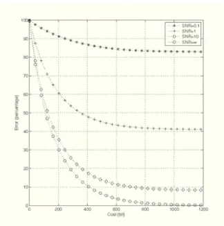
Fig. 2. Experiment 1: Errorvs.costfor different values of SNR.N=256,

M = 256, a = 0.5, SNR variable. The vertical axis is percentage error

100£(T)/tr(Kf).

Further information on the FRT and its computation may be

found in [3], [23], [24]. The system matrix H is taken to be the Nby Nrealequivalent of the N/2 by N/2 complexFRT

matrix [23]. In experiments, we have used randomly chosen

covariance matrices Kf and Kn, and defined a parameter

SNR A tr(HKfHT)

SR=tr(Kn)

tr(Kf)

tr(Kn) (16)

(Equivalence of thetwoforms is duetoorthonormality of real FRT matrices, HTH = I.) SNR measures the ratio of signal

power to inherentsystem noisepower, before measurements.

To obtain the trade-off curve between the MSE error £(Q)

andmeasurement cost Q, thealgorithm of Section V has been

used. The cost j3 is measured in bits by taking logarithms to

base 2.

Experiment 1: In this experiment, the FRT orderwas fixed

as a = 0.5, with N = M = 256. SNR was variable,

ranging over 0.1, 1, 10 and oc. The computed £(Q) vs. 3

curves are presented in Fig. 2. We notice that (S3) is very

sensitivetoincreasesin for smallenough Q,then itbecomes

less responsive and eventually saturates at the asymptote for infinite measurement accuracy.

We haverepeated the above experiment forseveral different

values of the FRTordera. Theresulting trade-offcurves were

nearly indistinguishable from the ones in Fig. 2, although the

distribution ofcost among the measurement devices changes with a.This indicates that the MSE is notcritically dependent

on how far the measurement devices are placed along the

propagation axis, which is not surprising since the field that

we are trying to reconstruct undergoes a reversible unitary

transformation as it propagates, withoutpicking up additional

noise due to propagation effects such as turbulence in the

atmosphere. Had the model included such effects, we would

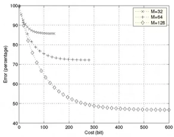
MM32 M=64 M=128 I'l 70 6 LU60 0 50 -40' 0 100 200 300 Cost(bit) 400

Fig. 3. Experiment 2: Error vs. costfor N = 256, a

M=32,64, 128variable.

6 500 600

0.5, SNR=10,

expect a degradation of the trade-off curves as measurements are made atincreasing distances. This subject is left for future

work.

Experiment 2: This experiment investigates thedependence of£(Q) for afixedQonM.Fig. 3 shows theresultfor a= 0.5,

N = 256, SNR= 10, andM = 32,64,128.The measurement

locations were chosen from a uniform grid and the grid for M= 32 was a sub-grid of that for M =64 which was a

sub-grid of that for M = 128. We see that for low values of cost,

added degrees of freedom for measurement locations doesnot significantly improve performance. However, as the allowed

cost is increased, the benefit of spreading the measurement devices to more locations becomes significant. This example

illustrates the importance of the structural problem in which

the main task is to determine the number and locations of the

measurement devices. Clearly, one may attack the structural problem by solving multiple carefully chosen instances of the metrical problem; however, a more methodical approach is desired and left as a subject for future study.

VII. CONCLUSION

We have given a precise formulation of the measurement problem for estimation of scalar wave fields in an optical

context; the formulation has information-theoretic as well as

estimation-theoretic elements. The formulation is also general

enough to be applicable in other areas where one wishes to

estimate the input of a linear system using noisy

measure-ments. The novelty of the estimationproblem here stems from

two elements specificto this problem: (i) allowing the number

and location of measurement devices to be variable, (ii) the

assignment of costs to measurements. We have pointed out

the close connection of the measurementproblem to the

rate-distortion problem, and also the essential differences between

them. A numerical algorithm has been given which rapidly

determines the trade-off betweenmeasurement cost and

mean-square error.The numerical examples showed theapplicability

of the method to problems of interest in optics and have

revealed quantitative trade-offs that were readily interpretable

in an optical context. The structural problem, in which the

numberandlocations of the probesaresubjecttooptimization,

is an interesting openproblem left for future study.

ACKNOWLEDGEMENT

This work was supported in part by TUIBITAK grant

EEEAG-105E065. Additionally,H. M. Ozaktas was supported

in part by the Turkish Academy of Sciences.

REFERENCES

[1] L. Onuraland H. M. Ozaktas, "Signal processing issues in diffraction and holographic 3dtv," Signal Processing: Image Communication, in print.

[2] M. J. Bastiaans, "Applications ofthe Wigner distribution function in optics," inThe WignerDistribution: Theory and Applications in Signal Processing, W. Mecklenbraukerand F. Hlawatsch, Eds. Amsterdam: Elsevier, 1997, pp. 375-426.

[3] H. M.Ozaktas, Z. Zalevsky, and M. A. Kutay, The Fractional Fourier Transform with Applications in Optics and Signal Processing. New York:Wiley, 2001.

[4] W. Lukozs, "Optical systems with resolving powers exceeding the classical limit," Journal of the Optical Society of America, vol. 56, no. 11, pp. 1463-1472,November 1966.

[5] G. Toraldo Di Francia, "Resolving power andinformation,"Journalof the Optical Society of America, vol.45,no.7, pp.497-501, July 1955. [6] ,"Degrees offreedom of an image," Journal of the Optical Society

of America,vol.59,no.7, pp. 799-804, July 1969.

[7] F. Goriand G. Guattari, "Effects ofcoherenceonthe degreesoffreedom of animage," Journal of theOpticalSocietyofAmerica, vol. 61,no. 1, pp. 36-39, January 1971.

[8] ,"Degrees offreedom of images from point-like-element pupils," JOSA, vol.64, no. 4, pp. 453-458, April1974.

[9] R.Piestunand D. A. Miller, "Electromagneticdegrees offreedomof an opticalsystem," Journal of the OpticalSocietyofAmericaA, vol. 17, no. 5, pp. 892-902, May 2000.

[10] D. MacKay,"Quantal aspects ofscientific information,"IEEE Transac-tions onInformation Theory, vol. 1,no. 1,pp.60-80,February 1953. [11] J. T. Winthrop, "Propagation of structural information in optical wave

fields," Journalof the Optical Society ofAmerica, vol. 61, no. 1, pp. 15-30, January 1971.

[12] D.Gabor, "Light andinformation," in Progress In Optics, E.Wolf, Ed. Elsevier, 1961, vol. I, ch.4, pp. 109-153.

[13] L.Onural, "Sampling ofthediffraction field," AppliedOptics,vol. 39, no. 32, pp. 5929-5935, November2000.

[14] F. T. Yu, EntropyandInformation Optics. New York: MarcelDekker, 2000.

[15] R. Barakat, "Some entropic aspects of optical diffraction imagery," OpticsCommunications, vol. 156,no.6,pp.235-239, November 1998. [16] P.Refregier andJ. Morio, "Shannonentropyofpartiallypolarized and partially coherent light with Gaussian fluctuations,"JOSAA, vol. 23, no. 12, pp. 3036-3044,December2006.

[17] A. Stern andB. Javidi, "Shannon number andinformationcapacityof three-dimensional integralimaging,"Journal ofthe OpticalSociety of America A,vol. 21, no. 9, pp.1602-1612, September2004.

[18] R. G.Gallager, InformationTheoryand Reliable Communication. New York: Wiley, 1968.

[19] R. V. L. Hartley, "Transmission ofinformation," Bell System Technical Journal,vol. 7, pp. 535-563, July1928.

[20] C. E. Shannon, "A mathematical theory of communication," BSTJ, vol. 27,pp.379-423 and623-656, July and October 1948.

[21] B. M.Oliver, J. R. Pierce,andC. E.Shannon, "ThephilosophyofPCM," inProceedingsof the I.R.E., vol. 36, November 1948,pp. 1324-1331. [22] H. M. Ozaktasand D.Mendlovic, "Fractional Fourieroptics," Journal

oftheOpticalSocietyofAmericaA,vol. 12,no.4,pp. 743-751, April 1995.

[23] oC. Candan, M. A. Kutay,andH. M. Ozaktas, "The discrete fractional Fourier transform,"IEEE Transactions on SignalProcessing, vol. 48, no. 5,pp. 1329-1337, May 2000.

[24] H. M. Ozaktas, 0. Arikan, M. A. Kutay, and G. Bozdagi, "Digital computationofthefractional Fouriertransform,"IEEETransactionson