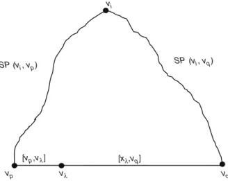
Research & Management Science
Volume 155
Series Editor Frederick S. Hillier
Stanford University, CA, USA Special Editorial Consultant Camille C. Price
Stephen F. Austin State University, TX, USA This book was recommended by Dr. Price
For further volumes:
Editors
Foundations of Location
Analysis
ISSN 0884-8289
ISBN 978-1-4419-7571-3 e-ISBN 978-1-4419-7572-0 DOI 10.1007/978-1-4419-7572-0
Springer New York Dordrecht Heidelberg London
© Springer Science+Business Media, LLC 2011
All rights reserved. This work may not be translated or copied in whole or in part without the written permission of the publisher (Springer Science+Business Media, LLC, 233 Spring Street, New York, NY 10013, USA), except for brief excerpts in connection with reviews or scholarly analysis. Use in con-nection with any form of information storage and retrieval, electronic adaptation, computer software, or by similar or dissimilar methodology now known or hereafter developed is forbidden.
The use in this publication of trade names, trademarks, service marks, and similar terms, even if they are not identified as such, is not to be taken as an expression of opinion as to whether or not they are subject to proprietary rights.
Cover design: eStudioCalamar S.L. Printed on acid-free paper
Springer is part of Springer Science+Business Media (www.springer.com)
University of New Brunswick Faculty of Business Administration Fredericton, New Brunswick Canada
Pontificia Universidad Católica de Chile Depto. Ingenieria Electrica
Av. Vicuna Mackenna 4860 Macul, Santiago
Chile
nail jelly to the wall.
vii
This book is the final result of a number of incidents that occurred to us while discussing location issues with colleagues at conferences. Frequently we attended presentations, in which the authors quoted the well-known references that helped to make the discipline what it is today. Upon further inquiry, though, it turned out that some of these colleagues had never actually read the original papers. We then discussed among ourselves which contributions could be credited with shaping the field. And, lo and behold, we found that we, too, had neglected to read some of the papers that form the foundation of our science. Whether it was laziness or other things that got in the way, it had become clear that something had to be done.
Our first thought was to collect the original contributions (once we could agree on what they were) and reprint them. When discussing this possibility with a pub-lisher, we immediately ran into a roadblock in the form of copyright. While this appeared to have stopped our enthusiastic effort dead in its tracks, we kept on col-lecting and reading what we considered original contributions.
This went on until we met Camille Price, who suggested that, rather than reprint-ing the original contributions, we should invite some of the leaders in our field and ask them to describe the original contribution, explain and interpret it, and comment on the impact that it had to the field. This was, of course, an excellent idea, and the response by our colleagues to our pertinent requests was equally enthusiastic. What you hold in your hands is the result of this effort.
In other words, the purpose of this book is to provide easy access to the main contributions to location theory. The book is organized as follows. The introductory chapter provides an overview of some of the many facets of location analysis. This is followed by contributions in the main three fields of inquiry: minisum, mini-max, and covering problems. The next chapters are part of an ever-growing list of nonstandard location models: models including competitive components, those that locate undesirable facilities, those with probabilistic features, and those that allow interactions between facilities. The following chapters discuss solution techniques: after a discussion of exact and heuristic techniques, we devote an entire chapter to Weiszfeld’s method, and another to Lagrangean techniques. The last chapters of this book deal with the spheres of influence that the facilities generate and that attract
customers to them, and the last chapter delves back into the origins of location sci-ence, when geographers discussed central places.
Since the book is written by different individuals, the style and notations differ. Initial attempts to unify the notation were nipped in the bud. It is apparent that some chapters will be accessible to the laymen, others require substantial mathematical knowledge. However, all are written by competent individuals, who have made a major effort to not only popularize the original work, but also to assess its impact on the field and its implications for theory and practice.
With great sadness we have to report the untimely death of one of our contribu-tors, Professor Roberto Galvão. His chapter is certainly one of the highlights of this book. In order to publish his contribution, it was required to have the usual consent form signed by a relative of his. Alas, none was to be found. Since we are certain that it would have been Professor Galvão’s will to see his work in print, Professor Marianov now formally appears as coauthor (and, as such, being able to sign the necessary form), while the chapter was and remains entirely that of Roberto.
Last, but certainly not least, it is our great pleasure to thank all individuals who have contributed to this work and helped to make it reality. First and foremost, there are the contributors to this volume, who have devoted their time and talents to the cause of making the original contributions in our field accessible to those interested in the area. Then, of course, there is Camille Price, without whose suggestions and encouragement this book would never have seen the light of day. Thanks also go to Professor Hillier for his patience, and to Mr. Amboy for his timely help with the preparation of a camera-ready copy of the manuscript.
H. A. Eiselt Vladimir Marianov
ix
Part I Introduction ... 1 1 Pioneering Developments in Location Analysis ... 3
H. A. Eiselt and Vladimir Marianov
Part II Minisum Problems ... 23 2 Uncapacitated and Capacitated Facility Location Problems ... 25
Vedat Verter
3 Median Problems in Networks ... 39
Vladimir Marianov and Daniel Serra
Part III Minimax Problems ... 61 4 Continuous Center Problems ... 63
Zvi Drezner
5 Discrete Center Problems ... 79
Barbaros Ç. Tansel
Part IV Covering Problems ... 107 6 Covering Problems ... 109
Lawrence V. Snyder
Part V Other Location Models ... 137 7 Equilibria in Competitive Location Models ... 139
H. A. Eiselt
8 Sequential Location Models ... 163
9 Conditional Location Problems on Networks and in the Plane ... 179
Abdullah Dasci
10 The Location of Undesirable Facilities ... 207
Emanuel Melachrinoudis
11 Stochastic Analysis in Location Research ... 241
Oded Berman, Dmitry Krass and Jiamin Wang
12 Hub Location Problems: The Location of Interacting Facilities ... 273
Bahar Y. Kara and Mehmet R. Taner
Part VI Solution Techniques ... 289 13 Exact Solution of Two Location Problems via Branch-and-Bound .... 291
Timothy J. Lowe and Richard E. Wendell
14 Exploiting Structure: Location Problems on Trees and
Treelike Graphs ... 315
Rex K. Kincaid
15 Heuristics for Location Models ... 335
Jack Brimberg and John M. Hodgson
16 The Weiszfeld Algorithm: Proof, Amendments, and Extensions ... 357
Frank Plastria
17 Lagrangean Relaxation-Based Techniques for Solving
Facility Location Problems ... 391
Roberto D. Galvão and Vladimir Marianov
Part VII Customer Choice And Location Patterns ... 421 18 Gravity Modeling and its Impacts on Location Analysis ... 423
Lawrence Joseph and Michael Kuby
19 Voronoi Diagrams and Their Uses ... 445
Mark L. Burkey, Joy Bhadury and H. A. Eiselt
20 Central Places: The Theories of von Thünen, Christaller,
and Lösch ... 471
Kathrin Fischer
xi
Oded Berman Rotman School of Management, University of Toronto,
105 St. George Street, Toronto, ON M5S 3E6, Canada e-mail: [email protected]
Joy Bhadury Bryan School of Business and Economics,
University of North Carolina – Greensboro, Greensboro, NC 27402-6170, USA e-mail: [email protected]
Jack Brimberg Department of Mathematics and Computer Science,
Royal Military College of Canada, Kingston, ON K7K 7B4, Canada e-mail: [email protected]
Mark L. Burkey School of Business and Economics,
North Carolina A & T State University, Greensboro, NC, USA e-mail: [email protected]
Abdullah Dasci School of Administrative Studies, York University,
4700 Keele Street, Toronto, ON M3J 1P3, Canada e-mail: [email protected]
Zvi Drezner Steven G. Mihaylo College of Business and Economics,
California State University-Fullerton, Fullerton, CA 92834, USA e-mail: [email protected]
H. A. Eiselt Faculty of Business Administration, University of New Brunswick,
Fredericton, NB E3B 5A3, Canada e-mail: [email protected]
Kathrin Fischer Institute for Operations Research and Information Systems
(ORIS), Hamburg University of Technology, Schwarzenbergstr. 95, 21073 Hamburg, Germany
e-mail: [email protected]
Roberto D. Galvão COPPE, Federal University of Rio de Janeiro,
John M. Hodgson Department of Earth and Atmospheric Sciences,
The University of Alberta, Calgary, AB T6G 2R3, Canada e-mail: [email protected]
Lawrence Joseph School of Geographical Sciences and Urban Planning,
Arizona State University, Tempe, AZ 85287-0104, USA e-mail: [email protected]
Bahar Y. Kara Department of Industrial Engineering, Bilkent University,
Ankara, Turkey
e-mail: [email protected]
Rex K. Kincaid Department of Mathematics, The College of William and Mary,
Williamsburg, VA 23187-8795, USA e-mail: [email protected]
Dmitry Krass Rotman School of Management, University of Toronto,
105 St. George Street, Toronto, ON M5S 3E6, Canada e-mail: [email protected]
Michael Kuby School of Geographical Sciences and Urban Planning,
Arizona State University, Tempe, AZ 85287-0104, USA e-mail: [email protected]
Timothy J. Lowe Tippie College of Business, University of Iowa, Iowa City,
IA 52242-1994, USA
e-mail: [email protected]
Vladimir Marianov Department of Electrical Engineering, Pontificia
Universidad Católica de Chile, Santiago, Chile e-mail: [email protected]
Emanuel Melachrinoudis Department of Mechanical and Industrial
Engineering, Northeastern University, 360 Huntington Avenue, Boston, MA 02115, USA
e-mail: [email protected]
Frank Plastria Department of Mathematics, Operational Research, Statistics
and Information Systems for Management, MOSI, Vrije Universiteit Brussel, Pleinlaan 2, B1050 Brussels, Belgium
e-mail: [email protected]
Daniel Serra Department of Economics and Business, Pompeu Fabra University,
Barcelona, Spain
e-mail: [email protected]
Lawrence V. Snyder Department of Industrial and Systems Engineering, Lehigh
University, 200 West Packer Ave., Mohler Lab, Bethlehem, PA 18015, USA e-mail: [email protected]
Mehmet R. Taner Department of Industrial Engineering, Bilkent University,
Ankara, Turkey
e-mail: [email protected]
Barbaros Ç. Tansel Department of Industrial Engineering, Bilkent University,
6800 Bilkent, Ankara, Turkey e-mail: [email protected]
Vedat Verter Desautels Faculty of Management, McGill University, Montreal,
Quebec, Canada
e-mail: [email protected]
Jiamin Wang College of Management, Long Island University,
720 Northern Blvd., Brookville, NY 11548, USA e-mail: [email protected]
Richard E. Wendell Joseph M. Katz Graduate School of Business,
University of Pittsburgh, Pittsburgh, PA 15260, USA e-mail: [email protected]
Hassan Younies School of Management, New York Institute of Technology,
Abu Dhabi, United Arab Emirates e-mail: [email protected]
3
1.1 Location Problems: Its Problem Statement,
Its Components, and Applications
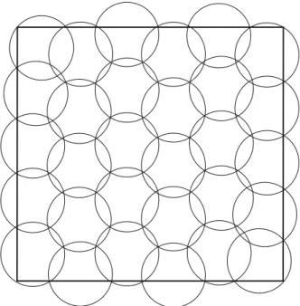
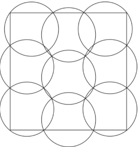
A mathematician would probably define a location problem as solving the follow-ing question: “given some metric space and a set of known points, determine a num-ber of additional points so as to optimize a function of the distance between new and existing points.” A geographer’s explanation might be that “given some region in which some market places or communities are known, the task is to determine the sites of a number of centers that serve the market places or communities.” Students of business administration will want to determine “the location of plants and market catchment areas in the presence of potential customers,” while computer scientists (or, more specifically, analysts in computational geometry) may want to determine “the minimum number of equal geometrical shapes that are required to cover a cer-tain area, and the positions of their centroids.”
All these views have in common the basic components of a location problem: a space, in which a distance measure is defined, a set of given points, and candidate locations for a fixed or variable number of new points. We refer to the known points as “customers” or “demands,” and the new points to be located as “facilities.”
As far as the space is concerned in which customers are and facilities are to be lo - cated, we distinguish between a subset of the d-dimensional real space (most promi-nently, the two-dimensional plane) and networks. Each of these two categories has two subcategories: one, in which the location of the facilities is continuous, and the other, in which it is discrete. These two subcategories will determine the toolkit needed by the researcher to solve problems. In discrete problems, the decision is
H. A. Eiselt, V. Marianov (eds.), Foundations of Location Analysis, International Series in Operations Research & Management Science 155,
DOI 10.1007/978-1-4419-7572-0_1, © Springer Science+Business Media, LLC 2011
Pioneering Developments in Location Analysis
H. A. Eiselt and Vladimir MarianovH. A. Eiselt ()
Faculty of Business Administration, University of New Brunswick, Fredericton, NB E3B 5A3, Canada
e-mail: [email protected] V. Marianov
Department of Electrical Engineering, Pontificia Universidad Católica de Chile, Santiago, Chile
whether or not to locate a facility at that spot, thus modeling the decision with a binary variable is obvious. The result is a (mixed-)integer linear programming prob-lem. On the other hand, continuous problems will have continuous variables asso-ciated with them, indicating the coordinates of the facilities that are to be located. Since functions of the distance are typically nonlinear, a nonlinear optimization problem will follow in this case. With the tools for the solution of the different types of problems being so different, it is little surprise that most researchers have decided to either work with continuous or with discrete models. Both types of models are represented in this book.
The space commonly corresponds to a geographical region. An obvious choice for representing such a region is the two-dimensional plane. In some cases, a one-dimensional space is a used to simplify the analysis of complicated problems, as in the case that includes competition between firms. Location problems can also be defined over non-geographical spaces. For example, an issue space in which potential voters for a presidential election are located according to their positions in relation to the issues. The problem would be to optimally locate a candidate so to maximize his vote count in the presence of competing candidates, assuming that voters will vote for the candidate whose position is closest to them. Or consider a skill space in which a number of tasks (demands) have known locations, each loca-tion representing the combinaloca-tion of skills required to successfully accomplish the task. The location problem would be to locate company employees in such a way that all tasks are performed by sufficiently skilled employees, and no employee is overloaded with work.
In this book we deal with location problems, which are defined as models, in which the facilities and demands are very small as compared to the space they are located in. Examples of facility location problems are finding the location of an assembly plant within a country; or selecting the site of a school in one of several candidate points in a city. In these cases, the facilities can be considered dimension-less points. A generalization would be the location of lines in a plane, where the lines represent a new road. In some cases, location problems can be cast as geo-metrical problems: an example is finding the smallest circle that contains a known set of points on a plane, which is equivalent to locating a facility (the center of the circle) in such a way that the largest distance (the radius of the circle) between any customer (the given points) and the facility (the center of the circle) is minimized. In contrast to location problems, layout problems feature facilities, whose size is significant in comparison to the space the facility is to be located in. Examples of layout problems include the siting of a drilling machine in a workshop, the location of tables in a fast-food restaurant, or the location of supply rooms in a hospital. Other things being equal, layout problems are more difficult than location problems with similar features. One reason is that layout problems must consider the shape of the facility to be located, which is unnecessary in location models, where facilities are just points. Layout models are not discussed in this book.
Location problems can be formulated to answer to several different questions. Not only can the location of the facilities be unknown, but also the number of fa-cilities and their capacities. Furthermore, when there is more than one facility, the solution of the location problem also requires finding the assignment of demands to
facilities, called the “allocation” problem. Examples of this problem are the assign-ment of individual customers to a particular warehouse from which grocery is to be delivered by a phone-order company, or the dispatching of specific ambulances to emergency sites. In these cases, the owner or operator of the facilities does the al-location, but there are other cases in which users decide what facility to patronize, such as the decision which theater to patronize or at what fast-food store to have lunch.
For the location problem to make sense, customers and facilities must be related by distance. Again, this distance can be measured either over a geographical region or over any kind of space. Typical goals are to minimize the distance between fa-cilities and their assigned customers (minisum problems) or maximize the amount of demand (number of customers) that is within a previously specified distance from their assigned facilities. When all the demand is to be served, a goal could be to minimize the number of facilities needed for all the customers to be within a distance from their facility. If competing facilities are involved and distance is an issue for customers, the planner’s objective will be to locate his facilities closer than competitors’ facilities to as many customers as possible.
Proximity to facilities is, however, not always desirable. When locating a new landfill, most people will object if the facility is to be located close to their homes— the usual NIMBY (not in my back yard) argument applies, even though they usu-ally understand that locating the landfill too far away will cost them, as they are, directly or indirectly, charged for the collection and transportation costs of the solid waste. In this case, the problem could be formulated with conflicting objectives: the landfill should be not too far from the area it serves, but most of the population should be as far as possible from it. These objectives have been described as “push” and “pull”.
Besides distances between facilities and demands, there are other factors that can be relevant when seeking good locations. Availability of services and skilled tech-nicians at the candidate locations, land cost, existence of competitors and regional taxes are some examples. While such factors are maybe as important as or possibly even more important than proximity, most standard location problems do not con-sider them. This stresses the importance of concon-sidering the output of the standard location models as an input for the decision maker, who can then include any of the features that were ignored by the mathematical model.
Most of the applications of location models involve, decisions on the strate-gic level. As such, the decisions tend to be long-term, which implies that many of the data used in the decision-making process, will be quite uncertain. While there usually are few changes concerning distances, future demand tends to be highly uncertain. This problem is exacerbated by the high cost of locating and relocating a facility, meaning that once a location is chosen, it can only be changed at great ex-pense. This argument implies that probabilistic and/or robust models are most likely to result in facility locations that are acceptable to decision makers.
Applications of location models are found in many different fields. Some of these applications are fairly straightforward, such as the locations of trucking ter-minals, blood banks, ambulances, motels and solid waste transfer points. Others are nontraditional and not at all obvious. Good examples are the location of measuring
points for glaucoma detection, the location of new employees in skill space, the location of advertisements in media and many others.
1.2 A Short History of the Early Developments
in Location Analysis
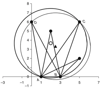
In the early seventeenth century, a question was posed about how to solve the fol-lowing puzzle: “Given three points in a plane, find a fourth point such that the sum of its distances to the three given points is as small as possible.” This question is credited to Fermat (1601–1665), who used to tease his contemporary mathema-ticians with tricky problems. The earliest (geometrical) solution is probably due to Torricelli (1598–1647), Fermat’s pupil and the discoverer of the barometer, al-though due to the many discoveries and rediscoveries of the problem and its solu-tion, there are different opinions about the true origin of the problem and who solved it first. Because of the many scientists involved in the process, the problem has been called the Fermat problem, the Fermat-Torricelli problem, the Steiner problem, the Steiner-Weber problem, the Weber problem, and many variation thereof. The inclu-sion of Weber’s name follows his generalization of the problem by assigning dif-ferent weights to the known points, so transforming the mathematical puzzle into an industrial problem, in which a plant is to be located (the unknown point) so to minimize transportation costs from suppliers and to customers (the known points) requiring different amounts of products (the weights). Weber’s name stuck, even though the formulation of the model in Weber’s book is in an appendix written by Pick. Even if the first formal occurrence of a location problem were due to Fermat or one of his contemporaries, location analysis must be much older than that. For centuries before, people may have wondered in which cave to live, where to build houses, villages, churches, and other “facilities.” And they solved these problems using some sort of heuristic method.
Location problems frequently require solving an associated allocation or assign-ment problem: if locations for more than one facility are known, which facility will serve what customers? A step towards the solution of the allocation problem was taken very early in the seventeenth century. Descartes imagined the universe as a set of vortices around each star—the “heavens”—and illustrated his theory with a drawing that made an informal use of what later would become known as Voronoi polygons and Voronoi diagrams. This concept was subsequently used by Dirichlet in 1850, extended to higher dimensions by Voronoi and rediscovered by Thiessen, both in the early twentieth century. While Thiessen’s application involves an im-proved estimate of precipitation averages, Voronoi diagrams are generally useful tools when consumers have to be assigned to their closest facilities.
Between the 1600s and the 1800s, there was no registered activity related to location problems other than a puzzle in the Ladies Diary or Woman’s Almanack in 1755 as reported in a book edited by Drezner and Hamacher in 2002. In 1826, the geographer von Thünen developed a theory concerning the allocation of crops on the land that surrounds a town. His point was that the agricultural activity should
be organized around the town according to transportation costs and value of the products. This theory results in crops cultivated in concentric circles about the town. Clearly, a location issue, although it could also be considered a land layout problem, as the areas or rings to be located around the central place are sizeable in compari-son to the space considered.
In 1857, Sylvester asked another location-related question: “It is required to find the least circle which shall contain a given system of points in a plane.” This ques-tion was later answered by Sylvester himself in 1860 and by Chrystal in 1885. Nowadays, we would call this a one-center problem in the plane.
As in many other fields, the pace of discoveries increased dramatically in the twentieth century. In the late 1920s, the mathematical statistician-turned economist Hotelling wrote a seminal paper on competitive location models that spawned a rich diversity of models that are still under active discussion today. Also during that time, Reilly introduced gravity models into the fray as a way customers gravitate to facilities The 1930s saw contributions by Christaller, who founded central place theory, and Weiszfeld, who developed his famed algorithm that solved Weber prob-lems with an arbitrary number of customers.
Later important contributions included those by Lösch and the regional scientists Isard and Alonso. The birth of modern quantitative location theory occurred in the mid-1960s, when Hakimi wrote his path-breaking analysis of a location model on networks, which, in today’s parlance, is a p-median problem. Following Hakimi’s papers, ReVelle, Church, Drezner, Berman, and many others have made important contributions to location science. Some of those have also contributed to this book.
1.3 Some Standard Location Problems
Facility location problems can take a variety of forms, depending on the particular context, objectives and constraints. It is common to classify location problems in minisum, covering and minimax problems. Most of the numerous remaining facil-ity location problems can be seen as combinations or modified versions of these key problems. We present here prototypes of these basic classes, as well as an as-sortment of other models that we consider of importance, either from a theoretical viewpoint, or because of their practical interest. This list of models is also a guide for understanding the following chapters and a way to introduce some standard notation, since in most of the chapters of this book, the original notation of the re-viewed papers is preserved.
We first state a base formulation, which is used throughout this section to present some of the different problems and models for location on networks. This formula-tion applies only when demands lie at the nodes and facilities are to be located only at nodes of the network. The problem can be formulated as follows.
(1.1) Min σ i,j cijyij + j fjxj + gz
(1.2)
(1.3) (1.4) where the variables are:
xj: a location variable that equals 1, if a facility is located at node j, and 0 otherwise,
yij: an allocation variable that equals 1, if customer i is assigned to a facility at j, and 0 otherwise, and
z: a continuous variable that takes the value of a maximum or a minimum
dis-tance, depending on the problem being solved. The subscripts are
i, j: a subscript that indicates customers and potential facility sites, respectively, Ni: is the set of nodes. Its definition depends on the problem, and n and m denote
the total number of customers and potential facility locations, respectively. Finally, the parameters are
: a parameter that takes the value 1 or (−1), depending on whether the
objective is minimized or maximized, and
cij, fj, g: parameters that depend on the problem being solved.
The objective (1.1) of the base problem optimizes linear combinations of the loca-tion and allocaloca-tion variables and the distance variable. Depending on the problem, these linear combinations represent maximum, minimum or average distances, in-vestment or transportation and manufacturing costs. The set of constraints (1.2) state that each customer’s demand must be satisfied, and that all of it is satisfied from one facility. In other words, that each customer or demand node is assigned to or served by exactly one facility. The set of constraints (1.3) allows demand node
i to be assigned or allocated to a facility at j only if there is an open facility in that
location i.e., xj = 1. Constraints (1.4) define the nature of all variables as continuous or binary. Note that these constraints define a feasible set of solutions of the prob-lem of locating a (yet) undetermined number of facilities, choosing their sites from a number of known candidate locations, and finding the right assignment of demand nodes or customers to these facilities.
1.3.1 Minisum Problems
Minisum problems owe their name to the fact that a sum of facility-customer dis-tances is minimized. These problems include single-facility, multiple-facility and
s.t.
j∈Ni
yij = 1 i = 1, 2, . . . n
yij ≤ xj i= 1, 2, . . . n, j = 1, 2, . . . m.
weighted versions of the Weber problem; the simple plant location problem SPLP and the p-median problem PMP.
1.3.1.1 Minisum Problems on the Plane: The Weber Problem
The Weber problem consists in finding the coordinates ( x, y) of a single facility X that minimizes the sum of its distances to n known customer or demand points with coordinates ( ai, bi) and weights wi, i = 1, 2, … n, all of them lying on the same plane. This is an unconstrained nonlinear optimization problem, and its general formula-tion is
where d( X, Pi) is the distance between the facility and demand i. If Euclidean dis-tances are used, this distance is d(X, Pi)=
(x− ai)2+ (y − bi)2.
An application of this problem is locating a single warehouse (the facility) that supplies different amounts (weights) of products to a number of dealers (the de-mands), in such a way that the total transportation cost is minimized, assuming that this cost depends on the distance and amount of transported product.
The solution of this problem is easily found using differential calculus. However, the coordinates of the optimal facility location turn out to be a function of the dis-tance d( X, Pi), which is unknown. The practical solution of this problem, found by Weiszfeld, involves the use of an iterative algorithm that takes as an initial solution the point that minimizes the sum of the squares of the distances.
A natural generalization of the Weber problem is its multiple-facility version. As more than one facility is to be located, an allocation problem must be solved together with the location problem, which makes the problem far more difficult. In the simplest case, the assumption is made that each demand is assigned to its closest facility. This problem was described and a heuristic proposed by Cooper in 1963.
1.3.1.2 Minisum Problems on Networks: Plant Location and Median Problems
The Simple Plant Location Problem
The simple plant location problem, sometimes also referred to as the uncapacitated
facility location problem seeks minimizing production, transportation and
site-relat-ed investment costs. The model assumes that the costs of opening the facilities de-pend on their location, and that the investment budget is not a constraint. Then, the number of facilities to be opened is left for the model to decide. Its integer program-ming formulation is the base model (1.1)–(1.4), with σ = +1, cij = (ej+ ˜cijdij)wi,
Min z(X)=
n
i=1
where ej denotes the production cost per unit, ˜cij are the transportation costs from
node i to j per unit, dij symbolizes the shortest distance between i and j, the param-eters wi denote the quantity of the product that must be shipped to customer i, the parameters fj are the fixed costs of opening a facility at node j, and g equals zero. The set Ni in constraints (1.2) contains all possible candidates to location of facili-ties. The objective to be minimized, representing the total sum of variable and fixed costs, is now:
Since the costs of locating facilities are included in the objective, the solution of the model prescribes the number of facilities to be located, depending on the tradeoff between transportation and fixed costs.
There is also a “weak” formulation of this problem that uses an aggregated ver-sion of constraints (1.3) for each facility location j,
jyij ≤ nxj.
There is an important body of literature focusing on this problem, because of its versatility and practical interest. Due to its difficulty, many solution methods have been proposed. In Chap. 2 of this book, Verter describes this problem, and reviews in detail the classical dual ascent method by Erlenkotter, as well as the heuristic proposed by Kuehn and Hamburger.
The 1-Median Problem
The network equivalent of the single-facility Weber problem on the plane is the 1-median problem, whose formulation is exactly the same as that of the single-facility Weber problem. However, in the 1-median problem the demands occurs at the nodes of a network. Hakimi proved that there is always an optimal location of the facility at a node of the network. As a consequence, finding the solution reduces to searching the nodes of the network, and the problem can be stated as follows: find a node v* such that for all nodes v
k, k = 1, 2, … n,
This problem has been solved for locations on tree networks in the 1960s by Hua-Lo Keng, who was looking for the optimal location of a threshing floor for wheat fields, and rediscovered by Goldman in 1971.
The p-Median Problem
The p-median problem is a p-facility generalization of the 1-median problem, in which it is assumed that the decision maker knows how many facilities are to be
lo-Min i,j cijyij + j fjxj. n i=1 wid(v∗, vi)≤ n i=1 wid(vk, vi).
cated, and that the cost of locating the facilities is the same no matter where they are located. As in the continuous case, the allocation problem must be solved together with the location problem, i.e., not only the location of the p facilities needs to be found, but also, for each demand, the facility to which this demand is assigned. Let
Xp be a set of p points x1, x2, … xp. Define distance of a node vi to its closest point in Xp as
Then the set Xp* is a “p-median” of the network, if for every X
p on the network,
i.e. Xp* is the set of p points on the graph such that, if facilities are open at these
points, the total weighted distance between the demands and their closest facility would be minimized. For this problem, Hakimi proved that there is always a solu-tion set containing only nodes of the network.
ReVelle and Swain formulated this problem as a linear integer programming problem. Their model uses the same equations (1.1)–(1.4) of the basic formula-tion above, and an addiformula-tional constraint that requires exactly p facilities to be located:
In their formulation of the p-median, the objective minimizes the sum of the weight-ed facility-demand distances, i.e., in the objective (1.1) of the basic formulation, the parameters become σ = +1, cij = widij, where wi is the weight associated to
each demand node (demand volume or number of customers) and dij is the shortest distance between nodes i and j, measured along routes on the network, fj = 0, and
g = 0. The objective (1.1) becomes
Also, the set Ni in constraint (1.2) contains all possible candidates to location of facilities. Note that this formulation assumes that each demand is assigned to its closest facility.
In Chap. 3 of this book, Marianov and Serra review the classic contributions of Hakimi, made in 1964 and 1965, including the definitions of the absolute median and the absolute p-medians of a network. Also, they review the paper in which the first integer programming formulation of the p-median problem was proposed by ReVelle and Swain in 1970.
d vi, Xp = min d(vi, x1), d(vi, x2), ..., d(vi, xp) . n i=1 wid vi, Xp∗ ≤ n i=1 wid vi, Xp j xj = p. Min i,j widijyij.
1.3.2 Minimax Problems
The idea behind minimax problems is to minimize the longest distance between a customer and its assigned facility, expecting that a maximum equity or justice will be achieved. As before, these problems have been defined both on a plane and on a network.
1.3.2.1 Continuous Minimax Problems: Single and Multiple-Facility Center Problems on the Plane
The oldest known single-facility minimax problem was formulated by Sylvester in 1857 in a one-sentence reference. The problem consists in finding the small-est circle containing a set of given points. Finding the solution of this problem is equivalent to finding the location of the center of a circle that encloses all given points, in such a way that its radius is minimized. If a facility is located at the center of the circle, and the points represent demands, the maximum distance between the facility and a demand will be minimized. This problem is now known as the 1-cen-ter on the plane or the continuous 1-cen1-cen-ter. Several geometrical solution methods have been proposed to solve this problem, the first one due to the same Sylvester and rediscovered by Chrystal in 1885.
A natural extension of the 1-center problem is the p-center on the plane. Its for-mulation is as follows. Let Xp be a set of p points x1, x2, … xp on the plane. Define distance of a customer ci to its closest point in Xp as
Then the set Xp* is a “p-center”, if for every X
p on the plane,
In other words, Xp* is the set of p points on the plane such that, if these points were
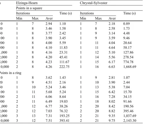
facilities, the maximum distance between a demand and its closest facility would be minimized. Minimax problems on the plane, as well as their solution methods are analyzed in Chap. 4 of this book. In that chapter, Drezner describes the early research done in the nineteenth century, shows how geometrical methods were used to solve the continuous minimax problems, describes the algorithmic contributions by Elzinga and Hearn in the 1970s, and compares both approaches through new unpublished computational experience.
1.3.2.2 The 1-Center and p-Center Problems on Networks
The 1-center on a network has been first formulated and solved by Hakimi in 1964 and the solution method improved by Goldman in 1970 and in 1972. Hakimi
for-d ci, Xp = min d(ci, x1), d(ci, x2), ..., d(ci, xp) . max d ci, X∗p = max d ci, Xp .
mulates the problem as follows: Let vi be a node, wi its potential demand, and x any point on the network. Define d( vi, x) as the minimum distance between vi and x. Find a point x* on the network such that for x,
This point is called the “absolute center” of the network. Hakimi proved that his result for minisum problems does not apply to the 1-center problem. In other words, the solution can be on an arc of the network, which is even true if all demands are equal.
Later, the 1-center was extended to a multiple-facility problem: the p-center: let
Xp be a set of p points x1, x2, … xp anywhere on the network. Define the distance between a node vi and its closest point in Xp as
Then the set Xp* is a “p-center”, if for every X
p on the network,
In other words, Xp* is the set of p points on the network such that, if these points
were facilities, the maximum distance between a demand and its closest facility would be minimized.
If facility locations are restricted to the nodes of the network, the p-center prob-lem can be formulated as an integer programming probprob-lem using the base formula-tion (1.1)–(1.4), and setting σ = +1, cij = 0, fj = 0, and g = 1. Variable z is the
maxi-mum distance between a demand and its assigned facility. Two extra constraints must be added:
(1.5) (1.6)
Constraint (1.5) requires z, the variable to be minimized, to take the value of the maximum distance between any customer and its assigned (closest) facility. Since constraint (1.2) forces assignment of each customer to exactly one facility, con-straint (1.5) can take the aggregated form
Constraint (1.6) sets the number of facilities to be located to p. Pioneering devel-opments on center problems on a network, specifically the works by Hakimi in 1964, Goldman in 1972, and Minieka in 1970 are the subject of Chap. 5 of this
max i wid(x ∗, vi)≤ max i wid(x, vi). d vi, Xp = min d(vi, x1), d(vi, x2), ..., d(vi, xp) . max i d vi, Xp ≤ max i d vi, Xp . dijyij≤ z for i= 1, 2, . . . n, j = 1, 2, . . . m, and j xj= p. j dijyij ≤ z for i= 1, 2, . . . n.
book by Tansel. The chapter first defines the single facility p-center problem and its multiple-facility version and then describes their properties. Later, the three classic contributions are reviewed: Hakimi’s definition of the absolute center, Goldman’s algorithm for locating the center and Minieka’s method for finding the p-centers on a network when locations are restricted to nodes.
1.3.3 Covering Problems
In minisum and minimax location models, the distance between each and every customer and his closest facility is explicitly considered. While minisum problems minimize the average distance between a customer and its closest facility, mini-max problems minimize the longest customer-facility distance. In contrast, covering models do not explicitly include customer—facility distances in the model and these distances only matter if they exceed a preset value D¯. A common example appears in
emergency medical services: service is considered adequate if an ambulance reaches the site of the emergency in no more than, say 8 minutes. In the food business, a piz-za parlor could offer free pizpiz-zas when the delivery time exceeds 30 minutes. In syn-thesis, the concept of coverage implies that a customer can and will be adequately served (“covered”) when a facility is located within a preset distance or travel time. Distance is no longer included in the objective function, but appears as a constraint.
1.3.3.1 The Location Set Covering Problem
The location set covering problem LSCP was first introduced by Hakimi, and
for-mulated as an integer programming problem by Toregas et al. in 1971. Its goal is to find the minimum number of facilities and their locations, so that all customers are covered, meaning that all customers are no farther than a preset distance D¯ of their
closest facility. Although the original formulation uses only location variables xj, the problem can be reformulated using the base model (1.1)–(1.4). To reproduce the
LSCP with this base model, we set σ = +1, cij = 0 ∀ i, j, fj = 1 ∀ j, g = 0, and the set
Ni in constraint (1.2) contains all candidates to location of facilities that are within distance D¯, i.e., Ni = {j : dijD¯}. The objective is now
The formulation provided by Toregas et al. is simpler. In that formulation, only location variables are used and the allocation problem is not solved, i.e. the model does not prescribe which facility provides the service, which can be provided by any of the facilities within range. In consequence, it does not matter if a customer has more than one facility within covering distance.
Min
j
Although at first sight there is no apparent relation between minimax and cover-ing problems, Minieka found that the solution of the node constrained p-center can be found by solving a sequence of location set covering problems.
1.3.3.2 The Maximal Covering Location Problem (MCLP)
If the minimum number of facilities needed to cover all the demand cannot be achieved, because of a limited budget or any other constraints on the total number of facilities, the maximal covering location problem of Church and ReVelle solves the problem of maximizing covered demand when there are a limited number of facilities to be sited. In terms of the base model (1.1)–(1.4) = − 1, cij = hi if dij ≤ D¯
and 0 otherwise, where hi is the demand volume of customer i, the fixed costs fj = 0 ∀ j, the value of g = 0, and the set Ni in constraint (1.2) contains all candidates to location of facilities. The objective is now
This objective maximizes the demand-weighted number of customers that have at least one facility located within distance D¯.
Church and ReVelle’s model was formulated using only location variables and covering variables. Again, the allocation or assignment problem is not solved by this model.
Seminal contributions on covering problems are reviewed in Chap. 6 of this book. In that chapter, Snyder thoroughly reviews the contributions by Hakimi in 1965, in which the location set covering problem is defined, the work by Toregas et al. in 1971 with the first integer programming formulation of the same problem, and the contribution by Church and ReVelle in 1974, which defines the maximum covering location problem and formulates it as an integer programming problem. The author of the chapter then adds some insight into these problems by running new computational experiments on variants of the original problems, including tradeoff between coverage and number of facilities; Lagrangean approach as a so-lution method; inclusion of budget constraints; and relationship to the p-median problem.
1.3.4 Other Relevant Location Problems
Minimax, minisum and covering models are considered the key formulations from which the remaining location problems are descendants. There are some nonstandard location problems and models that have attracted considerable atten-tion from researchers. We briefly review some of these in the remainder of this section.
Max
i,j
1.3.4.1 Competitive and Conditional Location Problems
None of the key location problems considers the existence of other facilities, either previously located or to be located in the same region by a competing firm. If this is the case, a whole new range of problems can be posed, in which the relation-ship between facilities plays an important role: competitive and conditional location problems.
In order to analyze the locational pattern of the competing firms, assumptions need to be made about consumers’ behavior. A typical assumption is that customers prefer closest facilities over more distant ones, and facilities at which the goods or service can be obtained at a lower price over the more expensive facilities.
Competitive Location: Equilibrium Problems
Suppose a market over which the demand is distributed, either continuously or at discrete points. Two firms are entering the market, each one with one facility that can move at any time without incurring costs. There are two fundamental ques-tions. The first asks that given that customers patronize the facility at which they can satisfy their demand for the lowest full price (i.e., mill price plus transporta-tion costs), is there an equilibrium? In other words, is there a situatransporta-tion, in which both facilities have decided on a location and a price, so that neither facility has an incentive to unilaterally change its price and/or its location? The second question is then, what the location and price situation in such an equilibrium is, given that it exists.
These questions—whose answer is now known as Nash equilibrium—were first answered for two competing facilities by Hotelling in 1929, who studied the prob-lem in its simplest form: a linear market (i.e., a simple line segment) with uniformly distributed customers. Each of the two firms locates a single branch, and both firms use mill pricing.
In Chap. 7, Eiselt discusses the details and applications of the problem of find-ing a locational equilibrium on a linear market; he provides a detailed review of Hotelling’s seminal paper, assesses its impact and describes subsequent work on the subject, including the article by d’Aspremont et al. Their paper was published no less than fifty years after Hotelling’s findings, and it invalidated some of Hotel-ling’s results.
Conditional Location Problems
When facilities can move freely without costs, the search for Nash equilibrium is the natural approach. However, this is not always the case. Most facilities stay where they were first located, as relocation costs are significant. If a firm is plan-ning to enter a market with immobile facilities, there are two different aspects to be considered. The first aspect concerns firms that intend to locate in the presence of
already existing competitors. this is a conditional location problems, i.e., the loca-tion of facilities, given that other facilities are already located in the region. This is the follower’s problem, who will make his location choice based on whatever profit or revenue-maximizing objective he has.
On the other hand, the already existing firms are the leaders in the location game. The leader’s problem is to locate under the consideration that after he has decided where to locate his branch(es) under the consideration that a follower will locate his own competing branches later. This means that the leader will have to take a cau-tious approach and guard against future entrants onto the market.
Solutions of this location game are usually referred to as von Stackelberg solu-tions, named after the German economist of that name. The main feature of the game is its sequential nature. In Chap. 8, Younies and Eiselt describe sequential location problems and explain the von Stackelberg concept of leader and follower firms. this is followed by a review of the classic application of these concepts in location analysis, made by Prescott and Visscher (1977), where they extend Hotell-ing results on a line to the sequential case.
In Chap. 9, Dasci discusses the conditional problems in a plane and a network, and offers a thoroughful revision of the seminal works by Drezner in 1982 and Hakimi in 1983. In these works, the follower’s problem (resulting in what is now known as an ( r|Xp)-medianoid) and the leader’s problem (dubbed an ( r|p)-centroid) are defined on the plane and a network, respectively, given that the leader locates p facilities and the follower locates r facilities.
1.3.4.2 Location of Undesirable or Semi-obnoxious Facilities
In many everyday situations, customers want to be as close as possible to the fa-cilities that are to be located. It is the case of grocery stores and shopping centers, schools, primary care centers, and similar facilities. However, the situation changes when considering facilities such as prisons, landfills, or power plants. Facilities of this nature are considered undesirable by most people. In the early days, they were referred to as noxious and obnoxious. Some people nowadays refer to these facilities as semi-obnoxious, because although nobody wants them in the neighbor-hood, they cannot be too far away, because their operation becomes too expensive. However, while realistic solutions should incorporate desirable and undesirable features in a model, undesirable facility location models push facilities as far away from customers as possible. More realistic models will have to balance some of the usual criteria (minisum, minimax, and covering) with either distance maximization (maximin or maxisum), coverage minimization, or a minimization of the costs of compensating all the affected population.
An example of a maximin formulation of undesirable facility location problems is, again, derived from the base model (1.1)–(1.4), by setting the variable z to be the minimum distance between a demand and its assigned facility, cij = 0, fj = 0, and
g = 1, and maximizing the objective, which becomes simply z. The following two
(1.7) (1.8)
Constraint (1.7) forces z to take the value of the smallest distance between a cus-tomer and his closest facility.
Early contributions on undesirable facility location are the subject of Chap. 10 by Melachrinoudis. The classical contribution of Church and Garfinkel 1978 (maxi-mizing the sum of the distances from the closest facility) is reviewed, as well as the string of papers by Shamos published in 1975, Shamos and Hoey’s work from 1975, Dasarathy and White’s paper from 1980, and Drezner and Wesolowski’s contribu-tion from 1980, all of them dealing with the maximin problem, i.e., maximizing the shortest distance between a customer and its closest facility.
1.3.4.3 Probabilistic or Stochastic Location Problems
The pool of location problems would not be complete without the consideration of uncertainty. Future demand, the time of appearance of emergency calls, service times at the facilities, and travel times between demand nodes and facilities tend to be non-deterministic. Disruptions of facilities and connecting routes are also every-day random occurrences.
There is a large body of literature dealing with problems that include one or more of these sources of uncertainty. The design of emergency services is a popular appli-cation, as well as the location of immobile facilities that can become congested. For instance, service may be refused because the facility is busy, or lines are formed in which customers have to wait until they can be served. After the 9/11 events and the destruction of New Orleans by hurricane Kathrina, many researchers have turned their attention to the location of facilities so as to mitigate such catastrophic effects, or to the search for robust locations in the sense that disruptions do not interrupt their functioning.
Chapter 11 by Berman, Krass and Wang is devoted to the description of these problems. The original contribution by Frank from 1966 is reviewed in detail, and its impact analyzed. Generalizations of Frank’s work are presented, and open prob-lems are discussed.
1.3.4.4 Hub Location Problems
Hub location problems occur mainly in transportation and telecommunications net-works. A hub is a transfer point at which either traffic from several origins is added up and forwarded to another hub, or disaggregated into several streams that are forwarded to their destination. Airlines use hub airports because they allow
tak-dijyij ≥ z i = 1, 2, . . . n, j = 1, 2, . . . m.
j
ing advantage of economies of scale, by using high capacity planes in high traffic routes, as opposed to using only small planes between every origin and destination city. Computer networks are frequently organized as a set of small hub-and-spoke networks, joined together by a backbone network.
Naturally, hub location problems have been formulated having in mind the same principles as the remaining location problems. Thus, there are p-hub location prob-lems, median-hub location probprob-lems, uncapacitated hub location probprob-lems, p-hub-center location problems, and so on. The first formulation of a hub location prob-lem by O’Kelly in 1982 was nonlinear. Later, different linearizations have been proposed. The base model (1.1)–(1.4) needs to be modified to represent an unca-pacitated hub location problem (analogous to the uncaunca-pacitated facility location problem) as follows. Facilities are now hubs, and customers need to be assigned to hubs for both their incoming and outgoing traffic. We assume each customer is as-signed to his closest hub. The traffic between two customers, hij, starts at a node i, first goes to the assigned hub k, continues from there to another hub m, and finally to the destination node j. The traffic into the opposite direction uses the same path. Both hubs could be the same, i.e., traffic could move through only one hub. We use constraints (1.2)–(1.4), but the objective is now:
(1.9) where hij is the traffic between customers or demand nodes i and j, cij is the unit traffic cost on the arc ( i, j), i.e. on the leg of the trip that goes between nodes i and
j, and is a factor <1, accounting for economies of scale. Note that the first term in
parentheses in the objective function is the cost of sending traffic from the origin to the first hub. The second term in the cost of carrying traffic between hubs, where because of the traffic concentration, it is assumed that the cost is reduced by a factor (1 − ). The third term is the cost of sending the traffic from the second hub to the destination, and the last term is the cost of opening hubs. This objective is nonlinear, but different linear versions have been proposed in the literature.
Chapter 12 of this book, written by Kara and Taner, focuses on hub location problems. O’Kelly’s seminal paper is reviewed and its contribution assessed.
1.4 An Outline of Classic Solution Methods
Most of the problems related to facility location are known to NP-hard. It is natural then to look for procedures that can find adequate optimal or approximate solutions to these problems. Many solution methods have been proposed in the literature. It is important to describe some of these methods, either because they have a broader applicability or because they led the way to the discovery of a whole line of solution procedures. This book presents some of the more important techniques.
Min i j hij k cikyik+ α k m ckmyikyj m+ m cj myj m + j fjxj
1.4.1 Exact Techniques
The best known exact solution technique for location problems written as integer programming problems is branch-and-bound. The technique was first proposed by Land and Doig in 1960. The first two contributions that apply this technique to the location field are those by Gavett and Plyter in 1966, who solve the quadratic as-signment problem, and Efroymson and Ray in 1966, who solved the uncapacitated facility location problem or, as it is frequently called today, the simple plant location problem. These two contributions are reviewed in Chap. 13 by Lowe and Wendell. The authors describe the principles behind the branch-and-bound technique, viz., partitioning the set of solution into smaller subsets, and provide a detailed descrip-tion of the two seminal papers. They also show other techniques to solve the qua-dratic assignment problem. The Efroymson and Ray approach to solving the SPLP is complemented by other branch-and-bound techniques discovered later. One sec-tion of their contribusec-tion is devoted to branching strategies.
When the problem has a special structure, as is the case when the space is a tree-shaped network, efficient techniques can be developed to find solutions to the location problems more efficiently. An example of these techniques is the method for finding the 1-median on a tree. In Chap. 14, Kincaid first defines some graph theory concepts, presents a notation for location problems, and reviews three classi-cal contributions: the Harary and Norman article of 1953, where central points on a tree are defined, the paper by Hua Lo-Keng and others in 1962—although known at an earlier date in Chinese—where the first method for location of a 1-median on a tree (and on networks with some cycles) is proposed and proven to be optimal, and the paper by Goldman in 1971, who rediscovered Hua Lo-Keng’s findings.
1.4.2 Heuristic Solution Methods
Although the maximum size of the problems that can be solved using exact meth-ods has increased in time almost like Moore’s law for semiconductors (that states that the number of transistors in an integrated chip doubles every two years), exact methods are still not capable of finding a solution in many realistic cases, in which the number of variables is too large. Heuristics are methods that find a good solu-tion, although optimality is not guaranteed or even sought. Many of these heuristics are built on principles that have been proposed a long time ago, but are still valid. Some of these, for location both in the plane and on networks, were sketched in a single paper by Cooper in 1963, and extended later by other authors. For facility location problems in the plane, a giant step forward was the heuristic for the Weber problem, which was discovered by Weiszfeld in the 1930s.
The heuristics by Cooper, and their formalization by Maranzana and by Teitz and Bart, are the subject of Chap. 15 of this book, by Brimberg and Hodgson. In that chapter, the authors describe in detail the several methods proposed by Cooper
for the continuous minisum problem, as well as the rediscoveries of these methods and their application to the discrete problem, made by Maranzana and by Teitz and Bart. Then, they assess the impact these early discoveries had, their application to other problems and the current status of the heuristic methods for the continuous and discrete p-median problem.
In Chap. 16, Plastria first offers a short history of the Weber problem, a brief list-ing of different methods that have been proposed to solve it, and a description of its optimality conditions. As a way to introducing the Weiszfeld algorithm, the problem is presented of finding the point at which the weighted squares of the distances to the given points is minimum. Then, the author describes in detail the method found by Weiszfeld, together with its properties and proofs of convergence. After that, he presents a modern view of Weiszfeld’s algorithm and the rediscoveries, additions and improvements made by the researchers that followed Weiszfeld. The author then focuses on applications of the algorithm in other areas of knowledge.
Finally, there are heuristics that not only find a solution, but tell the user how far could be this solution from the real optimum. One such heuristic is Lagrangean Relaxation. As Galvão outlines in Chap. 17, this technique was first used in the field of location by Bilde and Krarup in 1967. Later, Diehr, and also Marsten, applied this technique also to location problems. the author then offers a brief review of the technique, surveys the seminal papers by Bilde and Krarup, Diehr and Marsten, and provides an account of the works that followed them.
1.5 Customer Choice and Location Patterns
Most location models that allow customers to choose among a number of facilities assume that customers patronize the closest facility or the facility they can satisfy their demand from most cheaply. However, these simplifying assumptions are not always true in practice. In fact, customers at a demand point can patronize different facilities at different times; or different customers at the same demand point can have different patterns of behavior, when choosing a facility. This phenomenon is the subject of a number of studies, and the problems that include a consideration to it, have been called models with customer choice.
Some studies are oriented to describe in the best possible form the behavior of customers. Some others, focus on the locational patterns and their interaction with markets and customer concentration.
1.5.1 Gravity Models or Spheres of Influence
Joseph and Kuby address gravity modeling in Chap. 18. In other words, they study models that include choice rules other than simple proximity or price. In particular, their focus is on that customers are attracted to facilities according to laws whose
expression resembles that of Newton’s laws of physics. The authors describe the contribution by Reilly in 1931, who introduced the so-called law of retail
gravita-tion and validated this model with an empirical study. They also review the
contri-bution by Huff in 1963, who proposes a method to determine trade areas for retail, later known as the Huff model. In the chapter, other techniques are also sketched, and applications to location-allocation models are described.
1.5.2 Voronoi Diagrams
As mentioned above, Voronoi diagrams are a tool that allows modelers to allocate customers to facilities based on proximity. In Chap. 19, Burkey et al. first review the original work by Thiessen written in 1911. They then formally define Voronoi diagrams and explore some of their properties and extensions. This is followed by a case study of the Triad Region in North Carolina. Here, a number of weighted and unweighted Voronoi diagrams are constructed and compared using concentration indices and statistical tests.
1.5.3 Central Places
In the nineteenth and the first half of twentieth centuries, some authors attempted to explain why and how economic activities are located in relation to the markets. These contributions by von Thünen in 1826, Christaller in 1933 and Lösch in 1940, began long strings of work on land use, central places theory and regional plan-ning. Truly, these must be considered as major works in the facility location field. In Chap. 20, Fischer synthesizes these works and assesses their contribution to the field.
Acknowledgements This contribution was in part supported by the National Research Council
of Canada under grant number #9160, and by Instituto Milenio “Complex Engineering Systems” under grants ICM P-05-004-F and CONICYT FBO16. This support is gratefully acknowledged.
Minisum Problems
25
2.1 Introduction
The uncapacitated facility location problem ( UFLP) involves locating an undeter-mined number of facilities to minimize the sum of the (annualized) fixed setup costs and the variable costs of serving the market demand from these facilities. UFLP is also known as the “simple” facility location problem SFLP, where both the alterna-tive facility locations and the customer zones are considered discrete points on a plane or a road network. This assumes that the alternative sites have been predeter-mined and the demand in each customer zone is concentrated at the point represent-ing that region. UFLP focuses on the production and distribution of a srepresent-ingle com-modity over a single time period (e.g., one year that is representative of the firm’s long-run demand and cost structure), during which the demand is assumed to be known with certainty. The distinguishing feature of this basic discrete location prob-lem, however, is the decision maker’s ability to determine the size of each facility without any budgetary, technological, or physical restrictions. Krarup and Pruzan (1983) provided a comprehensive survey of the early literature on UFLP, including its solution properties. By demonstrating the relationships between UFLP and the set packing-covering-partitioning problems, they established its NP-completeness.
The seminal paper of Erlenkotter (1978), which is reviewed in Sect. 2.2 of this chapter, presents a dual-based algorithm for solving the UFLP that remains as one of the most efficient solution techniques for this problem. Prior to Erlenkotter (1978), the best-known approaches for solving the UFLP were the branch-and-bound al-gorithm developed by Efroymson and Ray (1966) and the implicit enumeration technique of Spielberg (1969). Efroymson and Ray (1966) use a compact formula-tion of UFLP to take advantage of the fact that its linear programming relaxaformula-tion can be solved by inspection. Nonetheless, this linear programming relaxation does not provide tight lower bounds for UFLP; Efroymson and Ray’s model is therefore
Uncapacitated and Capacitated Facility
Location Problems
Vedat Verter
V. Verter ()
Desautels Faculty of Management, McGill University, Montreal, Quebec, Canada e-mail: [email protected]
H. A. Eiselt, V. Marianov (eds.), Foundations of Location Analysis, International Series in Operations Research & Management Science 155,