M e d iu m R a n g e P ro d u c tio n P la n n in g 01 T a c s r C o m p a n y
A C a s e S t u d y
¿ u i A J
gM'hri^i*'>‘<’Sd T o T h e C epartm enl: 0 : V . p i r - ->^ ■ r\ p··'kviCi-.d 0!v A ^ ^ «ii^y· 'Z i O '^■' JT ^1 ^ · T-.“^ ^ wA.. /^\ ^ t i 4 i AA -p^' ' r' * r*\· y ST '*■ 1 i ^ ^ 4, * * r ■'"■* w · w ■■-:·> T'l'.'· ’ = r y'f'f m · «% i # - - - * ^ A *· y rUinll^n&n'·: T h s T ls-’ ·» ' ) ^ ^ · * 4 r Viir. ^ ·· C· *’ C:.·* r»^ <«· w · 4 ^ «'* * 4» ·;·- f'« ^ ’p ·"“ /^ -^ '· ' ·* .g? ^ V i . V . /. · ■'-» T S / ? ^ • S 8 ^ m i f
MEDIUM RANGE PRODUCTION PLANNING OF ’’TA C ER ” COMPANY
” A CASE STUDY"
A THESIS
SUBMITTED TO THE DEPARTM ENT OF M ANAGEM ENT AND
THE GRADUATE SCHOOL OF BUSINESS ADM INISTRATION OF
BILKENT UNIVERSITY
IN PARTIAL FULFILLM ENT OF THE REQUIREM ENTS FOR THE DEGREE OF
M ASTER OF BUSINESS ADM INISTRATION
BY
SUER, BURAK. SEPTEMBER, 1994
T i
I certify that I have read this thesis and in my opinion it is fully adequate, in scope and in quality, as a thesis for the degree of Master of Business Administration.
Asst. Prof. Dr. Murat Mercan
/
I certify that I have read this thesis and in my opinion it^is^fully adequate, in scope and in quality, as a thesis for the degree of Master of
Business Administration. '
Assoc. Prof. Dr. Erdal EREL
I certify that I have read this thesis and in my opinion it is fully adequate, in scope and in quality, as a thesis for the degree of Master of Business Administration.
f\
Asst.Prof.Dr. Selçuk KARABATI f \
\ /M\,vw '
Approved by the dean of the Graduate School of Business Administration.
ABSTRACT
MEDIUM RANGE PRODUCTION PLANNING OF "TACER" COMPANY
”A CASE STUDY”
BY Burak SUER M.B.A. THESIS
BILKENT UNIVERSITY - ANKARA SEPTEMBER, 1994
Supervisor: Asst. Prof. Dr. Murat Mercan
In order to foresee the potential problems related with production, a production plan is undertaken for the year 1994. Product classification is determined according to the annual sales volume of the company "Tacer". A production schedule is prepared in relation with the forecast data of 1994. The schedule is examined by capacity requirements and financial analysis. Some capacity problems that are highlighted were investigated in the analysis section. Short and long term solutions were made to overcome the insufficient capacity.
ÖZET
TACER FİRMASININ ORTA DÖNEMDEKİ ÜRETİM PLANLAMASI •ÖRNEK ÇALIŞMA’· HAZIRLAYAN Burak SÜER i s l e t m e Yü k s e k l i s a n s t e z i BILKENT ü n i v e r s i t e s i - ANKARA EYLÜL, 1994
Denetleyen: Yar. Doç. Dr. Murat Mercan
Bu çalışmada, 1994 yilinda üretimde doğabilecek sorunlari önceden fark edebilmek için bir analiz yapilmistir. Tacer fîrmasinin yillik satis hacimlerine göre bir ürün siniflandirilmasi yapilmistir. Bunlarin 1994 yilindaki tahmini satis miktarlari belirlenmiş ve buna uygun olarak bir imalat program! çikarilmistir. Yapilan programin uygunluğunun tesbiti amaciyla bazi kapasite ve maliyet analizleri kullanilmistir. Bunlarin sonucunda kapasitede bazi yetersizlikler ortaya çikmistir. Bu sorunlarin çözülebilmesi için gerekli çözümler önerilmiştir.
ACKNOW LEDGM ENTS
I gratefully acknowledge the encouragement, guidance, advise and friendly supervision of Asst. Prof. Dr. Murat Mercan during the preparation of this thesis. Helpful comments of Assoc. Prof. Dr. Erdal Erel and Asst. Prof. Dr. Selçuk Karabati is also appreciated.
I would like also to extend my best regards to Ceyda Kasim, Mehmet Auf, Hasan Siiel and my family for their supports and patience during this study.
Finally, I would like to express my gratitude to instructors of faculty of management lor iheir endless and continuous support not only during the thesis, but throughout my MBA education.
TABLE OF CONTENTS ABSTRACT ÖZET ACKNOWLEDGMENTS CHAPTER I INTRODUCTION 1.1. Inventory Management 1.1.1. Inventory 1.1.2. Planning 1.1.3. Competitive Strength 1.2. Case Study 1.3. Thesis Outline 1 ii iii 1 1 1 1 2 2 5
CHAPTER II LITERATURE SURVEY 7
2.1. ABC Inventory Control 7
2.1.1. Evaluating ABC Classification 8 2.1.2. Control Techniques for ABC Classes 9
2.2. Forecasting 10
2.2.1. Quantitative and Qualitative Forecasting Techniques 11 2.2.1.1. Forecasting Techniques from Intrinsic Time Series 13
2.2.2. Forecasting Errors 15
2.3. Production Planning 16
2.3.1. Medium Range Planning 17
2.3.2. Developing a Production Plan 19
2.4. Master Production Schedule (MPS) 20
2.4.1. Bill of Material 22 2.4.2. Designing the MPS 23 2.4.3. Creating the MPS 23 2.4.4. Controlling the MPS 23 2.4.5. Uses of MPS 24 2.4.6. Problems with MPS 25
2.5. Rough-Cut Capacity Planning 25
2.5.1. RCCP Techniques 26
2.5.2. Capacity Problems 28
2.6. Material Requirements Planning (MRP) 29
2.6.1. Basic MRP Concepts 30
2.61.1. Independent versus dependent demand 3 0
2.6.1.2. Lumpy Demand 31
2.6.1.3. Lead Times 31
2.6.1.4. Common use items 2.6.2. Inputs to MRP
2.6.3. MRP Process 2.6.4. Benefits of MRP
2.7. Capacity Requirements Planning 2.7.1. Inputs to CRP
2.7.2. Use of CRP
2.7.3. Forward and Backward Scheduling
32 32 33 35 36 37 39 40 CHAPTER III ANALYSIS
3.1. ABC Analysis
3.1.1. Procedure for ABC Classification 3.1.1.1. ABC Classes in 1991 3.1.1 . 2 . ABC Classes in 1992 3.1.1.3. ABC Classes in 1993 3.1.2. Evaluation of ABC Analysis 3.2. Forecasting for 1994
3.2.1. Forecasting Techniques for 1994 3.2.2. Forecasting of 1994
3.3. Production Planning for 1994
3.4. Master Production Schedule for 1994 3.4.1. MPS Calculations for 1994
3.4.1.1. 1994 MPS Calculations
3.4.1.1.1. MPS for Alcipan and Tasyunu 3.4.1.2. 1994 Revised MPS Calculations
3.4.2. Safety Stocks and Ending Inventories 3 5 Ro’.'^h Cut Capacity Planning for 1994
3.5.1. Developing a RCCP Schedule 3.5.2. RCCP Techniques
3.5.2.1. RCCP Using Bill of Labor Approach 3.5.3. RCCP Decisions
3.5.3.1. Determining the Capacity Problems 3.5.3.2. Solutions for Capacity Problems in RCCP 3.6. Material Requirements Planning for 1994
3.6.1. Developing an MRP for 1994 3.6.2. MRP Calculations
3.7. Capacity Requirements Planning for 1994 3.7.1. Developing an MRP for 1994 3.7.2. Calculating the CRP matrices
3.7.2.1. Setup Time matrice 3.7.2.2. Run Time matrice
3.7.2.3. Capacity Requirements by Released Orders 3.7.2.4. Capacity Requirements Plan
41 41 41 42 42 43 45 45 46 47 48 49 49 49 50 50 51 51 51 52 53 53 53 54 55 55 56 57 57 58 58 59 60 60
3.7.3. Capacity problems in CRP 3.7.4. Capacity Balancing 3.8. Financial Analysis
3.8.1. Evaluating the Financial Analysis
61 61 61 62 CHAPTER IV SUMMARY, CONCLUSION AND RECOMMENDATIONS 64
4.1. Summary 64 4.2. Conclusion 65 4.3. Recommendations 65 REFERENCES 70 APPENDIX 72 VI
LIST OF TABLES
TABLE 1 ABC Classification (1993)
T ABLE 2 Forecast Sales of Class A Items (1994) TABLE 3 Master Production Schedule (1994)
TABLE 4 Rough Cut Capacity Planning Using Bill of Labor Approach TABLE 5 Material Requirements Plan (1994)
TABLE 6 Capacity Requirements Plan (1994) TABLE 7 Financial Analysis (1994)
TABLE 8 MAD and @ Values of Items TABLE 9 RCCP Problem in 1994
TABLE 10 Setup Time Matrice for Panel (Dilme&Biikme)
TABLE 11 Run time matnce for panel (Dilme&Bukme Work stations) TABLE 12 Released Order Capacity for Ikiz
CHAPTER ONE
INTRODUCTION
1.1. Inventory Management
Production and inventory management can be defined as the design, operation, and control of systems for the manufacture and distribution of products. Certain planning functions must be performed for all companies from a production and inventory management point of view.
1.1.1. Inventory
Inventories are those materials and supplies carried on hand by a business or institution either for sale or to provide inputs or supplies to the production process. Inventories must be considered at each of the planning levels and are thus part of production planning, master production scheduling, and material requirements planning
1.1.2. Planning
Planning is the first step in management. It consists of selecting measurable objectives and deciding how to achieve them. Planning is a prerequisite for execution and control. Without plans there is no basis for action and no basis for
evaluating the results achieved. Planning not only provides the path for action, it also enables management to evaluate the probability of successfully completing the journey [Fogarty, 14].
1.1.3. Competitive Strength
Firms were able to sell their products to the customers in the past. Companies produced items and consumers bought the products. Consumers had no chance to choose because there were no alternatives.
Today, there are lots of companies producing the same type of products. Consumers have a chance to choose between alternatives. Small differences between the products or services effect the decision of buyer's behavior. Thus, an organization may stress quality, price, product variations and options, quick delivery, service after the sale, or some combination.
1.2. Case Study
"Tacer" company is settled in Ankara in 1985. Its working capital is 1.000.000.000 TL. There are two partners who own the company with the shares, 60 % and 40 % respectively. Total number of people who are working for the company is fifty. Fifteen of these people are working in production, five of them are working in administration, and rest is assigned for structuring.
There are seven main firms buying products from the company and selling them to the market. They are located in Istanbul, Izmir, Antalya, Gaziantep, Samsun, Trabzon, and Erzurum. Some of them construct the products by
themselves but some of them want worker support from the company. There are direct sales to places different from these seven cities. Sales are increasing rapidly from 465.0000$ to 1.007.518$.
"Tacer" company is producing decorative elements to the buildings. These elements are mostly used in ceilings and walls of the buildings. They are mostly used in government buildings, business centers, hospitals, factories, houses, airports, railway stations, banks, and gas stations.
Aluminium suspended ceiling is introduced to the market by "Tacer" company in 1985. Consumer needs brought "Ikiz panel" which is another type of ceiling, to this market. Then other types of ceilings have come which were "Rockwool- Tas3ainu and Gypsium boards-Alcipan". The main items used in production of tasyunu and alcipan are bought from other companies. Sub-items of them (construction profiles) are produced in the company.
There are various competitors in the market but "Tacer" company is the only one that produces the sub-items of aluminium, tasyunu and gypsium. Other companies deal with only one type of product whereas "Tacer" company produces different types of ceilings and walls.
The main items used in production are bought from different places. Aluminium is taken from Seydişehir Aluminium (KONYA), paint from Akzo- Kemipol (IZMIR), Tasyunu from Aspen (ISTANBUL), and Alcipan from Biltepe (ANKARA). They are transported to the company's warehouse that is settled in Ankara.
It is more economical to buy raw materials in lots than to buy separately. The discount rate for each product varies according to the lot size. Prices also depend on the size of the seller. Small sellers have prices that are 1.3 times more than local big sellers.
Materials are either constructed by company's workers or consumers buy the main items for construction. Workers are specialized in construction and they work in only one type of fitting. Production workers have no specialization so they are able to work in any machine.
There are different work centers in production. Assembly lines for products are different. For most of the items, there are two main assembly lines whose functions are stated below:
• Cut into pieces - Shape the items - Paint the items - Heat the items - Paint the items - Heat the items - Package the items
• Press the items- Paint the items - Heat the items - Paint the items - Heat the items - Package the items
The capacity is designed for the needs of the market demand in 1985. The idea of producing different types of products using the same machines was taken into consideration in 1989. Company's strategy is to produce end products and to buy raw materials from outside vendors.
Prices are defined according to raw materials. When prices of aluminium and paint increase, costs of the products change. These raw materials prices are indexed to foreign currency.
"Tacer" company produces medium priced high quality products. Mostly, customers want the products immediately. Also customers pay money when they get the products. Sales price should stay constant when the order is given to the company whereas prices of raw materials are continuously increasing in this inflationary system. Companies can lose lots of money because of this problem. In order to decrease the risk of loosing money, it is very important to distribute the product in a short time. It is known that "Tacer" company produces and distributes the products in a very short time. This is one of the competitive strength of the company. The company's strategy is to increase the product types but this will effect the production organization and distribution times.
Company is looking for new markets because of the crisis in construction sector in Türkiye. Long term goal of the company is to export products to Russian and Arabian markets.
1.3. Thesis Outline
A planning model is structured to satisfy production strategies of "Tacer" company in this thesis. All of the relevant data for production and capacity control is analyzed. Some reasonable assumptions are made for developing the production, capacity and financial modeling.
Some important subjects and techniques are introduced within the scope of some authors in chapter II. The steps for ABC classification, forecasting, production planning and capacity planning are briefly explained.
In Chapter III, ABC classification is done for all items. Class A items are chosen and forecasted for production planning and capacity planning. In capacity planning, some expected problems have appeared. In the light of these results, feasible solutions are advised. In section 3.8. all items are considered and financial power of the company is basically tested.
In Chapter IV, a review is done for the analysis part. Results of the applications are summarized. Some solutions are proposed to the executives for
the problems in capacity planning. Some recommendations are made to achieve better production and capacity planning. Financial power of the company is considered in doing this.
Finally, tables for the analysis are reported in appendices.
The subject of this thesis is important because it shows a planning procedure for small companies. Future plans define the target of the company. Analysis of these future plans give some clues which help the company achieve its goals easier. This will increase the competitive strength of the company by empowering its market place.
CHAPTER TWO
LITERATURE SURVEY
2.1. ABC Inventory Control
In order to classify the items on the basis of relative importance, ABC analysis is a safe and an easy method. Vilfredo Pareto was the first to document the Management Principle of Materiality, which is the basis of ABC classification. The idea is very easy that many situations dominated by a relatively few elements in the situation. So controlling these dominant few items can also be a control for the whole system [Arnold, 150].
Applying ABC principle to inventory management involves:
1. Inventory items are classified according to their relative importance.
2. Different management control policies are applied to different classified inventory items.
This is a very useful concept in business since it can be applied to inventory control, production control, quality control and many other management problems. ABC letters show the rank of the inventory items from the most important to the least important. Mostly the classification is made according to the annual dollar usage volume but there can be other criteria for classifying the items in ABC classification[ Fogarty, 177]. These can be:
1. Unit cost
2. Annual dollar transaction volume for an item 3. Lead time
4. Cost of stockout 5. Storage requirements
6. Shelf life or other critical attributes
7. Availability of resources or facilities to produce an item 8. Scarcity of material used in producing an item
9. Engineering design
2.1.1. Evaluating ABC Classification
According to the annual dollar usage, ABC classification procedure is as follows:
A) Determination of annual dollar usage.
• The cost of each item is multiplied with the annual usage.
• The total annual dollar expenditure is obtained by summing up annual dollar usage of each item.
B) Annual dollar usage percent for each item is found by dividing the annual dollar usage to total annual dollar usage.
C) According to their percentage volume the items are listed in descending order.
D) Items are grouped on the basis of percentage of annual dollar usage.
ABC classification is generally based on the annual dollar volume. A-B-C items are classified according to the following criteria:
Class A Items: High value-Those relatively few items whose value accounts for 80% of the whole annual usage make up 15-20% of the items.
Class B Items: Medium value-A larger number in the middle of the list is usually about 30-40% of those, whose total value accounts for 15-20% of the whole annual usage.
Class C Items: Low value-50% of the items whose total inventory value has negligible cost for 5% of the whole annual usage [Coyle,209].
2.1.2. Control Techniques for ABC Classes:
Different controls are made for different classifications: Class A Items:
Frequent forecasting and frequent control must be done on these items. Lead time of class A items are tried to be reduced.
Frequent review of demand requirements must be done. Demand control, safety stock control are some control techniques to prevent the lack of material for class A items.
Records must be daily updated for sudden changes.
Items must be closely followed and cycle counting procedure must be done with tight tolerances.
Class B Items:
These items are less important than Class A items. The same control techniques are enough for class B items when they are applied less frequently.
Class C:
There is no need to take records or periodic controls.
Storage areas should be easily accessed. This is important for fast production. It is enough to count items infrequently (annual or semiannual) with scale accuracy (weighting rather than counting)
Application of the ABC analysis does not require the use of only three classifications or even that the classifications be designated A, B, C. There can be more than three categories. These categories can be related to any functional use of the items [Coyle,210] .
ABC classification is not used for only final products. There can be other items like purchased items, manufactured items, assemblies, subassemblies, independent demand items, dependent demand items those can be classified by ABC analysis.
The analysis should not ignore the trends in demand. Product life cycles, marketing, redesign of the component must be considered. Historical data can be misleading if followed blindly.
2.2. Forecasting
Future demand must be forecasted to plan inventory management activities. Customers should not wait too much for their orders. Manufacturers should anticipate future demand for products or services. By this way they can make plans to provide the capacity and resources to meet the demand.
There are five essential steps in forecasting; 1. Defining the purposes.
2. Preparing data.
3. Selecting the techniques.
4. Making the forecasts and estimating the forecast errors. 5. Tracking the forecasts.
Future demand relates to the past in some way. This does not mean that it is just the same but there are some relationships between the future and the past. There are two types of time series data. They are intrinsic and extrinsic. Intrinsic time series data are data concerning past sales of the product to be forecasted. Extrinsic time series data are data those are external but are related to sales of the product [Fogarty,79].
The forecast horizon must be longer than the product's total lead time. If the forecast is shorter, then the earliest production activities, such as placing purchase orders for long lead time components, are performed with insufficient information. The forecasts' horizon can be as long as possible until it is valid in an error percentage. Forecasts should be updated frequently for high dollar volume items, less frequently for low dollar volume items.
2.2.1. Quantitative and Qualitative Forecasting Techniques:
There are two main forecasting techniques: quantitative and qualitative.
Qualitative techniques rely on judgment, intuition, and subjective evaluation. Major techniques within this category are market research, historical analogy and management estimation. These techniques are depended on good theory and can yield valuable information for marketing decisions. They are not intended to
support inventory decisions. Rather they are intended to support product development and promotion strategies. Some methods like Delphi or panel consensus may be useful in technological forecasting [Anderson,721].
Quantitative technique can be divided into two main types: intrinsic and extrinsic. Intrinsic technique involves mathematical manipulation of demand history for an item. Extrinsic methods create a forecast by attempting to relate demand for an item to data about another item or group of items.
Intrinsic method involves with time series and it consists of four components;
• Cyclical: This can be very important for long-range planning. It refers to the
business cycle and trends in the economy. However it is not effective in forecasting demand for individual products those rarely have sufficient data to permit a distinction between the effect of the business cycle and the effect of the product life cycle [Hanke,92].
• Trend: It is generally modeled as a line and it shows the rate of growth or
decline of a series over time that expresses with its slope [Hanke,92].
• Seasonality: The demand can change according to some special effects in time
like holidays,weather, seasons or special events that take place on a seasonal basis [Hanke,92].
• Random: It is mostly referred as unexpected patterns. Strikes, wars,
earthquakes can be the effects of the random variations. In all series it is present and an averaging process will help to decrease its error effect [Hanke,92].
2.2.1.1. Forecasting Techniques From Intrinsic Time Series
• Moving averages: The simplest of all time series forecasting technique is a moving average. The forecast of the next period is found from the average of actual past demand for the required period.
For a 3 period of moving average it can be seen that:
Di-3+Di-2+Di-l =Fi 3
Di = actual demand in period i Fi = forecast demand in period i
The number of periods to use in computing the average may be anything from 2 to 12 or more, with 3 or 4 periods being common. Moving average is not a satisfactory method if there is any seasonal or trend effect. Moving averages lag behind any trends [Arnold, 128].
• Weighted Moving Averages: Sometimes the recent data can be more important than the older data. For the forecasted period each period which is computed is multiplied with a weighted factor. In weighted moving average more importance is weighted on the recent data. A weighting factor is given to the data.
Fi = 2Di-3+4Di-2+5Di-l 2+4+5
Di = actual demand in period i Fi = forecast demand in period i
Weighted factors can be any values. A simple moving average is undesirable because of its tendency to lag behind a trend. The moving average solves this problem a little bit by giving more importance on the recent data but it still lies behind the trend [Fogarty,91].
• Exponential Smoothing: It is the most popular forecasting method which is
based on forecasting errors. It is equivalent to the weighted moving average but it requires fewer data and calculations. The forecast can be based on the old data and the new data [Hanke,140]. It is a good method for short-range forecasting and for stable items.
New forecast = (@)(latest sales)+(l-@)(previous forecast)
@= exponential smoothing factor 0<=@=<1
Another advantage is that the data required are only the last forecast, the last actual demand, and the value of @. Computation is reduced to two multiplication operations and one addition for each forecast. Large values of @ place heavier weight on the most recent actual data and less weight on the historical values [Arnold, 130].
• Seasonality: Many products have seasonal demand. According to the season
(for example: skis in winter, bathing suits in summer) the demand for the products can increase or decrease. It is best reflected with the seasonal index factor.
• Seasonal Index: It reflects the seasonal effects on the forecast. Seasonal index shows how much the seasonal period effects the demand. Period can change according to the seasonality of sales. It can be days, weeks or months [Kress,51].
Seasonal index =
period sales average period sales
2.2.2. Forecasting Errors
Forecasts are never perfect and true. The important thing is to minimize the errors. We have to measure the forecast errors and try to have better plans for the next time. We need to track the forecast. Tracking the forecast is the process of comparing actual demand with the forecast.
The difference between the actual demand and the forecasted demand is the forecast error. Error can be in two ways, bias and random variation.
• Bias: Forecasts can differ from the actual sales. Forecasts can be greater or less than the actual so the sum of the errors shows that forecasting is made positively or negatively and bias shows this direction. The main purpose of tracking the forecast is to be able to react to the forecast error by planning around it or trying to reduce it. If a large variation is observed, the reasons lying under this must be investigated. These can be machine breakdowns, strikes, customer shutdown or other effects that really effect the demand or production. Also timing errors in forecasting can cause large bias numbers.
• Random Variation: The difference between the forecasts and the
actual shows how our forecasts vary positively or negatively from the actual demand. The variability will depend upon the demand pattern of the product. If the demand is stable variation will be small. Unstable demand shows large variations.
• Mean Absolute Deviation: In order to modify the forecasting
techniques we have to measure the error. One way is MAD. It considers the difference of the forecast and the actual demand and takes the absolute value of them and sums them up then take its average.
MAD = Sum of absolute deviations number of observations
The MAD is the most common measure of forecast error and usually forms the basis for actions taken to offset forecast error. The mean square error (MSE) is found by averaging the squared deviations, places more weight on the large errors than on the small ones. The mean square error is not on the same scale as the MAD or the average error, as the mean squared error deals with squared data. The MSE is preferable if one wishes to determine which of a set of forecasting techniques produces the most desired results [Jarret,23].
2.3. Production Planning
From a production and inventory management viewpoint, all companies must perform certain necessary planning functions. All must forecast demand for their products. All must determine when to increase facility size, how to staff the
facilities, when to make or buy the items, and how many to make or buy. In this thesis we will discuss the planning cycle and deal with the concepts by analyzing a company.
First step in management is planning. It consists of selecting measurable objectives and deciding how to achieve them. Without planning we can not exactly know what to do and we can not control-compare the results.
Plans can be long range, medium range, short range depending on the time required to complete the execution. The long range planning horizon should exceed the time required to acquire new facilities and equipment. It can be 18 months short or 10 years long. Medium range planning is the development of the aggregate production rates and aggregate levels of inventory for product groups within the constraints of a given facility. In the medium range planning expansion of capacity is limited to increase personnel, schedule overtime, more efficient tooling, or adding some types of equipment. Medium range planning usually covers a period of beginning 1-2 months and ending 12-18 months in the future. Although there is not a precise range for short term planning it may take place over a number of weeks. Detailed schedules and assignments of men and machines do not occur until well within the short range period [Aft,5].
2.3.1. Medium Range Planning
Medium range planning deals with the following main topics:
• Distribution Requirements Planning (DRP): Time and place have value. The main objective of the distribution inventoiy management is to have inventory
in the right place at the right time at reasonable cost. In a branch warehouse environment the DRP provides a solid link between distribution and manufacturing by providing a record of the quantity and timing of likely orders. In this thesis we will not deal with the distribution requirements planning because the factory and the warehouse are in the same place so there is no need to deal with it.
• Demand Management: In order to make a plan for the future it is important to know the aggregate demand in the future. This determination reflects forecasts and includes customer orders received, branch warehouse orders, interplant orders, special promotions, safety stock requirements, service parts, and building inventory for later high volume demand periods. Forecasting is the starting part of planning. Minimum errors for forecasting make our plans more reliable. In this thesis 12 month forecasting is done for future demand [Fogarty, 19].
• M aster Production Schedule (MPS): The MPS is a time-phased plan of the items and the quantity of each that the organization intends to build. It must be approved by purchasing, marketing, and the top management. The MPS covers anything from the present to 1 to 18 months. It is used both a short range and medium range planning device. In this thesis 12 months MPS is done.
• Rough Cut Capacity Planning (RCCP): In order to verify the production plan or MPS the ability of the organization must be controlled. Rough cut capacity includes the following;
1. Determination of sufficient working capital that will be available to meet the
cash flow requirements.
2. Verification of production facilities and adequacy of equipment capacity. 3. Commitment of third party vendors to obtain required production capacity.
• Material Requirements Planning (MRP); It starts with the items listed on the MPS. It also determines the quantity of all components and materials required to fabricate those items. Time phased MRP is accomplished by exploding the bill of materials and offsetting requirements by the appropriate lead times.
• Capacity Requirements Planning: Requirements that are obtained from MRP are used in conjunction with other data to determine the capacity for manufacturing the number of elements in MRP. These capacity requirements are compared to available capacity. If something is wrong with the capacity, corrective actions are taken. These can be overtime working, subcontracting, rerouting production etc. Again if the capacity is not available, some revisions in the MPS and MRP must be done [Aft, 9].
2.3.2. Developing a Production Plan
There are three basic strategies for developing a production plan:
1. Demand Matching: Some industries have the chance to manufacture equal to the demand. Sometimes the equipment can stay idle or hiring people can be needed. In this system there is no inventory stock problem. Inventory holding cost is minimum. But the capacity must be enough to tolerate the maximum peak demand.
2. Production Leveling: In this system an average demand is chosen and the production stays equal to that average demand. As the production stays constant the change cost for the production level will be small. There is constant production
so there is no need to work overtime or subcontract with other companies. But there can be large amounts of inventory on hand in low demand cases so inventory holding can be costly.
3. Subcontracting: In some cases, subcontracting with other companies and minimizing production is profitable for companies. Subcontracted companies must hold the inventory on hand and there is no cost for changing the production levels. The items can be costly to purchase and there can be transportation or production problems within the subcontracted companies.
2.4. M aster Production Schedule (MPS):
Master Schedule is a presentation of the demand including the forecast. After production planning production must be scheduled in some way. This is done by preparing a master production schedule (MPS). Master production schedule is the primary output of the master scheduling process. End items that the organization anticipates for each period are specified by MPS. It is the plan for providing the supply to meet the demand. MPS is not a sales forecast, it states the production to meet the demand. Also MPS is not an assembly or packaging schedule [Gessner,25].
MPS is built from actual demands and forecasts for individual end item. It is a plan for items to meet the expected demand by determining the items and the quantities.
There are many factors in developing the MPS. These inputs are: 1. Customer service goals
3. Safety stock levels
4. Whether products are stocked, built-to-order or a combination of both 5. Make versus buy policies
6. Number and location of warehousing and production facilities 7. Interplant transfer of components
8. Customer orders and demand forecasts
9. Policies on stability of employment and demand plant utilization 10. Product structure as defined by bill of materials [Plossl,175]
The competitive strategy of the company can be any of the following:
A) Make-to-Stock: This competitive strategy depends on the immediate delivery
of the standard items. In this environment MPS is the schedule of the items required to maintain the finished goods at the desired level. Quantities on the schedule are based on manufacturing economics and the forecast demand as well as desired safety stock levels. Items may be produced either on a mass production line or batch production. MPS is the same as final assembly schedule [Fogarty, 125].
B) Assemble, Finish, Package to Order: Items are produced in sub-assemblies or
components in this competitive strategy. From standard parts a large variety of final products are produced within a relatively short lead time. This environment requires a forecast of options as well as of total demand. Thus there is an MPS both for the options, accessories, common components and final assembly schedule as well. There is an advantage that many final products can be produced from relatively few subassemblies [Fogarty, 125].
C) Custom Design and Make-to-Order: The final product is usually a combination of standard items and items' custom designed to meet the special needs of the customer. In many situations the final design of an item is part of what is purchased. There is one MPS for the raw material and the standard items that are purchased, fabricated, or built to stock and another MPS for the custom engineering, fabrication and final assembly [Fogarty, 125].
Final products are made from subassemblies and components. The bill of material (BOM) is created as part of the design process and is used by manufacturing department to determine which items should be purchased and which items should be manufactured. Inventory planning uses BOM to determine the purchase requisitions and production orders.
2.4.1. Bill of M aterial
The final product includes many subassemblies. The list is called bill of material (BOM). Its use can be in different ways. For manufacturing engineers it helps to determine which items should be produced, which items should be purchased. It is used with the MPS to determine which items should be released in order to satisfy the required production. Accounting uses it to price the product.
In designing the BOM it is easy to see the production assembly and the quantity of each sub-component for the final product. It forms the connection between the production planning and what is actually produced. To determine the capacity and the resources that are needed MPS is the main source, also it determines the basis for material requirements planning . It is the priority plan for manufacturing [Aft,227].
2.4.2. Designing the MPS
Designing the MPS includes the following steps:
1. Selecting the items both in the components and final assemblies 2. Organizing the MPS by product groups
3. Determining the planning horizon, the time fences, and the related operational guides
2.4.3. Creating the MPS
Creating the MPS includes the following steps:
1. Obtaining the necessary informational inputs, including the forecast, the backlog (customer commitments), and the inventory on hand
2. Preparing the initial draft of the MPS
3. Developing a rough cut capacity requirements plan
4. If required, increase capacity or revise the initial draft to obtain a feasible schedule [Arnold,35]
2.4.4. Controlling the MPS
Controlling the MPS includes the following steps:
1. Controlling the actual production and the planned production if it is met or not. 2. Calculating the available to promise to determine whether an incoming order can be promised in a specific period.
3. Calculating the project on hand if planned production is sufficient to fill expected future orders.
4. With the help of the first three steps determining if the MPS or the capacity should be revised.
2.4.5. Uses of MPS
MPS is one of the set of data under management control. Some of the uses of MPS is as follows:
• It interlocks the higher level production plan and day-to-day schedules
• It drives the several detailed plans including the Material Requirements and Capacity Requirements. These establish the proper timing and quantities of materials, people, machinery, tooling, supplies, testing and other equipment needed to produce the end items in the MPS.
• It drives the financial plans leading to budgets for stock components, work-in- process inventories, direct labor, cost of goods sold.
• It makes customer delivery promises on make-to-order products. Developing promises is easier and much higher levels of on-time delivery can be attained.
• It monitors the performance of marketing, sales, engineering, planning. By this the causes of fall downs are made clear and performance is improved.
• It coordinates the managers' activities.
• MPS is satisfactory because it tells the plant when to start and stop production for individual items and the capacity is consistent with the production plan.
• By maintaining finished-goods inventory levels or by scheduling to meet customer delivery requirements the desired level of customer service can be done. • To make the best use labor, material and equipment.
Five major facts destroy the effectiveness of the MPS. These are:
1. Overloading: The net effect of overloading is poor customer service, excessive costs and high inventories.
2. Excessive nervousness: An excessive number of action notices to change priorities or capacities and conflicting signals can destroy the abilities and morale of the successful people.
3 Invalid data: Invalid data used in developing inputs to the MPS include poor forecasts, wrong finished goods' inventories, incorrect customer orders and mistakes in shipments [Plossl, 187].
2.5. Rough Cut Capacity Planning
End items' production schedule related to the forecasted data is defined in MPS. The quantity of material and timing of that material is defined in MRP by using the output of MPS. In both cases it is assumed that sufficient capacity is available to produce components when they are needed.
There are four time horizons considered. In an MRP system the typical sequence is creating an MPS and use rough cut capacity to verify the feasibility of MPS, perform an MRP chart and verify it with the capacity requirements planning. 2.4.6. Problem s w ith M PS
If the capacity is not sufficient to produce the materials, there can appear some problems. The problems may result in increasing lead times (because of producing
more items), big errors in forecasting (because of the change in lead times) etc. Capacity must be controlled after MPS. If it is not enough, some precautions should be taken.
2.5.1. RCCP Techniques
There are three main techniques for Rough Cut Capacity Planning. All of them have the same purpose but they need different data and their computation complexity is different. If the capacity is not sufficient according to these techniques the company can increase the capacity or work overtime to tolerate the difference. If this method is expensive for the company a new version of the MPS is needed. The three techniques are capacity planning using overall factors, the bill of labor approach, and the resource profile approach [Fogarty,410].
1. Capacity Planning Using Overall Factors: This technique requires least detailed data and least computational method. MPS, total time for producing one typical part, historical proportion of total plant time required by each of the key resources are needed. If more than one product family exits, one typical part time is needed for each family. CPOF multiplies the typical time by the MPS quantity to obtain total time required in the entire plant to meet the MPS. This time is then prorated among the key resources by multiplying total plant time by the historical proportion of time used at a given work center [Fogarty,410].
2. Bill of Labor Approach: This technique uses detailed data on the time standards for each work station. For every product the time required on each work station is analyzed. The time standards for each product are very important and must be updated in case of efficiency, product method changes. By using the data
in MPS for each product the time required for each work station is found and they are summed up in order to find the total capacity [Fogarty,411].
3. Resource Profile Approach: This technique uses the time standards like BOL Approach. In addition to that lead times are required to perform certain tasks. The other two approaches do not require the time phase between the production period. All items can not build at the same time. For coming to the next work station a time must pass and at the same time the next work station must stay idle. This technique is the most detailed one but not as detailed as capacity requirements planning [Fogarty,411].
In the RCCP two factors must be considered. First one is the utilization. The production can not go on the same basis all the time. Sometimes the worker may be absent. The machines can breakdown. The material needed can not be available all the time. The utilization factor is a number among 0-1 that is equal to 1 minus the proportion of time typically lost due to machine, worker, tool, or material unavailability.
Second one is the efficiency. There must be an adjustment between the time standard average and the actual production rate of the department. Efficiency is formally defined to be the average of standard hours of production per clock hour actually worked. Efficiency is " 1" if a time standard is exactly right. If the time that is required to perform the work is less than the standard, then efficiency is more than "1". If the time that is required to perform the work is more than the standard, then efficiency is less than "1" [Fogarty, 422].
Capacity that is available is found by multiplying available time by utilization and efficiency.
Capacity Available = Time Available x Utilization x Efficiency
2.5.2. Capacity Problems
When capacity is inadequate there are four basic options to solve the problem. Overtime, subcontracting, alternate routing, adding personnel.
Overtime is the most popular solution for increasing the capacity. Workers appreciate to take more money but some of them would rather have the time off than the extra money. Also there are government limits to work overtime.
Also efficiency decreases because workers can get tired.
Subcontracting is the second way to increase the capacity. It is more expensive than building an item in house on regular working time but it can be cheaper than overtime working. Lead time increases and a decrease in quality can appear. Additional transportation costs and timing problems are present.
Alternate routing is the increasing capacity by adding an additional work center that has free time for excess work. Adding some changes to work center B we can increase the capacity in work center A. But the changes can be costly or we can need work center B for its own purpose. The quality in work center B can not be as good as in work center A.
Adding personnel can be another alternative. Hiring new personnel or shifting workers from one work station that has enough capacity to another station can be
possible but the machine capacity must enough to compensate the new workers. It takes time for the new workers to learn their job. Efficiency can be low [Fogarty,424].
2.6. Material Requirements Planning (MRP)
Material requirements planning is a computational technique that converts the master schedule for end products into a detailed schedule for raw materials and components used in the end products. The detailed schedule identifies the quantities of each raw material and component item. It also tells when each item must be ordered and delivered so as to meet the master schedule for the final products [Arnold, 48].
MRP is always considered to be a subset of inventory control. While it is an effective tool for minimizing unnecessary inventory investment, MRP is also useful in production scheduling and purchasing of materials.
The concept of the MRP is relatively straightforward. What complicates the application of the technique is the sheer magnitude of the data to be processed. The master schedule provides the overall production plan for final products in terms of month-by-month or week-by-week delivery requirements. Each of the products may contain hundreds of individual components. These components are produced out of raw materials, some of which are common among the components. The components are assembled into simple subassemblies. Then these assemblies are put together into more complex assemblies and so forth, until the final product is assembled together [Arnold, 56].
2.6.1. Basic MRP Concepts
Material requirements planning is based on four main concepts. These are: 1. Independent versus dependent demand
2. Lumpy demand 3. Lead times
4. Common use items
2.6.1.1. Independent versus dependent demand
This distinction is fundamental to MRP. Independent demand means that demand for a product is unrelated to demand for other items. End products and spare parts are examples of items whose demand is independent. Independent demands must be forecasted.
Dependent demand means that the demand for the item is relatively related to the demand for some other product. The dependency usually derives from the fact that the item is a component of the other product. Not only component parts, but also raw materials and subassemblies, are examples of items that are subject to dependent demand.
Whereas demand for the firm's end products must often be forecasted, the raw materials and component parts should not be forecasted. Once the delivery schedule for the end products is established, the requirements for components and raw materials can be calculated directly.
MRP is the appropriate technique for determining quantities of dependent demand items. These items constitute the inventory of manufacturing; raw materials, work-in-process, component parts, and subassemblies. Accordingly, MRP is a very powerful tool in the planning and control of manufacturing [Groover,343].
2.6.1.2. Lumpy demand
In an order point system, the assumption is generally made that the demand for the item in inventory will occur at a gradual, continuous rate. In a manufacturing situation, demand for the raw materials and components of a product will occur in large increments rather than small, almost continuous units. The large increments correspond to the quantities needed to make a certain batch of the final product. When the demand occurs in large steps, it is referred to by the term "lumpy demand". MRP is the appropriate approach for dealing with inventory situations characterized by lumpy demand [Groover,343].
2.6.1.3. Lead times
In manufacturing there are two kinds of lead times: ordering lead times and
manufacturing lead times. Ordering lead time is the time starting from the purchase requisition to the receipt from the seller. If the materials are in the stock of the seller, then the lead time should be short. If the materials are to be produced by the seller, the lead time is long. Manufacturing lead time is the time required to process a part through the sequence of machines [Groover, 344].
In MRP, lead times are used to determine starting dates for assembling final products and subassemblies, for producing component parts, and for ordering raw materials.
2.6.I.4. Common use items
In manufacturing, the basic raw materials are often used to produce more than one component type. Also a given component may be used on more than one final product. MRP collects these common use items from different products to effect economies in ordering the raw materials and manufacturing the components [Groover 344].
2.6.2 Inputs to MRP
Master production schedule is converted into a detailed raw materials and components by MRP. In order to organize the MRP system we must have Master Production Schedule, inventory records and bills of material.
The following data must be considered in order to deal with MRP process. These are;
Lead Time: It is the time to process the one unit of item in a period and it
includes ordering time, delays, moving etc.
Lot size: Physical place of the items that is stored. On hand: Starting inventory.
Safety stock: In order not to stockout or for customer satisfaction it is the safety
level of inventoiy kept in hand.
Allocated: Inventories that are sold or placed before the starting of the period. Low level code: It determines if the product is a sub-component of another product or it is the final product.
Gross requirements: The quantity that is obtained from MPS. The quantity of the product to satisfy the demand.
Scheduled receipts: Material that is already ordered and expected to arrive.
Projected on hand: It is the starting inventory taking care of the safety stock and allocated materials.
On hand-safety stock-allocated = Projected on hand
Net requirements: Exact number of production number taking care of the scheduled receipts and projected on hand.
Gross requirements - scheduled receipts - projected on hand = Net requirements Planned order receipts: After lead time the amount of quantity that is arrived for net requirements.
Planned order releases: The size of the planned order that will arrive after the lead time [Tersine, 340].
2.6.3. MRP Process
The master schedule specifies a period-by-period list of final products produced. The bill of material defines what sub-materials or products are needed to produce the final products required. The inventory record file contains the data for the current and future status of each component. The MRP program computes how many of each component and raw material are needed by "exploding" the end-product requirements into successively lower levels in the product structure [Magad, 204].
There are several factors that must be considered in the MRP parts and materials explosion. First, the component and the subassembly quantities given are gross requirements. Quantities of some of the components and subassemblies may already be in stock or on order. Hence the quantities that are in inventory or scheduled for delivery in the near future must be subtracted from gross requirements to determine net requirements for meeting the master schedule.
Secondly the lead times must be considered. The MRP processor must determine when to start assembling the subassemblies considering the manufacturing lead times. Similarly the raw materials for the components must be offset by their respective ordering lead times.
Thirdly the common use items must be considered. The MRP processor must collect these common use items during the parts' explosion. The total quantities for each common use item are then combined into a single net requirement for the item.
Finally MPS provides time-phased delivery requirements for the end products, and this time phasing must be carried through the calculations of the individual component and raw material requirements [Aft, 234].
MRP generates a variety of outputs that can be used in the planning and management of plant operations. These benefits are as follows:
• MRP mainly affects raw materials, purchased components, and work-in process inventories. Users claim a 30 to 50% reduction in work-in-process.
• Some MRP proponents claim that late orders are reduced 90%. • Quicker response to changes in demand and in the master schedule.
• Productivity can be increased by 5 to 30% through MRP. Labor requirements are reduced correspondingly.
• Reduced setup and product changeover costs. • Better machine utilization.
• Increased sales and reduction in sales price.
MRP is not a system. It is simply one technique in a system. The success in its use depends on many factors defined before [Groover, 351]. The following contribute to the reasons for the lack of success in the use of MRP:
2.6.4. B en efits O f M R P
1. It is part of an incomplete system
2. It is driven by an invalid or mismanaged MPS 3. Data are inaccurate
4. Bills of material are structured improperly 5. Users are under qualified
2.7. Capacity Requirements Planning
Capacity planning defines the number of workers, machines and other resources to satisfy the planned production. The planned capacity must be translated to a common measure that is common to the mix of products encountered.
There are many factors that affect capacity. Some factors are completely under management control, while others are not. The management controlled factors include [Tersine,367]; 1. land 2. labor 3. facilities 4. machines 5. tooling
6. shifts worked per day 7. days worked per week 8. overtime
9. subcontracting
10. preventive maintenance
Other less controllable factors include; 1. absenteeism
2. personnel turnover 3. labor performance 4. equipment breakdown 5. scrap and rework
Capacity can be affected in any of the factors above.
In Rough Cut Capacity Planning the capacity control for the plant is done with the help of the Master Production Schedule. If the capacity is enough then a Material Requirements Plan is done. Open shop orders and planned orders in the MRP system are input to the CRP which translates these orders into hours of work by work center by time period [Fogarty,430].
Capacity Requirements Planning is a detailed comparison of the capacity required by the material requirements plan and by orders currently in progress versus available capacity. CRP verifies that there is sufficient capacity to process all orders due to be released within the planning horizon. If the MPS is accepted after the control of RCCP, CRP defines the load that is expected at each working center during each time period.
Capacity planning is the most detailed, complete, and accurate of the capacity planning technique. This accuracy is most important in the immediate time periods. Because of the detail, the data and the computation required are great.
2.7.1. Inputs to CRP
The inputs to the CRP are open-shop orders, planned order releases, routings, time standards, lead times, and work center capacities. The information can be obtained by:
Open order file: An open shop order appears as a scheduled receipt on the MRP.
It is a released order for quantity of a part to be manufactured and completed on a specific date. It shows all information such as quantities, due dates, and operations [Arnold, 80].
Planned order releases: Planned orders are determined by the computer's MRP
logic based upon the gross requirements for a particular part. They are inputs to the CRP process in determining the total capacity required in future time periods [Arnold, 80].
Routing file: A routing is the path that work follows from work center to work
center as it is completed. Routing is specified on a route sheet or, in a computer- based system, in a route file. One should exist for every component manufactured and contain the following information [Arnold, 80];
• Operations to be performed • Sequence of operations • Work centers to be used • Possible alternate work centers • Tooling needed at each operation • Setup times and run times per piece
Work center file: A work center is a particular production facility of one or more
machines and/or people each of which performs the same functions and has the same capacity. A work center file contains information on the capacity and moves, wait, and queue associated with the center.
The move time is the time normally taken to move material from one work station to another. The wait time is the time a job is at a work center after completion and before being moved. The queue time is the time a job waits at a work center before being worked on. Lead time is the sum of queue, setup, run, wait, and move times [Arnold, 81].
2.7.2. U seofC R P
It is very easy to make a Capacity requirements plan. Planned order releases are taken from the MRP and a deterministic simulation that uses lead time offsets to find out real time passed through each work station is done.
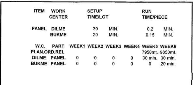
First of all the work centers for each production type must be defined in turn. The availability, utilization, efficiency for each work station must be known. The important two things are the "Setup Time per Lot" and "Run Time per Piece". Setup Time/Lot: It defines the setup time for the machinery, place, equipment, workers etc. All of the lot is processed after the setup. This setup time is not exactly considered in Rough Cut Capacity Planning.
Run Time/Piece: This is the time for producing one unit of item in one work center.
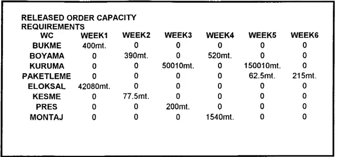
Capacity Requirements computation requires calculation of the setup time and run time separately. The setup time matrices are directly calculated from the planned order releases in MRP [Fogarty, 435]. When an order is released the standard setup time is written for that work station. Also the lead times make a shift for the next working station. The same calculation is done for the run time but the number of pieces are multiplied with the run time/piece. For each period the sum of each working station's capacity is taken. In order to have an exact calculation we
must take care of the capacity required by released orders. If there is a scheduled receipt for any product the setup and run time calculations must be done. Total sums of the three calculations give the capacity requirements of each work station for a given period.
2.7.3. Forward and Backward Scheduling
Forward and backward scheduling are the two terms frequently associated with the capacity requirements planning. In forward scheduling activities start at the planned released date and move forward in time. In backward scheduling, activities start at the planned receipt date and move backward in time.
If operation lead times add to the job lead time and operation time is assumed to occur at the end of the operation lead time, then forward scheduling and backward scheduling yield the same result. Some commercial and CRP systems use forward scheduling, others use backward scheduling. As long as the concepts are applied properly, the choice is not significant [Fogarty,439].
CHAPTER THREE
ANALYSIS
3.1. ABC AnalysisIn order to make an inventory management, materials must be classified. ABC analysis is done for the company called "Tacer" according to the annual dollar volume of the transactions. ABC classification is done considering years "1991,
1992, 1993".
3.1.1 Procedure for ABC Classification
First of all, daily sales records are organized and they are put into monthly sales. Unit cost of all items those are sold in July is converted to US dollars by dividing the prices to the number "30,800" ( 1$ is assumed to be 30800 TL in July) to have a constant unit price. It is assumed that the inflation rate in US dollar is negligible. The annual dollar sales of each item is found by multiplying the unit cost with the annual usage. The percentage effect of each item is found by dividing the annual dollar sales of each item to the total annual dollar sales. The items are listed from ascending to descending order and 20-30-50 percent criteria is accepted for classifying the class A-B-C items accordingly (see Table 1 of App.). The following results are obtained for each year according to the percentage in annual sales.
3.1.1.1. ABC Classes in 1991
Class A items:
• Panel • 1x40 Watt • Cita
They turned out to be the Class A items. 20 percent of the total items cost 77 percent of the total usage.
Class B items:
• Ikiz panel · U Profil
. Tas-U · Tel
• Yay
They turned out to be the Class B items. 30 percent of the total items cost 20 percent of the total usage.
Class C items: • 2x40Watt • Halojen • lx20Watt • Piton • Dübel 6 . Kulak • 2x20Watt • Vida 20x35
They turned out to be Class C items. 50 percent of the total items cost 3 percent of the total usage.
3.1.1.2 ABC Classes in 1992
In 1992: Class A items:
• Panel Cita
• lx40Watt · ikiz Panel
They turned out to be the Class A items. 20 percent of the total items cost 76 percent of the total usage.
Class B items:
• Kenar U · Ara Kayit • AnaTasiyici · lx20Watt
• Tavan C · Tas U
They turned out to be the Class B items. 30 percent of the total items cost 18 percent of the total usage.
Class C items: . L Profil • T sürgüsü . Kulak . Vida • Dubel 6 • Tavan U . Tel • Halojen • Yay . 20x35 • Piton
They turned out to be Class C items. 50 percent of the total items cost 6 percent of the total usage.
3.1.1.3. ABC Classes in 1993
In 1993: Class A items:
Panel • lx40Watt
Cita • ikiz Panel
Kenar U • Tasyunu
Tas U • Alcipan