On switching H ∞ controllers for a class of LPV systems

(1)

Proceedings of the 42nd IEEE

Conference on Decision and Control

Maui, Hawaii USA, December 2 W 3

FrPO1-4

On Switching H- Controllers for a Class of LPV Systems*

Peng

Yan

Dept.

of Electrical Engineering

The Ohio State

University

2015 Neil Ave. Columbus, OH 43210

yanp@ee.eng.ohio-state.edu

Abstracl- We consider switching 9P controllen for a class of LPV systems scheduled along a measurable parameter trajectory. The candidate controllen am selected from a given controller set according to the switching rules based on the scheduling variable. We provide sufficient conditions to guarantee the stability of the switching LPV systems in terms of the dwell time and the arerage dwell time. Our results are illustrated with an example, where switching between two robust controllen is performed for an LPV system.

I. INTRODUCTION

This paper addresses a switching H- control strategy for a class of linear parameter varying (LPV) systems scheduled along a measurable parameter trajectov. LPV systems are ubiquitous in chemical processes, robotics systems, automa- tive systems and many manufacturing processes. Meanwhile Jacobian linearization of nonlinear systems also results in LPV models, where gain scheduled controllers can be developed for the nonlinear plants. The analysis and control of LPV systems has been studied widely [l], [Z], [121, [17], [l8], [9], [161. A systematic gain scheduling method was developed in [l], [2] based on LMI (Linear Matrix Inequality) algorithms; [ 181 provided sufficient conditions for the stability of LPV systems with parameter-varying time delays, where gain scheduled controller was designed based on LMIs. Fast gain scheduling was considered in [9], where derivative information on the scheduling variable was utilized in a new control law. In a very recent publication [17], an improved stability analysis for LPV systems was given and the robust gain-scheduled controller was constructed in terms of LMIs. We refer to [13] for a general review on gain scheduling methods.

An alternative method is switching control where a family of controllers

are

designed at different operating points and the system performs controller switching based on the switching logic. As stated in [3], a challenging point of switching control is its hybrid nature of the continuous and discrete-valued signals. Stability analysis and the design methodology have been investigated recently in the literature of hybrid dynamical systems [61, 1111, [IO], [141, [15]. For LTI systems, I151 provided sufficient conditions on the stability of the switching control systems based on Filippov solutions to discontinuous differential equations and

*This work is supported in pan by AFOSR and A F R W A under

**Hilay Orbay is an lewe fmm The Ohio State University. agreement DO. F33615-01-2-3 154

Hitay Ozbay**

Dept.

of Electrical

&

Electronics Engineering

Bilkent University

Bilkent, Ankara, Turkey .TR-06800 ozbay@ee.eng.ohio-state.edu

Lyapunov functionals; [ll] proposed a dwell-time based switching control, where a sufficiently large dwell-time can guarantee the system stability. A more flexible result was obtained in [6], where the average dwell-time was introduced for switching control. Besides stability analysis, a number of results have been published on related topics, such as optimal control [14] and tracking problem [71.

Due to the time-varying and the hybrid natures of the switching LPV systems, it is challenging to explore the stability conditions and switching schemes similarly to those for LTI systems. Theoretical and practical results have been presented in recent publications [3], [lo], [13]. In particular, [3] analyzed the hounded amplitude performance and derived the conditions related to dwell time, and [lo] proposed switching H- controllers for nonlinear systems which ex- hibits LPV nature after linearization. In the present paper, we discuss the switching Hm control methodology for a class of LPV systems, where each candidate H- controller guarantees robust properly at the selected operating condition and the switching rules are developed to cover a large operating range. By constructing Lyapunov functionals for time-vwing systems as [41, [SI, this paper extends the stability results of [ti], [ I l l to LPV systems.

The paper is organized as follows. The problem definition is stated in Section 2, where the structure of the candidate H- controllers is described and the switching control ar- chitecture is proposed. In section 3, the

main

results on the stability of the switching systems are presented in terms of the dwell time and the average dwell time. An illustrative example is given in Section 4, followed by concluding remarks in Section 5.

11. PROBLEM

DEFINITION

The general structure of the switching control scheme that we consider in this paper is depicted in Figure 1, where w p E

Rn$$

is the exogenous input, U E R"" is the control input, z p E is the regulated output and y E

E%">

is the measured output. The LPV system depends on a parameter e ( t ) , where

O(r) E R is assumed to be continuously differentiable and 0 E 0 where 0 is a compact set.

Under further assumptions of

le(r)( < 6

and

le(r)l

<

p,

the stability and performance analysis of LPV system (1) can be formulated in terms of LMIs, where gain scheduling H- controllers can be derived based on convex optimization using LMIs [13], [l], [2], [121, [17]. In the present paper, we

(2)

Switching Logic

e

",,, wp ~ ~ ~ ~ y s t e m

*L

p(e)

Fig. 1. T h e switching control system

propose to construct a family of Ff- controllers designed at selected operating points

e

= Bi, i = I , 2, ....

I ,

and perform controller switching for the above LPV system, which allows for more freedom in the controller design and has the advantage of simplicity.

The candidate controllers are chosen from a controller set

4

:= { K ; ( s ) : i = 1,2, .... I } , where Ki(s) is an LTI Ff- controller designed at

e

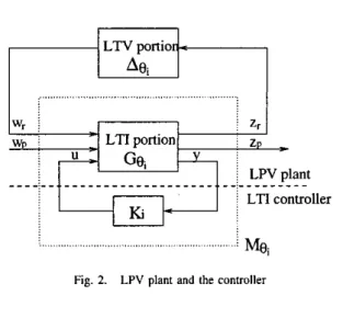
= 0;. Consider an operating range

Oi, Bi E O;, the LPV system in Figure 1 can he represented,

as F,(Ger,Ae;), where As, is the time varying portion of the LPV system, Get is the LTI portion with nominal value 0; and

Fu

denotes the upper LFT (Linear Fractional Transfor- mation). The closed loop system is depicted in Figure 2, where Gej is the nominal transfer function at a specified

e;:

and an Ff- optimization problem is defined as finding &(s)

for the LTI plant Ge, such that

(i). The closed loop system is asymptotically stable for 0 E 0..

(ii). inf{supWjo

#

: &(s)satisfies (i)}

5

y for the smallest possible y, where

I .

Denote

11.

Ilr.2 to he the Lz induced norm and let Me, to be the transfer function from

w,

to z,. A sufficient condition on robust stability satisfying (i) is []Me,

I/_

<

1 and IlAe, 111.2

<

1,

which can be obtained by applying small gain analysis [l],

[13], [19]. The above treatment results in the F P controller design for the LTI system, where standard

Ff-

optimization methods can be employed [ 5 ] . The state space expression of each candidate controller K , ( s ) is given by

Note that K;(s) robustly stabilizes the LPV system for

I/AejlJ;;2

<

1, which can be guaranteed by properly choosing

...

I !

w, i

; I

: 2,

i LTI controlle1 ...

:

Mei

Fig. 2. LPV plant and the controller

e,,

0: and

pi

>

0, such that

e

E

oi

:=

[e;,e:].

le(t)l

<pi.

(3) Accordingly, the robust bound Oi can be determined for each candidate controller Ki(s).

In order to cover a large operating range 0, we need to develop stable switching schemes over

4.

Obviously, a necessary condition for stable switching is:

0 d j O ; . (4)

i= I

111. MAIN RESULTS

Applying the switching rules over s a n d invoking (1) and (2). we obtain the closed loop A-matrix A,, E {Ai(e),i = 1,2> .... l } , where

A;(@) =

1

A

+

B ~ D K , ( I - & ~ D K ~ ) - ' C ~ &(I -DK,D~~)-'CK;

[

BK, ( I - DZZDK;)~'CZ AK, +BK;(I - DZZDK~)-'DZZCK; For switching LTI systems, it has been shown in [ l l ] that a sufficiently large dwell time can guarantee stability; and

[6] provided a more flexible and stronger result based on

the average dwell time. We claim that similar results can be obtained for switching LPV systems.

Consider the following switching LPV system:

= A q ( w 5 ( i ) , i 2 0 ( 5 ) where q is a piecewise constant signal taken values on the set

F

:= {1,2 ... l } , i.e. q ( t ) = i, i E f, for

Vr

E [t,,t,+l), where ij, j E ZfU{O}, is the j I h switching time instant. Here

A; E A := {A;(e(r)) : i E

F ,

e(r) E 0}, which is a family of parameter varying matrices. We further assume that: H I . There is a hi

>

0, such that for any 8 E 0, the eigen-

values of A i ( e ) have real parts no greater than -2hi,

V i €

F ;

(3)

H3. 3Kb

>

0,

1

1 v

1

1 5 Kb,

Vi E F ;

where

11. (1

denotes the (pointwise in time) Euclidean norm of a time-varying vector and the corresponding induced norm on matrices.

The dwell time based switching tule set is denoted by ~ [ T D ] , where TD is a constant such that for any q E s [ T D ] , the distance between any consecutive discontinuities of q ( f ) ,

lJ41 - f J , j E Z+U{O}, is larger than T D [6], [ill. Clearly

s[rDl]

c

s[rDZ], VTDl

>

TD2

>

0. (6)

A sufficient condition on the minimum dwell time to guarantee the stable switching can now he given using Lyapunov stability analysis (a similar result is obtained in [IO], using the same technique, for switched gain scheduling controllers in uncertain nonlinear systems).

77worem 3.1: Assume (Hl-H3). Then there exist finite constants

p

>

0, T D

>

0, such that the switching LPV system (5) is stable in the sense of Lyapunov for any switching d e q E S [ T D ] if le(t)l<

p.

Proof First we notice that

At(O(f)) :=A,(B(f))+h,I, V i €

f

(7)

is Hurwitz, which is straightforward fmm (Hl). Let

Note that Qi(r) is well defined, continuously differentiable, and is the unique positive-definite solution of

A?(e(t))Qi(f) +Qi(t)Ai(e(t)) = -1, (9) i.e.

Define a family of Lyapunov functions

7 , := {Vi :

K(t,t(f))

:= c T ( t ) Q i ( l ) c ( f ) , i E F } (11)

for the following LPV systems respectively

Note that differentiating (8) with respect to f gives Q i ( f ) = ~~p:(e(~i)i[aT(e(r))Qi(f)

+Qi(l)ai(e(f))]di(e(r))idi,

(15) (16)

a .

where

A;(e(f))

= s A i ( e ( t ) ) e ( f ) , I 2 0. Invoking (H3) and Lemma 3 of [8] we have

iiAi(e(r))lt

i

& e ( t ) i

IIQi(1)II

5 KhIe(f)I

(17) where Kh

>

0 is a constant depending only on hi, K i and

d.

_"

1

+

2hiMi P:=min{- Define i c ? K h Thus

Choosing the minimum dwell time as follows:

we claim that any switching rule q E S [ T D ] is stable in the (12) sense of Lyapunov.

((1) = A i ( e ( f ) ) l ( f ) , Vi E

F .

Consider an arbitrary switching interval [fj,tj+l), where

q ( t ) = i: i

E f,

for Vf E [ t j , l j + l ) . Using the quadratic form of Vi as shown in ( l l ) , a straightforward calculation gives the time derivative of Vi(t,<(t)) dong the trajectoty of (12)

(4)

stability of the overall switching system. Thus the proof is

complete. I

Pi = o m i u [ Q i ] , Mi = ~ u x [ Q i ] , V i E

F

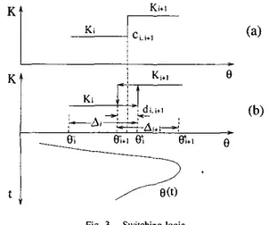
(24) where o,,zj,z[Qjl denotes the smallest singular value of Qj and onlox[Qj] the largest singular value of Qj.

The dwell time condition in Theorem 3.1 can be applied to the switching Ff- control problem discussed in Section 2. As depicted in Figure 3, two possible switching schemes [IO] are (a) critical-point switching, (h) hysteresis switching. For the critical-point switching, the stability of the closed- loop system cannot be guaranteed. In fact, in the worst case where O ( r ) oscillates within a neighborhood of cj.i+l, fast

switching or chattering will happen, which may violate the dwell time requirement. The following corollary addresses a sufficient condition for the hysteresis switching scheme over

H-

controller set

x.

Note that for switching LTI systems, we can set

t

Fig. 3. Swirching logic

Corollary 3.1: For the hysteresis switching over robust

controller set

i

with operating range 0; obeying (4), a sufficient condition to guarantee Lyapunov stability is

where &+I = Oin@+1 is the *'i hysteresis interval as shown in Figure 3.

Pmof: For simplicity, we consider only two neighboring controllers, i.e. Kj(s) and k ; + ~ ( s ) in switching time interval [ f j ; t j + l ) , j € Z+U{O}. As discussed in Theorem 3.1,

l j + i -. f j

>

TD should be satisfied to guarantee stability of the switching system, which requires the currently working controller K;(s) to hold on at least TD. In the worst case of switching where e ( t ) oscillates around the center of the interval & + I , with amplitude /d;,j+il/2, the condition

le(f)l

<

d j ; ; + l / T ~ is sufficient to guarantee stable switching. Taking all the possible controllers into consideration and

invoking (3) and

le(')/

<

0,

we come up with (25) and Note that Theorem 3.1, as well as Corollary 3.1, is in fact

conservative in the sense that the minimum dwell time should be satisfied, which does not allow for fast switching. In the following, we present another result based on the average dwell time for switching LPV systems, which can guarantee exponential stability of switching LPV systems in the more general sense.

Similar to [61, we define the average dwell time r;, and the corresponding switching rule set S,,,[r&.No] as follows. For f

>

5 2 0, let N ( f . T ) E Z+ U {0} denote the number of discontinuities (switching number) of a switching signal q in the time interval ( q r ) ; S.,.,[T&,N~] is defined as the set of all switching rules, q, that satisfy:

complete the proof.

where

bound. Obviously

is called the average dwell time and Nu the chatter

S[.r&]

c

&,.,[G,

11

In the rest of this section, a sufficient condition on the exponential stability is given in term of the average dwell time, which is an extension of theorem 1 of 161 to the switching LPV systems.

Theorem 3.2: Define

x

> 0 as bi rc!F

mi

h = pin{-}

where bi and Mi can he obtained from (20) and (13)

respectively. For Vh E

(O,h),

there exists T;

>

0 such that the switching LPV system ( 5 ) is exponentially stable with decay rate no slower than h for all the switching rules over

S o & , > N o ] , where No 2 0 is any finite chatter hound. Proof: Given time interval [IO,$ where i

>

Io = 0, denote

f l

< <

."

<

f N ( j , r 0 ) to he the switching time instants of q

in ( f O l i ) . Let

7

p := m a X { p } . le? Pi

Recall ( 2 2 ) , we have

-

(5)

For any h E

(O,x),

we define

where k

>

0 is a constant. Based on the definition of &,,,[7h,No], we come up with

i - t o N(l,to)

5

No

+

- 7; which is equivalent to - X ( l - r o ) +N(i.fo)lnp

5

k - h ( l - 10). ₍₃₃₎ Thus . . We conclude from (34) that the switching LPV system (5) is exponentially stable for all switching rules over S,,,[.rb,No]

with decay rate no slower than

A.

Recall (32). (27) and (281, we have

(35) Thus the average dwell time r; derived in Theorem 3.2 is larger than the minimum dwell time TD in Theorem 3.1. How- ever, the former doesn't require any minimum dwell time for switching, which could allow for some fast switchings.

Note that we assume e(r) is'a scalar function of time r in this paper. For the scenario e(t) E R"e being a vector, similar results can be easily obtained without funher complication.

IV. NUMERICAL EXAMPLE

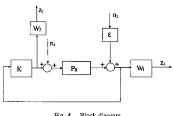
In this section, we apply the above switching H- control method to the following LPV system shown in Figure 4. We employ .L{f(rr8)Je=eo} = fe,(s) to describe the LPV dynamic equations in Laplace domain at fixed parameter values, by which the LPV plant Pe can be written as:

(36) where r = O . I , 00 = 10,

a =

15, So(@) =0.075e+0.085, and

O(r) =

e(r

+

7)

is periodical obeying (1

-

Ts)( 1 +as)

= (1

+

q ( s 2

+

25,,(e)wOS+ %)(I

-

as)

4ltr 3 3

T 8 8

8(r) = (3+2sin(-))(RJ(r)-RJ(r--T))+RJ(t--~)

where T = 3.6 x IO4 and W(r) is the unit step function. Thus

We would like to design 9Pcontrollers to stabilize the system and minimize sup,+o{&}, where the regulated output z and the exogenous input w are defined as:

0 E 0 := [1;5] and E,o(e) E [0.16,0.46].

Fig. 4. Block dia,qm

Note that n2 is a fictitious noise that we added so that the rank conditions of standard four block P design can be satisfied [5]. The weighting functions

Wl

and W2 are chosen as Wj = (s

+

100)/(4s

+

4) and Wz = 2 respectively.

We consider switching

P

control scheme as discussed in the above sections, where we design two 7P controllers K I and K2 at the selected operating points

e

= 81 = 2.2 and 8 = 82 = 3.8 respectively, and employ controller switching between K1 and K2. The operating range is chosen as 01 =

[e;,e:]

= [1,3.4] for controller KI, and 0 2 =

[ei,e;]

= [2.6,5] for K2. The two candidate 9P controllers Kj and K2

can be constructed using standard 9P optimization methods [SI,

[W:

9654s4

+

1.54 x IO5$

+

1.59 x 106s2

+

1 . 1 I x 107s+9.64 x IO6 9

+

8 8 . 4 8 ~ ~

+

1 7 1 0 ~ ~

+

2.93 x 104s2 +2.96 x IO4,+ 1840 and

[

*

I

-

K2 =

9661s4+1.78 x 1OSs3+1.85 x IO6?+ 1.13 x IO'st9.64~ IO6 s"+89.83s4+1815sS+3.04x 10"s2+3.05x 104s+1901 The following analysis shows that K1 and K2 can robustly stabilize the LPV system within the operating range 01 and

0 2 respectively.

Define

P ; ( s ) = P e ( s ) - P e j ( s ) , i = 1,2, and assume

I ~ L ( j o ) l

<

IWjl,i= 1,2. (37)

A sufficient condition to guarantee robust stability is given by [19]:

(38)

llw&(l+~e~~;)-'II-

5 1, i = 1,2.

As depicted in Figure 5 , (37) can be satisfied by choosing 55(s+2)* (s

+

7)2(s

+

S)(s + 9 ) ( s

+

12) 30(s

+

2)2 (s

+

7 ) 2 ( s + S)(s +9)(r

+

12) W,(s) = W,'(.Y) =

(6)

. . . . . . . _{. . .} . . . . . . . . . . . . 30-J ' ' ' ' 10-3 1 0" 70- 1 0' IreqYBnCY ~radlseC)

Fi:. 5. Weights for unceminties with respect to 91 and 82

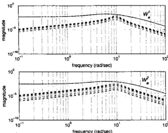
Figure 6 shows that the robust stability condition (38) is satisfied for

K I

and

Kz

respectively.

frequency (radhac)

Fig. 6. Robustness test

Thus

K,

and K2 can robustly stabilize the LPV system with respect to 01 and 02. Consider the closed-loop A-matrices

A 1 ( 6 ) , e E 01 and A2(0),6 E 02. we can numerically obtain the following parameters:

TABLE I

P A R A M ~ T E R s X , , ~ , . M , A N D K ~

.

i = l 0.8 1.0 261.59 3028.2 i = ? 261.49 1190.9

Recall (IS), we have

p

= 8.6 x Also notice that 41f

18000 le(t)l

I

1-1

=

7~

Choosing

p

= 8.1 x

<

p

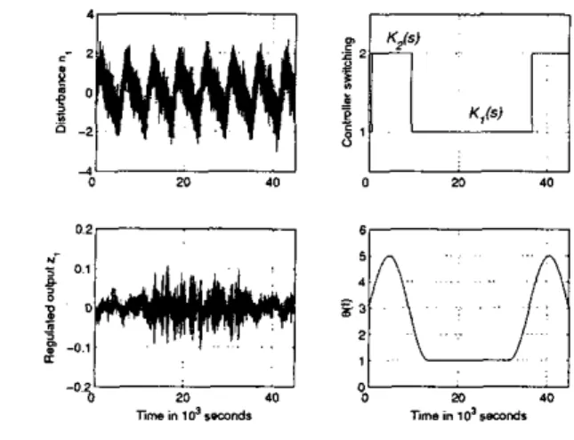
and invoking (20), we have

bl = 0.15 and b2 = 2.84. Furthermore, we can pick h = 1.02 x such that T; = 1.5 x lo4, which is straightforward from (27), (28) and (32). Thus, the switching scheme for e(t) belongs to Sa,,&, I], which is due to the fact that there are only 2 switcbings per period T (Fig.8). Based on Theorem 3.2, we conclude that the switching LPV system with

K I

ind K2 are stable.

The closed loop system with the determined switching H- control scheme is simulated using MATLAB. For the purpose of comparison, we also provide an H- controller

i?

designed at 6 =

9

= 3 for the LPV system, by which the performance of a single H- controller can be simulated. The disturbance n1 is set to be n l ( t ) = sin(21f/6000)

+

1

sin(2n/3000)

+

S(t), where S(t) is a Gaussian distributed signal of mean 0 and variance 0.2.

e-+e+ . . . .

-

5 I I Time in lo3 w m d s

8

3 1 0 1 5 2 0 2 5 3 0 3 5 U I 1 3

Fig. 7. The case of a single 9 P conmllei

First, we give the simulation result for tbe case of single H- controller

i?

(for comparison purposes) in Figure 7,

where the divergence of the output signal is observed because

i?

itself can not robustly stabilize the LPV system for the whole operating range 0. The simulation results of the switching H- control method are depicted in Figure 8. Note that the system remains stable and the magnitude of the regulated output zl is much smaller than the magnitude of the disturbance nl for all 6 E 0.

Note that for the proposed switching control scheme, Theorem 3.1 is not valid. In fact, the minimum dwell time

TD to guarantee stability in Theorem 3.1 is given by 2 ~ i In

i=1.2 b;

TD = m a { } = 9.71 x 10'

>

T,,,;,,,

where ~~j~ = T/4 = 9000 is the minimum distance between

two consecutive switchings in our design, which is depicted in Fig.8. Meanwhile, Corollary 3.1 also turns out to be too

(7)

Fig. 8. The switching 3l“cantrol methcd

conservative for this design due to the fact that

which violates (25). The analysis of this numerical example affirms a good coincidence with the discussion of Section 3. It suggests that Theorem 3.2 is a less conservative result allowing faster switching.

V. CONCLUDING REMARKS

Switching 9P controllers are proposed for a class of LPV systems with slow parameter variations. Controller robustness is combined with the switching policy, which results in the hysteresis switching over a set of H-= controllers designed at selected operating points. The stability analysis is provided in terms of the dwell time and the average dwell time. The proposed switching 7P control method is

illustrated by a numerical example, where the comparison between the single 9P conmller and our design is also given. A further extension of this work would be switching control for LPV systems with fast parameter variations.

VI. REFERENCES

[ 1

J

P. Apkarian and P. Gahinet, ‘A convex characterization of gain-scheduled H- controllers”, IEEE Trans. Auto-

nuzric Control, vol. 40, pp. 853-864, 1995.

P. Apkarian, P. Gahinet and G. Becker, “ Self-scheduled H- control of linear parameter-varying systems: a design example”, Automatica, vol. 31, pp. 1251-1261, 1995.

C. Belt and M. Lemmon, “Bounded amplitude performance of switched LPV systems with applications to hybrid systems”, Autonuztica, vol. 35, pp. 491-503, 1999.

C. Desoer, “Slowly varying system i = A(t)x”, IEEE Trans. Automatic Control, vol. 14, pp. 780-781, 1969.

151 J. Doyle, K. Glover, P. Khargonekar and

B.

Francis, “State-space solutions to standard H2 and control problems”, IEEE Trans. Autonlotic Control, vol. 34, pp. 831-847, 1989.

[6] J. Hespanha and S. Morse, “Stability of switched sys- tems with average dwell-time”, Pmc. of the 38th IEEE

Conference on Decision and Control, 1999.

[71 J. Hochcerman-Frommer, S. Kulkarni and P. Ramadge, “Controller switching based on output prediction er- rors”, IEEE Trans. Autonutic Control. vol. 43, pp. 596- 607, 1998.

[SI D. Lawrence and W. Rugh, “On a stability theorem for nonlinear systems with slowly varying inputs”, IEEE Trans. Autonuzric Control, vol. 35, pp. 860-864, 1990. [9] S.-H. Lee and J.-T. Lim, “Fast gain scheduling on tracking problems using derivative information”, Auto- matica, vol. 33, pp. 2265-2268, 1997.

[lo] S.-H. Lee and J.T. Lim, “Switching control of 9f- gain scheduled controllers in uncertain nonlinear systems”,

Autoniatica, vol. 36, pp. 1067-1074, 2000.

[I I] S. Morse, “Supervisory control of families of linear set- point controllers: part 1: exact matching”, IEEE Trans. Automatic Control, vol. 41, pp. 1413-1431, 1996. [I21 A. Packard, “Gain-scheduling via linear fractional trans-

formations”, System and Control Lerrer.s, vol. 22, pp. 79-92, 1994.

[I31 W. Rugh and J. Shamma, “Research on gain schedul- ing”, Automatica, vol. 36, pp. 1401-1425, 2000. [14] A. Savkin, E. Sakfidas and R. Evans, “Robust output

feedback stabilizability via controller switching”, Sys-

tem and Control Letters, vol. 29, pp. 81-90, 1996. [15] E. Skalidas, R. Evans, A. Savkin and I. Peterson,

“Stability results for switched controller systems”, Au-

tomatica, vol. 35, pp. 553-564, 1999.

[16] D. Stilwell and W. Rugh, “Stability and

Lz

gain prop- erties of LPV systems”, Pmc. of the American Contml Conference, 1999.

[I71 F. Wang and

V.

Balakrishnan, “Improved stability analysis and gain-scheduled controller synthesis for parameter-dependent systems”, IEEE Trans. Automatic Control, vol. 47, pp. 720-734, 2002.

[18]

E Wu

and

K.

Grigoriadis, “LPV systems with parameter-varying time delays: analysis and control”,

Automatica, vol. 37, pp. 221-229, 2001.

[I91 K. Zhou, J. Doyle and K. Glover, “Robust and Optimal Control”, Prenrice-Hall, New Jersey, 1996.