Radius of curvature estimation and localization of targets using multiple sonar sensors

Radius of curvature estimation and localization of targets using multiple sonar sensors

Billur Barshan, and Ali Şafak Sekmen

Citation: The Journal of the Acoustical Society of America 105, 2318 (1999); doi: 10.1121/1.426838 View online: http://dx.doi.org/10.1121/1.426838

View Table of Contents: http://asa.scitation.org/toc/jas/105/4

Radius of curvature estimation and localization of targets

using multiple sonar sensors

Billur Barshan

Department of Electrical Engineering, Bilkent University, Bilkent, 06533 Ankara, Turkey

Ali S¸ afak Sekmen

Center for Intelligent Systems, Department of Electrical and Computer Engineering, Vanderbilt University, Box 1824, Station B, Nashville, Tennessee 37235

~Received 12 August 1998; accepted 31 December 1998!

Acoustic sensors have been widely used in time-of-flight ranging systems since they are inexpensive and convenient to use. One of the most important limitations of these sensors is their low angular resolution. To improve the angular resolution and the accuracy, a novel, flexible, and adaptive three-dimensional ~3-D! multi-sensor sonar system is described for estimating the radius of curvature and location of cylindrical and spherical targets. Point, line, and planar targets are included as limiting cases which are important for the characterization of typical environments. Sensitivity analysis of the curvature estimate with respect to measurement errors and certain system parameters is provided. The analysis and the simulations are verified by experiments in 2-D with specularly reflecting cylindrical and planar targets, using a real sonar system. Typical accuracies in range and azimuth are 0.18 mm and 0.1°, respectively. Accuracy of the curvature estimation depends on the target type and system parameters such as transducer separation and operating range. The adaptive configuration brings an improvement varying between 35% and 45% in the accuracy of the curvature estimate. The presented results are useful for target differentiation and tracking applications. © 1999 Acoustical Society of America.@S0001-4966~99!03904-1#

PACS numbers: 43.58.2e, 43.28.Tc, 43.60.Qv, 43.35.Yb @SLE#

INTRODUCTION

Ultrasonic transducers are a convenient and inexpensive means for intelligent systems to build models of their envi-ronment. However, these sensors are limited by their wide beamwidth which makes accurate localization of targets dif-ficult. To increase the localization accuracy, an adaptive sen-sor configuration composed of multiple ultrasonic transduc-ers is proposed that is capable of estimating the radius of curvature and location of spheres, cylinders, point, line, and planar targets. Consequently, these basic types of reflectors can be differentiated.

Target localization has been extensively studied in ear-lier work. In Ref. 1, time-delay estimation for active/passive localization in underwater sonar is reviewed with references to benchmark work. In particular, ocean effects which re-quire sonar adaptation are considered. Adaptive sonar arrays have been also used by other researchers to add flexibility to their systems.2 Coherent and incoherent processing tech-niques of time-delay estimation have been addressed in Refs. 3, 4. Active, wide-band detection and localization of targets in a dense and uncertain multipath environment has been considered in Ref. 5. The review article in Ref. 6 considers numerical schemes for accurate processing of information from both active and passive acoustic arrays.

Sonar sensing has many applications for intelligent sys-tems operating in three-dimensional ~3-D! environments, such as airborne or underwater robots. Several researchers have investigated the limitations of sonar for 3-D target rec-ognition, discrimination, and tracking: Self-contained navi-gation systems have been devised for underwater vehicles,

capable of tracking and producing continuous range informa-tion from a passive target.7 In Ref. 8, an approach is de-scribed to the construction of 3-D stochastic models for in-telligent systems exploring the underwater environment. In Ref. 9, the minimum amount of information and actuation needed to track a ball in 3-D has been determined and imple-mented using qualitative methods. Hong and Kleeman have investigated the geometry of 3-D corner cubes using a low-sample rate equilateral triangular sonar configuration.10 Kleeman and Akbarally have classified and discriminated the target primitives commonly occurring in 3-D space.11 Pere-mans et al.12and Sabatini13,14both have investigated curved reflectors using linear array configurations. In Ref. 15, an analytical approach to surface curvature extraction is de-scribed which employs ultrasonic echo trajectories and dif-ferential geometry. In Refs. 16 and 17, binaural sonar infor-mation is fused for accurate object recognition using a system which adaptively changes its position and configura-tion in response to the echoes it detects. Curvature estimaconfigura-tion has been also important in image analysis to provide viewpoint-independent cues for shape classification.18

Some sonar systems attempt to emulate the remarkable perception and pattern recognition capabilities of bats and dolphins in extracting detailed information about their envi-ronments from acoustic echo returns.19–21 Artificial neural networks have been widely used for this purpose, to process time and/or frequency representations of sonar echo signals. For example, one application is in the classification of sonar returns from undersea targets where the targets may be made of different materials, have different shape, buried in mud or sediment, or exist in the presence of other reflectors in the

environment.21–23In Ref. 24, cylinder-wall thicknesses dis-criminating capability of artificial neural networks is com-pared to that of dolphins. In Ref. 25, artificial neural net-works are applied to classifying underwater active sonar returns with different numbers of peaks. Another system can recognize 3-D cubes and tetrahedrons, independent of their orientation with the help of neural networks.19

Acoustic imaging of extended targets by means of synthetic-aperture sonar has been considered in Ref. 26, where echoes from spherical and cylindrical targets laid down on a seabed are processed together with random ech-oes from the sea bottom. In Ref. 27, Stergiopoulos reviews the implementation of adaptive synthetic-aperture processing schemes in integrated active–passive sonar systems.

In this paper, an adaptive sonar configuration is used for radius of curvature estimation and localization of targets. When the reflection point of the target is not along the line-of-sight of the transducer, the amplitude of the reflected sig-nal is smaller, which decreases the sigsig-nal-to-noise ratio

~SNR! and worsens the accuracy. To reduce this effect, the

transducers are rotated toward the target to obtain more nearly accurate estimates.

The organization of the paper is as follows: In Sec. I, background information on acoustic reflection and signal models of sonar sensors is reviewed and motivation for the adaptive configuration is provided. Methods for time-of-flight estimation are discussed in Sec. II. In Sec. III, the geometry of reflection from spherical targets is considered and analyzed for radius of curvature estimation. The impor-tant limiting cases of point and planar targets are highlighted. Sensitivity analysis of curvature estimation is provided with respect to measurement errors and variations in some of the system parameters in Sec. IV. Section V presents the simu-lation results. A detailed description of the sensing device used in this study is provided in Sec. VI A. Experimental results which verify the analysis and the simulations are pre-sented in Sec. VI B. Section VII briefly discusses the use of the method for target differentiation. Finally, conclusions are drawn and directions for future work are motivated.

I. ACOUSTIC REFLECTION AND SIGNAL MODELS

The characteristics of the radiation pattern of an acoustic transducer are different in the near-field ~or Fresnel! region and the far-field ~or Fraunhofer! region.28 In this study, as-suming all targets of interest are located in the far field, the far-field model of a piston-type transducer having a circular aperture is used.28 For a single frequency of excitation, the far-field characteristics at range z and angular deviation a from the line-of-sight are described by29,30

pz,a5

pmaxzmin

z

J1~ka sina!

ka sina for z>zmin, ~1!

where J1(.) is the Bessel function of the first order of the first kind and pmaxis the propagation pressure amplitude on the beam axis at range zmin along the line-of-sight. zmin

>a2_{/l is the distance at which the far-zone characteristics} begin. Although the 2-D cross-section of the characteristics

is given here, in fact, the pattern is rotationally symmetric about the line-of-sight.

The half beamwidth angle a0 in the far-field corre-sponds to the first zero of the Bessel function in Eq. ~1! which occurs at ka sina051.22p, resulting in:31

a05sin21

F

a

G

where l5c/ f0 is the wavelength ( f0 is the resonance fre-quency of the transducer! and a is the transducer aperture radius.

Since a range of frequencies around f0 are transmitted, the corresponding beam patterns are superposed and the re-sulting pattern can be approximated by a Gaussian function centered at zero with standard deviation s_a5a0/2:

32 p ˜_z,a5pmaxzmin z e 2a2_/2s a 2 for z>zmin. ~3!

For a rigid cylindrical target of infinite height at range z and making an angle a with the line-of-sight of the trans-ducer, the received time signal can be modeled by:33

s_z,a~t!5r_cAmaxzmin 3/2 z3/2 e 2a2_/s a 2 e2 [t2~t01Dtc!]2/2st 2

3sin@2pf0~t2t0!# for z>zmin, ~4! where r_c is the reflection coefficient which increases with the radius of curvature,34Amaxis the maximum signal ampli-tude, z is the distance between the transducer and the object surface, t0 is the time-of-flight, Dtc is the time difference between the center of the Gaussian window and t0, and st 51/f0. Basically, the received signal envelope has been modeled as a Gaussian function centered at t01Dtc with suitably chosen variances_t2.33 More generally, the model

sz,a~t!5k~z!e2a 2_/s a 2 e2 [t2~t01Dtc!]2/2st 2

3sin@2pf0~t2t0!# for z>zmin ~5! is capable of representing observed signals for a wide variety of target types and locations in the far zone.33 Here, k(z) incorporates Amax and rc, and is inversely proportional to some power of the range z depending on target type.35 The inclination angle a from the line-of-sight is related to the target azimuth and elevation angles u andf by the relation

a5cos21_(cosucosf).

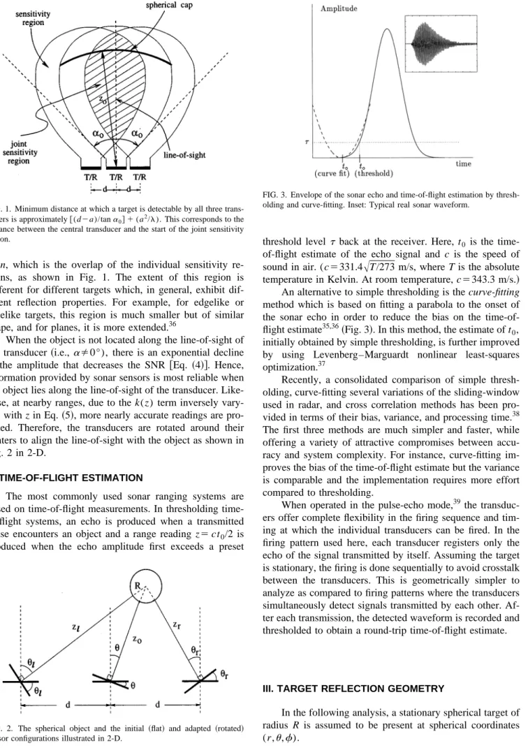
With a single stationary transducer, it is not possible to estimate the angular position of the target (u,f) with better resolution than the angular resolution of the transducer which is approximately 2a₀. When a range reading is re-ceived, all that is known is that the object lies somewhere on a spherical cap subtending a cone of half anglea₀ and radius

z, centered at the transducer. This is illustrated in Fig. 1 in

2-D for the transducer in the middle. To improve the angular resolution, the present system employs multiple identical acoustic transducers with center-to-center separation d ~Fig. 1!. Each transducer can operate both as transmitter and as receiver and detect echo signals reflected from targets within its sensitivity region. All members of the sensor configura-tion can detect targets located within the joint sensitivity

gion, which is the overlap of the individual sensitivity

re-gions, as shown in Fig. 1. The extent of this region is different for different targets which, in general, exhibit dif-ferent reflection properties. For example, for edgelike or polelike targets, this region is much smaller but of similar shape, and for planes, it is more extended.36

When the object is not located along the line-of-sight of the transducer ~i.e.,aÞ0°), there is an exponential decline in the amplitude that decreases the SNR @Eq. ~4!#. Hence, information provided by sonar sensors is most reliable when the object lies along the line-of-sight of the transducer. Like-wise, at nearby ranges, due to the k(z) term inversely vary-ing with z in Eq.~5!, more nearly accurate readings are pro-vided. Therefore, the transducers are rotated around their centers to align the line-of-sight with the object as shown in Fig. 2 in 2-D.

II. TIME-OF-FLIGHT ESTIMATION

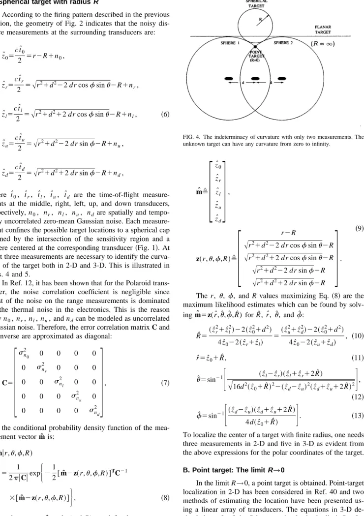
The most commonly used sonar ranging systems are based on of-flight measurements. In thresholding time-of-flight systems, an echo is produced when a transmitted pulse encounters an object and a range reading z5 ct0/2 is produced when the echo amplitude first exceeds a preset

threshold level t back at the receiver. Here, t0 is the time-of-flight estimate of the echo signal and c is the speed of sound in air. (c5331.4

A

temperature in Kelvin. At room temperature, c5343.3 m/s.! An alternative to simple thresholding is the curve-fitting method which is based on fitting a parabola to the onset of the sonar echo in order to reduce the bias on the time-of-flight estimate35,36~Fig. 3!. In this method, the estimate of t₀, initially obtained by simple thresholding, is further improved by using Levenberg–Marguardt nonlinear least-squares optimization.37

Recently, a consolidated comparison of simple thresh-olding, curve-fitting several variations of the sliding-window used in radar, and cross correlation methods has been pro-vided in terms of their bias, variance, and processing time.38 The first three methods are much simpler and faster, while offering a variety of attractive compromises between accu-racy and system complexity. For instance, curve-fitting im-proves the bias of the time-of-flight estimate but the variance is comparable and the implementation requires more effort compared to thresholding.

When operated in the pulse-echo mode,39 the transduc-ers offer complete flexibility in the firing sequence and tim-ing at which the individual transducers can be fired. In the firing pattern used here, each transducer registers only the echo of the signal transmitted by itself. Assuming the target is stationary, the firing is done sequentially to avoid crosstalk between the transducers. This is geometrically simpler to analyze as compared to firing patterns where the transducers simultaneously detect signals transmitted by each other. Af-ter each transmission, the detected waveform is recorded and thresholded to obtain a round-trip time-of-flight estimate.

III. TARGET REFLECTION GEOMETRY

In the following analysis, a stationary spherical target of radius R is assumed to be present at spherical coordinates (r,u,f).

FIG. 1. Minimum distance at which a target is detectable by all three trans-ducers is approximately@(d2a)/tana0# 1 (a2/l). This corresponds to the

distance between the central transducer and the start of the joint sensitivity region.

FIG. 2. The spherical object and the initial ~flat! and adapted ~rotated! sensor configurations illustrated in 2-D.

FIG. 3. Envelope of the sonar echo and time-of-flight estimation by thresh-olding and curve-fitting. Inset: Typical real sonar waveform.

A. Spherical target with radiusR

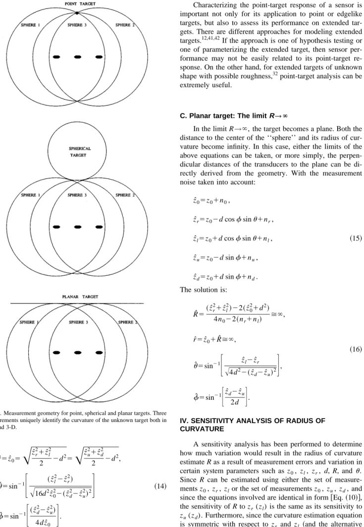
According to the firing pattern described in the previous section, the geometry of Fig. 2 indicates that the noisy dis-tance measurements at the surrounding transducers are:

zˆ05 c tˆ0 2 5r2R1n0, zˆr5 c tˆr 2 5

A

A

A

A

where tˆ₀, tˆ_r, tˆ_l, tˆ_u, tˆ_d are the time-of-flight measure-ments at the middle, right, left, up, and down transducers, respectively, n₀, n_r, n_l, n_u, n_d are spatially and tempo-rally uncorrelated zero-mean Gaussian noise. Each measure-ment confines the possible target locations to a spherical cap defined by the intersection of the sensitivity region and a sphere centered at the corresponding transducer~Fig. 1!. At least three measurements are necessary to identify the curva-ture of the target both in 2-D and 3-D. This is illustrated in Figs. 4 and 5.

In Ref. 12, it has been shown that for the Polaroid trans-ducer, the noise correlation coefficient is negligible since most of the noise on the range measurements is dominated by the thermal noise in the electronics. This is the reason why n0, nr, nl, nu, and ndcan be modeled as uncorrelated Gaussian noise. Therefore, the error correlation matrix C and its inverse are approximated as diagonal:

C5

3

4

and the conditional probability density function of the mea-surement vector mˆ is:

p~mˆur,u,f,R! 5 1 2puCuexp

H

J

mˆ,

F

G

F

A

A

A

A

G

The r, u, f, and R values maximizing Eq. ~8! are the maximum likelihood estimates which can be found by solv-ing mˆ5z(rˆ,uˆ ,fˆ ,Rˆ) for Rˆ, rˆ,uˆ , andfˆ :

Rˆ5~zˆr 2_1zˆ l 2_!22~zˆ 0 2_1d2_! 4zˆ022~zˆr1zˆl! 5~zˆu 2_1zˆ d 2_!22~zˆ 0 2_1d2_! 4zˆ022~zˆu1zˆd! , ~10! rˆ5zˆ01Rˆ, ~11! uˆ_5sin21

F

A

G

F

G

To localize the center of a target with finite radius, one needs three measurements in 2-D and five in 3-D as evident from the above expressions for the polar coordinates of the target.

B. Point target: The limit R_˜0

In the limit R→0, a point target is obtained. Point-target localization in 2-D has been considered in Ref. 40 and two methods of estimating the location have been presented us-ing a linear array of transducers. The equations in 3-D de-rived above for finite R become simpler in the limit R→0:

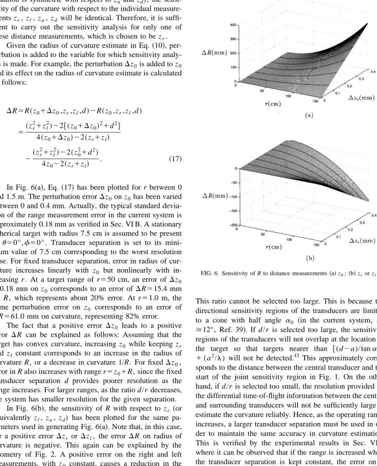
FIG. 4. The indeterminacy of curvature with only two measurements. The unknown target can have any curvature from zero to infinity.

rˆ5zˆ₀5

A

A

F

A

G

F

G

Characterizing the point-target response of a sensor is important not only for its application to point or edgelike targets, but also to assess its performance on extended tar-gets. There are different approaches for modeling extended targets.12,41,42If the approach is one of hypothesis testing or one of parameterizing the extended target, then sensor per-formance may not be easily related to its point-target re-sponse. On the other hand, for extended targets of unknown shape with possible roughness,32point-target analysis can be extremely useful.

C. Planar target: The limit R_˜`

In the limit R→`, the target becomes a plane. Both the distance to the center of the ‘‘sphere’’ and its radius of cur-vature become infinity. In this case, either the limits of the above equations can be taken, or more simply, the perpen-dicular distances of the transducers to the plane can be di-rectly derived from the geometry. With the measurement noise taken into account:

zˆ₀5z₀1n₀,

zˆr5z02d cosfsinu1nr,

zˆ_l5z₀1d cosfsinu1n_l, ~15!

zˆu5z02d sinf1nu, zˆd5z01d sinf1nd. The solution is:

Rˆ5~zˆr 2_1zˆ l 2_!22~zˆ 0 2_1d2_! 4n₀22~n_r1n_l! >`, rˆ5zˆ01Rˆ>`, ~16! uˆ_5sin21

F

A

G

F

G

IV. SENSITIVITY ANALYSIS OF RADIUS OF CURVATURE

A sensitivity analysis has been performed to determine how much variation would result in the radius of curvature estimate R as a result of measurement errors and variation in certain system parameters such as z0, zl, zr, d, R, and u. Since R can be estimated using either the set of measure-ments z0, zr, zlor the set of measurements z0, zu, zd, and since the equations involved are identical in form@Eq. ~10!#, the sensitivity of R to zr (zl) is the same as its sensitivity to zu(zd). Furthermore, since the curvature estimation equation is symmetric with respect to zr and zl ~and the alternative FIG. 5. Measurement geometry for point, spherical and planar targets. Three

measurements uniquely identify the curvature of the unknown target both in 2-D and 3-D.

equation is symmetric with respect to zu and zd), the sensi-tivity of the curvature with respect to the individual measure-ments zr, zl, zu, zd will be identical. Therefore, it is suffi-cient to carry out the sensitivity analysis for only one of these distance measurements, which is chosen to be zr.

Given the radius of curvature estimate in Eq. ~10!, per-turbation is added to the variable for which sensitivity analy-sis is made. For example, the perturbationDz0is added to z0 and its effect on the radius of curvature estimate is calculated as follows: DR5R~z01Dz0,zr,zl,d!2R~z0,zr,zl,d! 5~zr 2_1z l 2_!22@~z 01Dz0!21d2# 4~z01Dz0!22~zr1zl! 2~zr 2_1z l 2_!22~z 0 2_1d2_! 4z₀22~z_r1z_l! . ~17!

In Fig. 6~a!, Eq. ~17! has been plotted for r between 0 and 1.5 m. The perturbation errorDz0on z0 has been varied between 0 and 0.4 mm. Actually, the typical standard devia-tion of the range measurement error in the current system is approximately 0.18 mm as verified in Sec. VI B. A stationary spherical target with radius 7.5 cm is assumed to be present at u50°,f50°. Transducer separation is set to its mini-mum value of 7.5 cm corresponding to the worst resolution case. For fixed transducer separation, error in radius of cur-vature increases linearly with z0 but nonlinearly with in-creasing r. At a target range of r550 cm, an error of Dz0

50.18 mm on z0 corresponds to an error ofDR515.4 mm on R, which represents about 20% error. At r51.0 m, the same perturbation error on z0 corresponds to an error of

DR561.0 mm on curvature, representing 82% error.

The fact that a positive error Dz0 leads to a positive error DR can be explained as follows: Assuming that the target has convex curvature, increasing z0 while keeping zr and zl constant corresponds to an increase in the radius of curvature R, or a decrease in curvature 1/R. For fixedDz0, error in R also increases with range r5z01R, since the fixed transducer separation d provides poorer resolution as the range increases. For larger ranges, as the ratio d/r decreases, the system has smaller resolution for the given separation.

In Fig. 6~b!, the sensitivity of R with respect to zr ~or equivalently zl, zu, zd) has been plotted for the same pa-rameters used in generating Fig. 6~a!. Note that, in this case, for a positive error Dz_r or Dz_l, the error DR on radius of curvature is negative. This again can be explained by the geometry of Fig. 2. A positive error on the right and left measurements, with z₀ constant, causes a reduction in the radius of curvature.

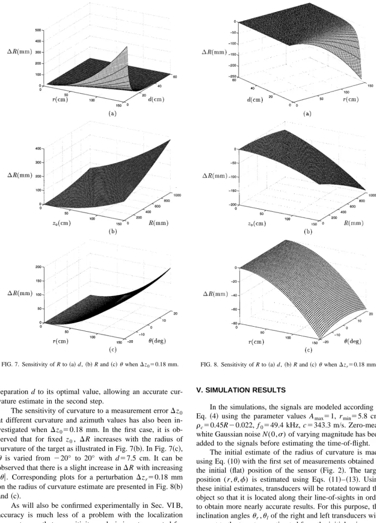
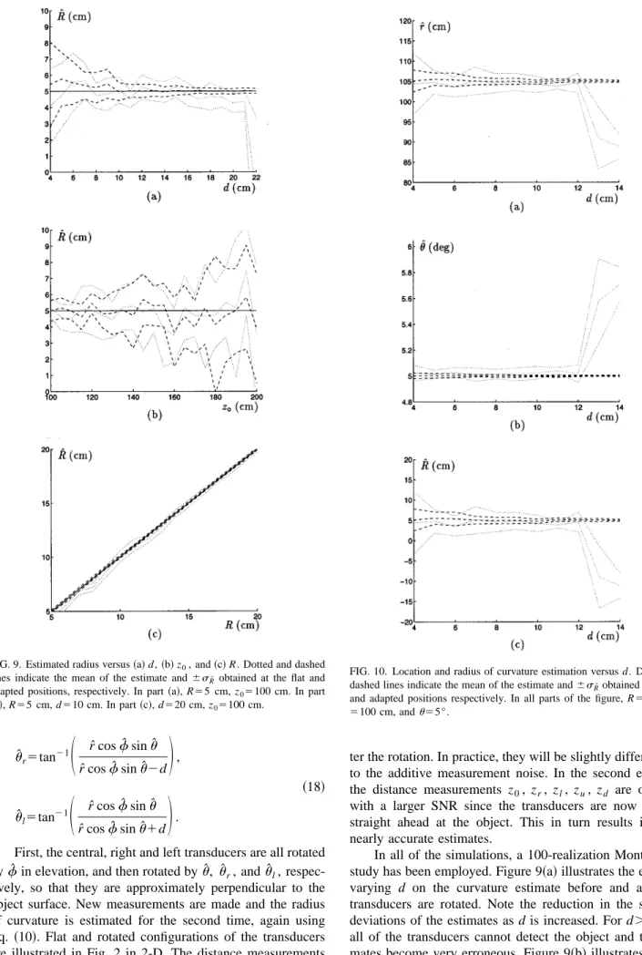
Fig. 7~a! illustrates the effect of transducer separation d on the accuracy of the radius of curvature estimate. For r between 0 and 1.5 m andDz050.18 mm, Eq. ~17! has been plotted for transducer separations between 4.0 and 60 cm. Corresponding plot for Dzr50.18 mm is presented in Fig. 8~a!. In both figures, it is observed that the ratio d/r is a significant parameter in the curvature estimation process.

This ratio cannot be selected too large. This is because the directional sensitivity regions of the transducers are limited to a cone with half angle a0 ~in the current system, a0

>12°, Ref. 39!. If d/r is selected too large, the sensitivity

regions of the transducers will not overlap at the location of the target so that targets nearer than @(d2a)/tana0#

1 (a2_{/l) will not be detected.}43 _{This approximately} corre-sponds to the distance between the central transducer and the start of the joint sensitivity region in Fig. 1. On the other hand, if d/r is selected too small, the resolution provided by the differential time-of-flight information between the central and surrounding transducers will not be sufficiently large to estimate the curvature reliably. Hence, as the operating range increases, a larger transducer separation must be used in or-der to maintain the same accuracy in curvature estimation. This is verified by the experimental results in Sec. VI B where it can be observed that if the range is increased while the transducer separation is kept constant, the error on R increases. Thus, it is concluded that a sensor system which is to operate over a large range of target distances must have the capability of adaptively adjusting transducer separation

d. The information provided by Figs. 1 and 6~a! can be

com-bined to formulate a rule for choosing the optimal transducer separation d for a given range r. Thus, one can envisage a two-step curvature estimation process: The range estimate obtained in the first step is used to adjust the transducer

separation d to its optimal value, allowing an accurate cur-vature estimate in the second step.

The sensitivity of curvature to a measurement errorDz0 at different curvature and azimuth values has also been in-vestigated when Dz₀50.18 mm. In the first case, it is ob-served that for fixed z₀, DR increases with the radius of curvature of the target as illustrated in Fig. 7~b!. In Fig. 7~c!,

u is varied from 220° to 20° with d57.5 cm. It can be observed that there is a slight increase inDR with increasing

uuu. Corresponding plots for a perturbation Dzr50.18 mm on the radius of curvature estimate are presented in Fig. 8~b! and~c!.

As will also be confirmed experimentally in Sec. VI B, accuracy is much less of a problem with the localization parameters so that a sensitivity analysis is not presented for these parameters.

V. SIMULATION RESULTS

In the simulations, the signals are modeled according to Eq. ~4! using the parameter values Amax51, rmin55.8 cm,

rc50.45R20.022, f0549.4 kHz, c5343.3 m/s. Zero-mean white Gaussian noise N(0,s) of varying magnitude has been added to the signals before estimating the time-of-flight.

The initial estimate of the radius of curvature is made using Eq.~10! with the first set of measurements obtained at the initial ~flat! position of the sensor ~Fig. 2!. The target position (r,u,f) is estimated using Eqs. ~11!–~13!. Using these initial estimates, transducers will be rotated toward the object so that it is located along their line-of-sights in order to obtain more nearly accurate results. For this purpose, the inclination anglesur,ulof the right and left transducers with respect to the target are estimated from the initial noisy mea-surements:

uˆ_r5tan21

S

D

S

D

First, the central, right and left transducers are all rotated byfˆ in elevation, and then rotated byuˆ , uˆ_r, anduˆ_l, respec-tively, so that they are approximately perpendicular to the object surface. New measurements are made and the radius of curvature is estimated for the second time, again using Eq. ~10!. Flat and rotated configurations of the transducers are illustrated in Fig. 2 in 2-D. The distance measurements

z0, zr, zl, zu, zd should ideally be the same before and

af-ter the rotation. In practice, they will be slightly different due to the additive measurement noise. In the second estimate, the distance measurements z0, zr, zl, zu, zd are obtained with a larger SNR since the transducers are now looking straight ahead at the object. This in turn results in more nearly accurate estimates.

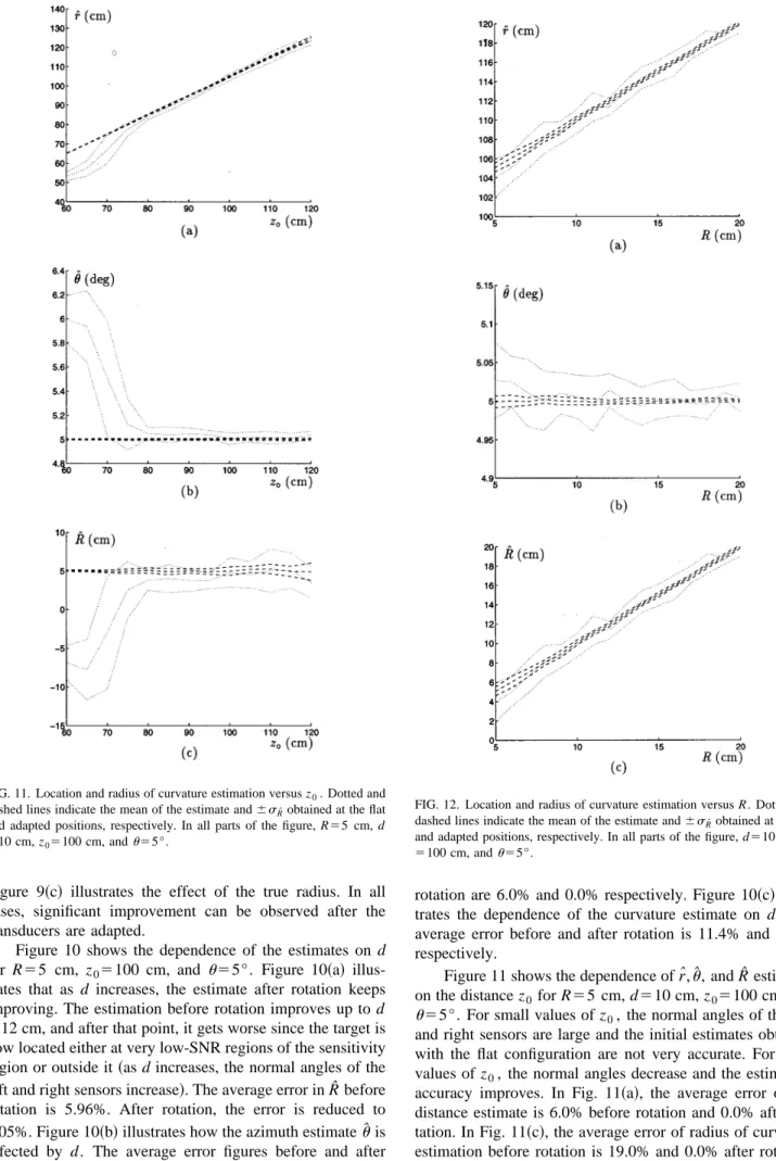
In all of the simulations, a 100-realization Monte-Carlo study has been employed. Figure 9~a! illustrates the effect of varying d on the curvature estimate before and after the transducers are rotated. Note the reduction in the standard deviations of the estimates as d is increased. For d.21 cm, all of the transducers cannot detect the object and the esti-mates become very erroneous. Figure 9~b! illustrates that as

z0 increases, standard deviations of both estimates increase.

FIG. 9. Estimated radius versus~a! d, ~b! z0, and~c! R. Dotted and dashed

lines indicate the mean of the estimate and6sRˆ obtained at the flat and

adapted positions, respectively. In part~a!, R55 cm, z05100 cm. In part

~b!, R55 cm, d510 cm. In part ~c!, d520 cm, z05100 cm.

FIG. 10. Location and radius of curvature estimation versus d. Dotted and dashed lines indicate the mean of the estimate and6sRˆobtained at the flat

and adapted positions respectively. In all parts of the figure, R55 cm, z0

Figure 9~c! illustrates the effect of the true radius. In all cases, significant improvement can be observed after the transducers are adapted.

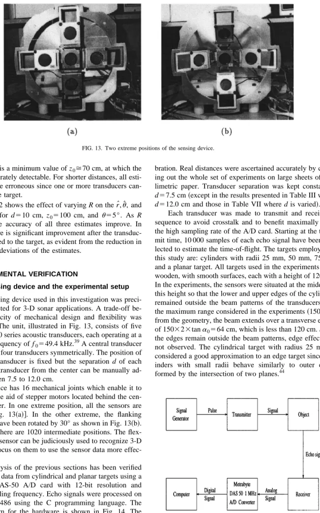
Figure 10 shows the dependence of the estimates on d for R55 cm, z05100 cm, and u55°. Figure 10~a! illus-trates that as d increases, the estimate after rotation keeps improving. The estimation before rotation improves up to d

512 cm, and after that point, it gets worse since the target is

now located either at very low-SNR regions of the sensitivity region or outside it~as d increases, the normal angles of the left and right sensors increase!. The average error in Rˆ before rotation is 5.96%. After rotation, the error is reduced to 0.05%. Figure 10~b! illustrates how the azimuth estimateuˆ is affected by d. The average error figures before and after

rotation are 6.0% and 0.0% respectively. Figure 10~c! illus-trates the dependence of the curvature estimate on d. The average error before and after rotation is 11.4% and 1.2%, respectively.

Figure 11 shows the dependence of rˆ,uˆ , and Rˆ estimates on the distance z₀for R55 cm, d510 cm, z₀5100 cm, and

u55°. For small values of z0, the normal angles of the left and right sensors are large and the initial estimates obtained with the flat configuration are not very accurate. For large values of z0, the normal angles decrease and the estimation accuracy improves. In Fig. 11~a!, the average error of the distance estimate is 6.0% before rotation and 0.0% after ro-tation. In Fig. 11~c!, the average error of radius of curvature estimation before rotation is 19.0% and 0.0% after rotation.

FIG. 11. Location and radius of curvature estimation versus z0. Dotted and

dashed lines indicate the mean of the estimate and6sRˆobtained at the flat

and adapted positions, respectively. In all parts of the figure, R55 cm, d 510 cm, z05100 cm, andu55°.

FIG. 12. Location and radius of curvature estimation versus R. Dotted and dashed lines indicate the mean of the estimate and6sRˆobtained at the flat

and adapted positions, respectively. In all parts of the figure, d510 cm, z0

Again, there is a minimum value of z₀>70 cm, at which the target is accurately detectable. For shorter distances, all esti-mates become erroneous since one or more transducers can-not detect the target.

Figure 12 shows the effect of varying R on the rˆ,uˆ , and

Rˆ estimates for d510 cm, z05100 cm, and u55°. As R increases, the accuracy of all three estimates improve. In addition, there is significant improvement after the transduc-ers are adapted to the target, as evident from the reduction in the standard deviations of the estimates.

VI. EXPERIMENTAL VERIFICATION

A. The sensing device and the experimental setup

The sensing device used in this investigation was preci-sion constructed for 3-D sonar applications. A trade-off be-tween simplicity of mechanical design and flexibility was established. The unit, illustrated in Fig. 13, consists of five Polaroid 6500 series acoustic transducers, each operating at a resonance frequency of f0549.4 kHz.

39

A central transducer is flanked by four transducers symmetrically. The position of the central transducer is fixed but the separation d of each surrounding transducer from the center can be manually ad-justed between 7.5 to 12.0 cm.

The device has 16 mechanical joints which enable it to move with the aid of stepper motors located behind the cen-tral transducer. In one extreme position, all the sensors are coplanar @Fig. 13~a!#. In the other extreme, the flanking transducers have been rotated by 30° as shown in Fig. 13~b!. In between, there are 1020 intermediate positions. The flex-ibility of the sensor can be judiciously used to recognize 3-D targets and focus on them to use the sensor data more effec-tively.

The analysis of the previous sections has been verified by real sonar data from cylindrical and planar targets using a 4-channel DAS-50 A/D card with 12-bit resolution and 1 MHz sampling frequency. Echo signals were processed on an IBM-PC 486 using the C programming language. The block diagram for the hardware is shown in Fig. 14. The experiments were conducted in 2-D to allow accurate

cali-bration. Real distances were ascertained accurately by carry-ing out the whole set of experiments on large sheets of mil-limetric paper. Transducer separation was kept constant at

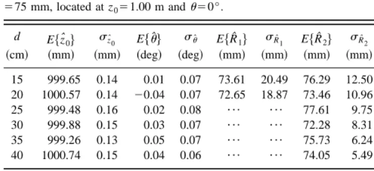
d57.5 cm ~except in the results presented in Table III where d512.0 cm and those in Table VII where d is varied!.

Each transducer was made to transmit and receive in sequence to avoid crosstalk and to benefit maximally from the high sampling rate of the A/D card. Starting at the trans-mit time, 10 000 samples of each echo signal have been col-lected to estimate the time-of-flight. The targets employed in this study are: cylinders with radii 25 mm, 50 mm, 75 mm and a planar target. All targets used in the experiments were wooden, with smooth surfaces, each with a height of 120 cm. In the experiments, the sensors were situated at the middle of this height so that the lower and upper edges of the cylinders remained outside the beam patterns of the transducers. For the maximum range considered in the experiments~150 cm!, from the geometry, the beam extends over a transverse extent of 150323tana₀564 cm, which is less than 120 cm. Since the edges remain outside the beam patterns, edge effects are not observed. The cylindrical target with radius 25 mm is considered a good approximation to an edge target since cyl-inders with small radii behave similarly to outer edges formed by the intersection of two planes.44

FIG. 13. Two extreme positions of the sensing device.

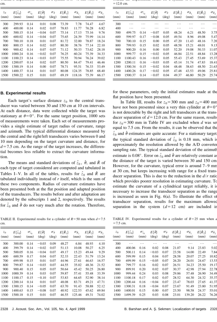
B. Experimental results

Each target’s surface distance z0 to the central trans-ducer was varied between 30 and 150 cm at 10 cm intervals. At each distance, data were collected while the target was stationary at u50°. For the same target position, 1000 sets of measurements were taken. Each set of measurements pro-vides a single estimate of target radius of curvature, range and azimuth. The typical differential distance measured by the central and the right/left transducers varies between 0 and 10 mm depending on the target curvature and distance, for

d57.5 cm. As the range of the target increases, the

differen-tial becomes less reliable to extract the curvature informa-tion.

The means and standard deviations of zˆ0, uˆ , and Rˆ of each type of target considered are computed and tabulated in Tables I–V. In all of the tables, results for zˆ0 and Rˆ are tabulated individually instead of r itself, which is the sum of these two components. Radius of curvature estimates have been presented both at the flat position and adapted position of the transducers. The results before and after adaptation are denoted by the subscripts 1 and 2, respectively. The results for zˆ0 anduˆ do not vary much after the rotation. Therefore,

for these parameters, only the initial estimates made at the flat position have been presented.

In Table III, results for z05300 mm and z05400 mm have not been presented since a very thin cylinder atu50° is not detectable by the right and left transducers at the trans-ducer separation of d512.0 cm. For the same reason, results for z05300 mm in Table IV are excluded when d was set equal to 7.5 cm. From the results, it can be observed that the

zˆ0 anduˆ estimates are quite accurate: For a stationary target, the typical standard deviation of zˆ0 is 0.18 mm, which is approximately the resolution allowed by the A/D converter sampling rate. The typical standard deviation of the azimuth estimate is 0.08°. Error on zˆ0anduˆ are relatively constant as the distance of the target is varied between 30 and 150 cm. However, for the curvature, typical error is around 7–9 mm at 30 cm, but keeps increasing with range for a fixed trans-ducer separation. This is due to the reduction in the d/r ratio which provides poorer resolution in estimating curvature. To estimate the curvature of a cylindrical target reliably, it is necessary to increase the transducer separation as the range is increased as seen in Fig. 6~a!. To illustrate the effect of transducer separation, results for the maximum allowed separation in the system (d512 cm! are included in

TABLE I. Experimental results for a cylinder of R575 mm when d57.5 cm. z0 E$zˆ0% szˆ0 E$uˆ% suˆ E$Rˆ1% sRˆ1 E$Rˆ2% sRˆ2 ~mm! ~mm! ~mm! ~deg! ~deg! ~mm! ~mm! ~mm! ~mm! 300 299.93 0.14 0.01 0.08 73.39 7.78 74.47 4.67 400 400.00 0.14 0.02 0.07 78.83 11.77 76.28 6.82 500 500.15 0.14 20.04 0.07 75.14 17.13 75.16 9.76 600 600.02 0.14 20.04 0.07 75.65 24.39 75.99 14.14 700 700.10 0.18 0.01 0.07 81.72 32.00 78.87 18.24 800 800.15 0.14 0.02 0.07 80.30 38.76 77.14 22.10 900 900.42 0.14 0.07 0.07 71.12 50.33 73.62 28.18 1000 1000.24 0.16 20.02 0.07 76.25 60.24 75.39 34.33 1100 1100.23 0.14 20.03 0.07 75.55 70.94 76.24 39.02 1200 1200.07 0.14 0.02 0.07 80.50 84.47 79.41 46.46 1300 1300.19 0.14 0.00 0.07 78.71 95.51 76.33 53.49 1400 1400.37 0.14 0.01 0.07 80.08 124.35 78.85 68.40 1500 1500.22 0.15 0.01 0.07 69.19 118.16 75.39 66.17

TABLE II. Experimental results for a cylinder of R550 mm when d57.5 cm. z0 E$zˆ0% szˆ0 E$uˆ% suˆ E$Rˆ1% sRˆ1 E$Rˆ2% sRˆ2 ~mm! ~mm! ~mm! ~deg! ~deg! ~mm! ~mm! ~mm! ~mm! 300 300.00 0.14 20.03 0.09 48.27 6.84 48.93 4.10 400 399.79 0.14 20.02 0.07 51.13 10.08 50.27 6.25 500 500.05 0.16 20.04 0.07 49.17 15.23 49.44 9.29 600 600.59 0.17 0.04 0.07 52.33 22.43 51.79 13.24 700 699.98 0.15 0.01 0.07 44.96 27.61 46.63 16.57 800 799.87 0.14 20.03 0.07 44.55 35.02 48.36 21.52 900 900.40 0.15 0.05 0.07 50.64 45.42 50.25 26.80 1000 1000.39 0.14 0.03 0.07 59.87 57.41 55.48 33.39 1100 1100.17 0.15 20.10 0.07 53.83 64.65 52.90 38.14 1200 1200.14 0.14 0.01 0.07 48.08 83.71 49.21 47.71 1300 1300.15 0.14 20.05 0.07 63.70 91.43 58.88 52.12 1400 1400.63 0.15 20.08 0.07 40.92 122.53 45.62 69.84 1500 1500.18 0.15 0.01 0.07 46.55 125.46 49.31 74.02

TABLE III. Experimental results for a cylinder of R550 mm with d 512.0 cm. z0 E$zˆ0% szˆ0 E$uˆ% suˆ E$Rˆ1% sRˆ1 E$Rˆ2% sRˆ2 ~mm! ~mm! ~mm! ~deg! ~deg! ~mm! ~mm! ~mm! ~mm! 300 ¯ ¯ ¯ ¯ ¯ ¯ ¯ ¯ 400 ¯ ¯ ¯ ¯ ¯ ¯ ¯ ¯ 500 499.75 0.14 20.07 0.05 48.24 6.21 48.50 3.75 600 599.97 0.17 20.08 0.05 49.54 8.96 49.08 5.47 700 700.10 0.15 0.00 0.05 47.20 11.43 48.16 7.20 800 799.93 0.15 0.02 0.05 48.58 15.21 48.01 9.13 900 900.20 0.16 0.00 0.05 52.20 19.08 50.33 11.07 1000 999.77 0.15 20.02 0.05 46.84 22.51 48.84 13.28 1100 1100.43 0.16 20.03 0.05 55.43 27.45 53.69 15.37 1200 1200.11 0.16 20.03 0.05 45.14 31.74 47.83 18.41 1300 1300.34 0.15 20.02 0.04 48.48 38.63 48.50 21.63 1400 1400.26 0.17 20.02 0.05 47.48 43.53 49.06 25.81 1500 1500.37 0.14 20.07 0.04 49.37 46.80 50.29 25.74

TABLE IV. Experimental results for a cylinder of R525 mm when d 57.5 cm. z0 E$zˆ0% szˆ0 E$uˆ% suˆ E$Rˆ1% sRˆ1 E$Rˆ2% sRˆ2 ~mm! ~mm! ~mm! ~deg! ~deg! ~mm! ~mm! ~mm! ~mm! 300 ¯ ¯ ¯ ¯ ¯ ¯ ¯ ¯ 400 400.06 0.16 0.02 0.08 21.07 9.14 23.83 5.02 500 500.11 0.14 20.03 0.07 23.58 14.00 22.49 7.84 600 599.99 0.15 0.04 0.07 28.58 20.07 27.25 10.82 700 699.99 0.15 20.05 0.07 26.20 26.01 24.67 13.53 800 799.77 0.16 0.02 0.07 26.51 34.23 25.50 19.17 900 899.91 0.20 0.02 0.07 30.37 42.98 27.94 22.78 1000 999.44 0.24 0.03 0.08 29.86 57.48 26.90 34.49 1100 1100.18 0.17 0.02 0.07 28.52 64.30 24.32 35.37 1200 1200.44 0.16 20.04 0.07 23.47 78.03 27.65 41.37 1300 1300.31 0.18 20.04 0.07 23.67 91.49 23.80 51.95 1400 1400.01 0.15 0.00 0.07 23.50 98.58 24.37 55.01 1500 1499.39 0.25 0.03 0.08 23.01 139.20 26.22 76.26

Table III. Compared to Table II where d57.5 cm, it is ob-served that errors in the radius of curvature estimate are ap-proximately reduced by 60%. In Table V, results for a planar target (R5`) are illustrated. In the experiments, whenever the denominator of Eq.~10! is zero, a very large value (1020) is assigned to R to be able to represent it numerically.

In Table VI, results for the cylinder with R525 mm are provided foru50°,3°,5°,8°. It is observed that the accura-cies of range and azimuth estimates do not change signifi-cantly as compared to the case when the target is along the line-of-sight. The accuracy of the initial curvature estimate degrades with uuu as expected. However, the estimates with the adapted configuration for target at differentu are compa-rable in accuracy. For larger values of u than considered in the table, it is not possible to estimate the curvature since the target will be outside the sensitivity region of either the right or the left transducer.

Finally, the transducers were detached from the mount-ing and were placed on polyamid stands so that larger trans-ducer separations than allowed by the prototype system could be tested (d: 15.0–30.0 cm!. The results are presented in Table VII. When d.21 cm, it is not possible to acquire data with the side transducers at the flat position since the target at z051.00 m remains outside the joint sensitivity re-gion of the transducers. Therefore, for these cases, the trans-ducers are maintained approximately perpendicular to the object surface while experimental data are being collected.

Overall, the results indicate that the accuracy of the cur-vature estimation after adapting the transducers brings an improvement varying between 35% and 45%.

VII. DISCUSSION AND CONCLUSION

A sensing device capable of estimating the location and radius of curvature of spherical and cylindrical targets has been described. The main goal of the study is to assess the performance of radius of curvature estimation. The estima-tion accuracy can be improved by employing an adaptive sensor configuration: After acquiring the initial data, trans-ducers are rotated to align their line-of-sights with the object. This way, SNR is increased and more nearly accurate esti-mates can be obtained. Two limiting cases are of special interest: the point ~in 3-D! or line ~in 2-D! target and the planar target. Analytical results are verified by real sonar data from cylindrical and planar targets. Typical accuracies in range and azimuth are 0.18 mm and 0.1°, respectively. Accuracy of the curvature estimate depends on the target type and system parameters such as transducer separation and operating range. The estimation with the adapted con-figuration gives much better results than without adaptation, and brings an improvement in the accuracy of about 40%.

The radius of curvature estimation provides valuable in-formation for differentiating reflectors with different radii

~including R50 for an edgelike reflector to R5` for a

pla-nar reflector!. The classification procedure, consistent with the experimental results, is illustrated in Fig. 15. The uncer-tainty region of each radius estimate is considered to be be-tween @Rˆ23sRˆ,Rˆ13sRˆ# assuming zero-mean Gaussian-distributed estimation error. The standard deviation sR increases with the radius of curvature. Given two targets with constant curvature, if there is overlap between their uncer-tainty regions, then these targets may not be distinguished for estimates which fall within the overlap region, shown by

TABLE V. Experimental results for a planar target of R5` when d57.5 cm. z0 E$zˆ0% szˆ0 E$uˆ% suˆ E$Rˆ1%5E$Rˆ2% sRˆ15sRˆ2 ~mm! ~mm! ~mm! ~deg! ~deg! ~mm! ~mm! 300 299.88 0.14 20.02 0.08 4.7031018 _2.1231019 400 399.94 0.14 0.01 0.08 1.3031019 _3.3631019 500 500.09 0.15 20.04 0.08 8.0031018 _2.7231019 600 600.11 0.16 20.01 0.07 1.4231019 _3.4931019 700 699.98 0.16 20.02 0.08 1.5331019 _3.6031019 800 800.24 0.15 20.06 0.08 8.0031018 2.7131019 900 899.83 0.17 0.03 0.08 1.0831019 3.1031019 1000 1000.07 0.15 0.03 0.08 1.2531019 3.3131019 1100 1100.18 0.16 0.04 0.08 1.2331019 3.2831019 1200 1199.92 0.17 20.04 0.08 7.9031018 2.7031019 1300 1300.00 0.18 20.05 0.08 9.2031018 2.8931019 1400 1399.80 0.15 20.02 0.08 1.3631019 _3.4331019 1500 1500.34 0.20 0.00 0.08 1.0731019 _3.0931019

TABLE VI. Experimental results for a cylinder with R525 mm for varying

uwhen d57.5 cm.

u E$zˆ0% szˆ0 E$uˆ% suˆ E$Rˆ1% sRˆ1 E$Rˆ2% sRˆ2

~deg! ~mm! ~mm! ~deg! ~deg! ~mm! ~mm! ~mm! ~mm! 0 1000.26 0.16 20.04 0.07 22.65 56.81 24.64 30.60 3 999.46 0.15 2.73 0.08 24.57 58.50 26.77 31.92 5 1000.67 0.15 4.98 0.07 25.64 61.16 23.43 29.75 8 1000.05 0.16 7.53 0.07 27.34 63.34 25.06 31.42

TABLE VII. Experimental results for varying d for a cylinder of radius R 575 mm, located at z051.00 m andu50°. d _E$zˆ0% szˆ₀ E$uˆ% suˆ E$Rˆ1% sRˆ1 E$Rˆ2% sRˆ2 ~cm! ~mm! ~mm! ~deg! ~deg! ~mm! ~mm! ~mm! ~mm! 15 999.65 0.14 0.01 0.07 73.61 20.49 76.29 12.50 20 1000.57 0.14 20.04 0.07 72.65 18.87 73.46 10.96 25 999.48 0.16 0.02 0.08 ¯ ¯ 77.61 9.75 30 999.88 0.15 0.03 0.07 ¯ ¯ 72.28 8.31 35 999.26 0.13 0.05 0.07 ¯ ¯ 75.73 6.24 40 1000.74 0.15 0.04 0.06 ¯ ¯ 74.05 5.49

hatched areas in Fig. 15. The results presented allow such decisions to be based on a solid footing.

For reliable curvature estimation, it is necessary to in-crease the transducer separation as the range is inin-creased. The transducer separation in the present system is relatively limited and not capable of real-time dynamic adaptation. A system which is adaptive also in this respect would be able to maintain high accuracy over a broader range of distances.

When dealing with shapes more general than cylinders and spheres, such as ellipsoidal surfaces, the geometry will be slightly more complicated. Nevertheless, a similar ap-proach can be taken, possibly requiring additional sensors, or sensors with greater capability of motion. Finally, although the method has been developed for convex (R.0) reflectors, it is equally applicable to concave (R,0) reflectors. Targets that have spatially varying curvature which may become both concave and convex have also been addressed in recent work.45,46Naturally, the larger the number of parameters~or degrees of freedom! of the surface, the larger the number of sensors needed.

ACKNOWLEDGMENTS

This work was supported by TU¨ BI˙TAK under Project No. EEEAG-92 and the British Council Academic Link Pro-gram. The authors would like to thank the anonymous re-viewers for their comments.

1

G. C. Carter and E. R. Robinson, ‘‘Ocean effects on time-delay estimation requiring adaptation,’’ IEEE J. Ocean Eng. 18, 367–378~1993!.

2_{A. C. Smith and G. C. L. Searle, ‘‘Empirical observations of a sonar}

adaptive array,’’ IEE Proc. F, Commun. Radar Signal Process. 132, 595– 597~1985!.

3

K. Scarbrough, G. C. Carter, and R. J. Tremblay, ‘‘Performance predic-tions for coherent and incoherent processing techniques of time-delay es-timation,’’ IEEE Trans. Acoust., Speech, Signal Process. 31, 1191–1196 ~1983!.

4

G. C. Carter, ‘‘Coherence and time-delay estimation,’’ Proc. IEEE 75, 236–255~1987!.

5_{M. Wazenski and D. Alexandrou, ‘‘Active, wideband detection and}

local-ization in an uncertain multipath environment,’’ J. Acoust. Soc. Am. 101, 1961–1970~1997!.

6

D. J. W. Hardie and A. B. Gallaher, ‘‘Review of numerical methods for predicting sonar array performance,’’ IEE Proc. F, Radar Sonar and Navi-gation 143, 196–203~1996!.

7_{R. Smith, A. Stevens, A. Frost, and P. Probert, ‘‘Developing a}

sensor-based underwater navigation system,’’ Int. J. Syst. Sci. 29, 1145–1155 ~1998!.

8_{W. K. Stewart, ‘‘3-dimensional stochastic modeling using sonar sensing}

for undersea robotics,’’ Autonomous Robots 3, 121–143~1996!.

9_{R. Kuc, ‘‘Three-dimensional tracking using qualitative bionic sonar,’’}

Ro-botics Autonomous Syst. 11, 213–219~1993!.

10_{M. L. Hong and L. Kleeman, ‘‘Ultrasonic classification and location of}

3-D room features using maximum likelihood estimation II,’’ Robotica

15, 645–652~1997!.

11

L. Kleeman and H. Akbarally, ‘‘A sonar sensor for accurate 3-D target localization and classification,’’ in Proceedings IEEE International

Con-ference on Robotics and Automation, Nagoya, Japan, May 21–27~IEEE,

Piscataway, NJ, 1995!, pp. 3003–3008.

12_{H. Peremans, K. Audenaert, and J. M. Van Campenhout, ‘‘A}

high-resolution sensor based on tri-aural perception,’’ IEEE Trans. Rob. Au-tom. 9, 36–48~1993!.

13_{A. M. Sabatini, ‘‘Statistical estimation algorithms for ultrasonic detection}

of surface features,’’ in Proceedings IEEE/RSJ International Conference

on Intelligent Robots and Systems, Munich, Germany, September 12–16

~IEEE, Piscataway, NJ, 1994!, pp. 1845–1852.

14_{A. M. Sabatini, ‘‘Sampled baseband correlators for in-air ultrasonic}

rangefinders,’’ IEEE Trans. Ind. Electron. 45, 341–350~1998!.

15_{M. K. Brown, ‘‘The extraction of curved surface features with generic}

range sensors,’’ Int. J. Robotics Res. 5, 3–18~1986!.

16_{R. Kuc, ‘‘Biologically motivated adaptive sonar system,’’ J. Acoust. Soc.}

Am. 100, 1849–1854~1996!.

17

R. Kuc, ‘‘Biomimetic sonar recognizes objects using binaural informa-tion,’’ J. Acoust. Soc. Am. 102, 689–696~1997!.

18_{A. Hilton, J. Illingworth, and T. Windeatt, ‘‘Statistics of surface curvature}

estimates,’’ Pattern Recogn. 28, 1201–1221~1995!.

19_{I. E. Dror, M. Zagaeski, and C. F. Moss, ‘‘3-dimensional target}

recogni-tion via sonar—a neural network model,’’ Neural Networks 8, 149–160 ~1995!.

20_{J. A. Simmons, P. A. Saillant, J. M. Wotton, T. Haresign, M. J.}

Fer-ragamo, and C. F. Moss, ‘‘Composition of biosonar images for target recognition by echolocating bats,’’ Neural Networks 8, 1239–1261 ~1995!.

21_{H. L. Roitblat, W. W. L. Au, P. E. Nachtigall, R. Shizumura, and G.}

Moons, ‘‘Sonar recognition of targets embedded in sediment,’’ Neural Networks 8, 1263–1273~1995!.

22_{R. P. Gorman and T. J. Sejnowski, ‘‘Learned classification of sonar targets}

using a massively parallel network,’’ IEEE Trans. Acoust., Speech, Signal Process. 36, 1135–1140~1998!.

23_{T. Ogawa, K. Kameyama, R. Kuc, and Y. Kosugi, ‘‘Source localization}

with network inversion using an answer-in-weights scheme,’’ IEICE Trans. Inf. Syst. E79-D, 608–619~1996!.

24_{W. W. L. Au, ‘‘Comparison of sonar discrimination—dolphin and}

artifi-cial neural network,’’ J. Acoust. Soc. Am. 95, 2728–2735~1994!.

25_{W. Chang, B. Bosworth, and G. C. Carter, ‘‘Results of using an artificial}

neural network to distinguish single echoes from multiple sonar echoes,’’ J. Acoust. Soc. Am. 94, 1404–1408~1993!.

26_{V. Tonard and J. Chatillon, ‘‘Acoustical imaging of extended targets by}

means of synthetic-aperture sonar technique,’’ Acustica 83, 992–999 ~1997!.

27_{S. Stergiopoulos, ‘‘Implementation of adaptive and synthetic-aperture}

pro-cessing schemes in integrated active-passive sonar systems,’’ Proc. IEEE

86, 358–396~1998!.

28_{J. Zemanek, ‘‘Beam behavior within the nearfield of a vibrating piston,’’}

J. Acoust. Soc. Am. 49, 181–191~1971!.

29_{A. D. Pierce, Acoustics, An Introduction to Its Physical Principles and}

Applications~McGraw-Hill, New York, 1981!.

30_{P. M. Morse and K. U. Ingard, Theoretical Acoustics~McGraw-Hill, New}

York, 1968!.

31_{L. W. Camp, Underwater Acoustics ~Wiley-Interscience, New York,}

1970!, Chap. 7, p. 166.

32_{O¨ . Bozma and R. Kuc, ‘‘Characterizing pulses reflected from rough}

sur-faces using ultrasound,’’ J. Acoust. Soc. Am. 89, 2519–2531~1991!.

33_{B. Ayrulu and B. Barshan, ‘‘Identification of target primitives with}

mul-tiple decision-making sonars using evidential reasoning,’’ Int. J. Robotics Res. 17, 598–623~1998!.

34

B. Ayrulu, ‘‘Classification of target primitives with sonar using two non-parametric data-fusion methods,’’ Master’s thesis, Bilkent University, De-partment of Electrical Engineering, Ankara, Turkey, July 1996.

35_{B. Barshan and R. Kuc, ‘‘A bat-like sonar system for obstacle}

localiza-tion,’’ IEEE Trans. Syst. Man Cybern. 22, 636–646~1992!.

36_{B. Barshan, A sonar-based mobile robot for batlike prey capture, Ph.D.}

thesis, Yale University, Department of Electrical Engineering, New Ha-ven, CT, December 1991. University of Michigan Microfilms, order num-ber 9224325.

37_{W. H. Press, B. P. Flannery, S. A. Teukolsky, and W. T. Vetterling,}

Numerical Recipes in Pascal ~Cambridge University Press, Cambridge,

1989!, pp. 574–579.

38_{B. Barshan and B. Ayrulu, ‘‘Performance comparison of four methods of}

time-of-flight estimation for sonar waveforms,’’ Electron. Lett. 34, 1616– 1617~1998!.

39_{Polaroid Corporation, ‘‘Ultrasonic components group,’’ 119 Windsor St.,}

Cambridge, MA 02139~1990!.

40_{B. Barshan and O. Arıkan, ‘‘Performance analysis of two linear array}

processing algorithms for point-obstacle localization,’’ in Proceedings

SPIE Signal and Data Processing of Small Targets, San Diego, CA, July 11–13, 1995, edited by O. E. Drummond~SPIE, Bellingham, WA, 1995!,

Vol. 2561, pp. 533–544.

41_{M. L. Hong and L. Kleeman, ‘‘Analysis of ultrasonic differentiation of}

three-dimensional corners, edges and planes,’’ in Proceedings IEEE

14, 1992~IEEE Computer Society Press, Los Alamitos, CA 1992!, pp.

580–584.

42_{J. J. Leonard and H. F. Durrant-Whyte, ‘‘Mobile robot localization by}

tracking geometric beacons,’’ IEEE Trans. Rob. Autom. 7, 376–382 ~1991!.

43_{B. Barshan and R. Kuc, ‘‘Differentiating sonar reflections from corners}

and planes by employing an intelligent sensor,’’ IEEE Trans. Pattern. Anal. Mach. Intell. 12, 560–569~1990!.

44

R. Kuc and M. W. Siegel, ‘‘Physically-based simulation model for

acous-tic sensor robot navigation,’’ IEEE Trans. Pattern. Anal. Mach. Intell.

PAMI-9, 766–778~1987!.

45_{D. Bas¸kent and B. Barshan, ‘‘Morphological surface profile extraction}

from multiple sonars,’’ in Proceedings of the 1998 IEEE/RSJ

Interna-tional Conference on Intelligent Robots and Systems, Victoria, B.C.,

Canada, October 1998~IEEE, Piscataway, NJ, 1998!, pp.1515–1520.

46

D. Bas¸kent and B. Barshan, ‘‘Surface profile determination from multiple sonar data using morphological processing,’’ Int. J. Robotics Res., in press.