The combined use of wavelet transform and black box models
in reservoir inflow modeling
Umut Okkan
1 *, Zafer Ali Serbes
21 Department of Civil Engineering, Balikesir University, Balikesir, Turkey.
2 Department of Farm Structures and Irrigation, Ege University, Izmir, Turkey; E-mail: [email protected] * Corresponding Author. Phone: 0090 0266 612 11 94-95. E-mail: [email protected]
Abstract: In the study presented, different hybrid model approaches are proposed for reservoir inflow modeling from the meteorological data (monthly precipitation, one-month-ahead precipitation and monthly mean temperature data) by the combined use of discrete wavelet transform (DWT) and different black box techniques. Multiple linear regression (MLR), feed forward neural networks (FFNN) and least square support vector machines (LSSVM) were considered as the black box methods. In the modeling strategy, meteorological input data were decomposed into wavelet sub-time se-ries at three resolution levels and ineffective sub-time sese-ries were eliminated by Mallows’ Cp based all possible
regres-sion method. As a result of all possible regresregres-sion analyses, 2-months mode of time series of monthly temperature (D1_Tt), 8-months mode of time series (D3_Tt) of monthly temperature and approximation mode of time series (A3_Tt)
of monthly temperature were eliminated. Remained effective sub-time series were used as the inputs of MLR, FFNN and LSSVM. When the performances of the training and testing periods were compared, it was observed that the DWT-FFNN conjunction model has better results in terms of mean square errors (MSE) and determination coefficients (R2)
statistics. The discrete wavelet transform approach also increased the accuracy of multiple linear regression and least squares support vector machines.
Keywords: Hybrid model; Discrete wavelet transform; Mallows’ Cp method; Multiple linear regression; Feed forward
neural networks; Least squares support vector machines; Reservoir inflow modeling. INTRODUCTION
Analyzing inflow data of reservoir can give significant sta-tistical information for both past and future characteristics of a dam. Therefore, recording and modeling of inflow data have highly considerable roles in planning, reservoir operation stud-ies and water resources management. There are three main approaches that have been used flow modeling which include white-box model (physically based distributed models), gray-box model (conceptual models) and the black-gray-box model. The white and gray-box models aim to simulate the physical mech-anisms underlying each component in the transformation of rainfall into flow, such as surface, subsurface and groundwater flow. Yet, due to their data requirements, uncertainties and complexities, these models may not be readily used in some applications (Abbott and Refsgaard, 1996).
A basin can also be represented by black-box models which associate basin inputs and desired outputs without detailed considerations on the physical processes. In this context, con-ventional statistical models such as linear-nonlinear regression types and stochastic models were commonly used. There are some important references which provide detailed descriptions of these conventional statistical models for hydrology context (Salas et al., 1980).
Over the past decade, artificial intelligence methods have been widely used as black-box technique in the modeling stud-ies. Especially, artificial neural networks (ANN), which is a nonlinear computing artificial intelligence technique inspired by the learning function of a human brain, have been used in many applications. There are numerous ANN applications with different algorithms in hydrology context (Campolo et al., 1999; Cigizoglu, 2005; Coulibaly et al., 2000; Razavi and Araghinejad, 2009). In addition to ANN, support vector ma-chines (SVM) which is one of the artificial intelligence
meth-ods has been also successfully applied (Bray and Han, 2004; Cimen, 2008; Lin et al., 2006; Liong and Sivapragasam, 2002; Okkan, 2012).
Although some artificial intelligence methods had been used extensively as useful tools for modeling, it has also some prob-lems to deal with non-stationary data. As the hydrological time series includes several frequency components and have nonlin-ear relationships, some hybrid models which include different data-preprocessing and statistical techniques (set pair analysis, principle component analysis, clustering methods) have been used to raise the modeling performance (Wang et al., 2006; Wu et al., 2008).
Recently, an alternative data-preprocessing technique called wavelet transform has been found to be popular in modeling studies due to its advantages over conventional methods. There are several applications of the combined use of wavelet trans-form-neural networks (Anctil and Tape, 2004; Wang and Ding, 2003; Wang et al., 2009), wavelet transform-multiple regres-sion (Kucuk and Agiralioglu, 2006), wavelet transform - sup-port vector machine (Kisi and Cimen, 2011). In addition to flow modeling, wavelet transform was also applied to the analysis of lake levels. Cengiz (2011) investigated the variability of lake levels in four lakes in the Great Lakes region by using wavelet transform and global spectra method. It was showed that lake levels periodicities were generally the annual cycle.
In this study, three hybrid models are proposed for reservoir inflow modeling from the monthly meteorological data by using wavelet transform and some black box approaches (mul-tiple linear regression, feed forward neural networks and least square support vector machines). Firstly, meteorological data were decomposed into wavelet sub-time series. Later, explana-tory sub-time series were determined by using all possible regression method. These predictors constituted the inputs of these black box models.
METHODS
Feed forward neural networks (FFNN)
There are some books which provide a detailed description of the FFNN (Ham and Kostanic, 2001), and hence only a brief description of FFNN is given here. The running procedure of FFNN involves typically two phases; forward computing and backward computing.
In forward computing, each layer uses a weight matrix asso-ciated with all the connections made from the previous layer to the next layer.
The hidden layer has the weight matrix Wij and activation
function f (1); the output layer has the weight matrix W
jm and
activation function f (2). Given the network input vector x ∈Rnx1, the output of the output layer, which is the response (output) of the network y ∈Rmx1, can be written as:
ym= f(2) f(1) x iWij i=1 n ∑ + bj ⎛ ⎝⎜ ⎞ ⎠⎟ ⎡ ⎣ ⎢ ⎤ ⎦ ⎥Wjm+ bm j=1 m ∑ ⎧ ⎨ ⎪ ⎩⎪ ⎫ ⎬ ⎪ ⎭⎪. (1)
After the phase of forward computing, backward computing, which depends on the algorithms to adjust weights, is carried out. The process of adjusting these weights to minimize the differences between the actual and desired output values is called training or learning of network. If these differences (er-rors) are higher than the desired values, the errors are passed backwards through the weights of the network. In ANN termi-nology, this phase is also called the back propagation.
Depending on the techniques to train FFNN models, differ-ent back propagation algorithms have been developed. In this study, the Levenberg-Marquardt back propagation algorithm was used in training of the FFNN. The Levenberg-Marquardt back propagation algorithm is a second-order nonlinear optimi-zation technique that is usually faster and more reliable than any other back propagation techniques (Coulibaly et al., 2000). The Levenberg-Marquardt optimization algorithm represents a simplified version of Newton method applied to the training of FFNN (Hagan and Menhaj, 1994). The training process can be viewed as finding a set of weights that minimize the error (ep)
for all samples in training set (T). The performance function is a sum of squares of the errors as follows:
E(W )=1 2 (dp− yp) 2 p=1 P ∑ =1 2 (ep) 2 p=1 P ∑ , P= mT, (2)
where T is the total number of training samples, m is the num-ber of output layer neurons, W represents the vector containing all the weights in the network, yp is the actual network output, and dp is the desired output.
When training with the Levenberg-Marquardt algorithm, the changing of weights ΔW can be computed as follows:
ΔWk= − [JkTJk+µkI]−1JkTek. (3)
Then, the update of the weights can be adjusted as follows:
Wk+1= Wk+ ΔWk, (4)
where J is the Jacobian matrix, I is the identify matrix, µ is the Marquardt parameter which is to be updated using the decay
rate β depending on the outcome. In particular, µ is multiplied by the decay rate β (0 < β < 1) whenever E(W) decreases, while µ is divided by β whenever E(W) increases in a new step (Cou-libaly et al., 2000; Ham and Kostanic, 2001).
Least squares support vector machines (LSSVM)
The details of standard SVM method were given by Vapnik (1998). In this study, least squares support vector machine (LSSVM), which method is a simplified version of standard SVM, is used in modeling. LSSVM method can be described as fallow according to the studies proposed by Suykens et al. (2002).
Like ANN, a LSSVM model is made up neurons which are organized in two layers. However, unlike ANN, it is based on theory in statistical learning and different error optimization approach (Suykens et al., 2002).
Given n-dimensional input vectorxk∈Rn, the output of the LSSVM model
yk∈R, can be written as:
y = WTφ(x) + b , (5)
where W is weight vector, φ(x) nonlinear mapping function ( φ Rn→ Rnhmapping to high dimensional feature space) and b is the bias term.
Given training set {xk, yk}kN=1, the error optimization prob-lem is defined as:
min J (W ,e)= 1 2W TW+γ 1 2 ek2 k=1 N ∑ , (6)
subject to equality constraints
yk= WTφ(xk)+ b + ek, k= 1,..., N , (7)
where ek is error term and γ regularization parameter.
Because of high dimensional feature space, solution of this optimization problem cannot be obtained by using classical numerical methods. The solution of the optimization problem is obtained by considering the Lagrangian as:
L(W ,b,e,α ) = J(W ,e) − αk W Tφ(x k)+ b + ek− yk
{
}
k=1 N ∑ , (8)where αk are Lagrange multipliers. Conditions for optimality can be obtained by differentiating with respect to W, b, ek and
αk, i.e. ∂L ∂W = 0 → W = αkφ(xk) k=1 N ∑ , (9a) ∂L ∂b= 0 → αk= 0 k=1 N ∑ , (9b) ∂L ∂ek = 0 →αk=γ ek, k= 1,..., N , (9c)
∂L ∂αk= 0 → WTφ(xk)+ b + ek− yk, k= 1,..., N . (9d) Solution 0 1T 1 Ω +γ−1I ⎡ ⎣ ⎢ ⎢ ⎤ ⎦ ⎥ ⎥ b α ⎡ ⎣ ⎢ ⎤ ⎦ ⎥ =⎡0y ⎣ ⎢ ⎤ ⎦ ⎥ (10) with y= [y1;....; yN], 1 = [1;....;1],α = [α1;....;αN] and by apply-ing Mercer’s theorem (Mercer, 1909).
Ωkm=φ(xk)Tφ(xm)= K(xk, xm), k,m= 1,..., N . (11) Resulting LSSVM model for function estimation can be ex-pressed as:
y=k=1αkK(xk, x) N
∑ + b , (12)
where K(xk , x) is the Kernel function.
The Kernel functions treated by standard SVM and LSSVM are the functions with linear, polynomial, Gaussian radial basis, exponential radial basis, splines etc. (Okkan, 2012). The Gauss-ian radial basis function used in this study can be defined as
K(xk, x)= exp − x− xk 2 2σ2 ⎛ ⎝ ⎜ ⎜ ⎞ ⎠ ⎟ ⎟, (13)
where σ is the Gaussian radial basis Kernel function width. Wavelet transform
The wavelet transform, developed during the last decades, is an effective decomposition method. This method provides an analyzing way of a signal in both time and frequency and ap-pears to be a more successful than the conventional Fourier transforms that do not provide time-frequency analysis for the variables involve non-stationary signals (Daubechies, 1990; Kucuk and Agiralioglu, 2006).
The time-scale wavelet transform of a continuous time sig-nal, x(t), is defined as : W (s,τ ) = s−1/2 −∞ ∞ ∫ ψ*⎛⎝⎜t−sτ⎞⎠⎟x(t)dt τ ∈R, s ∈R,s ≠ 0 , (14)
where * corresponds to the complex conjugate and ψ(t) is wavelet function or mother wavelet, s is scale or frequency factor, τ is time factor, R is the domain of real number.
Eq. (14) describes that wavelet transform is the decomposi-tion of x(t) under different resoludecomposi-tion scale. The original series can be reconstructed using the inversion of transform (Rajaee et al., 2011).
In this study, the Haar mother wavelet (simple wavelet) has been used because it is conceptually simple, fast and memory efficient.
The Haar mother wavelet is defined as:
ψ (t) = 1 0≤ t ≤ 1/ 2 −1 1/ 2 ≤ t ≤ 1 0 otherwise ⎧ ⎨ ⎪ ⎩ ⎪ . (15)
For practical applications in hydrology, researchers have ac-cess to a discrete time signal, rather than to a continuous time signal. A discretization of Eq. (14) based on trapezoidal rule is perhaps the simplest discretization of the continuous wavelet transform (CWT). It transform produces N2 coefficients from a data set of length N; hence unnecessary information is locked up within the coefficients; which may or may not be a desirable property. To overcome this difficulty, discrete wavelet trans-forms (DWT) which present power of two logarithmic scaling of the translations can be used in practical applications. Be-cause it reduces the computational complexity of the CWT and the redundancy of the CWT, there is an advantage for prefer-ring the DWT over the CWT (Rajaee et al., 2011).
In this study, the Mallat algorithm was used for the DWT of monthly time-series. According to the Mallat algorithm, the discrete wavelet transform of discrete time series xt is defined
as (Mallat, 1989): Wj,k= 2− j/2 ψ (2− jt− k)x t t=0 N−1 ∑ , (16)
where t is integer time steps, j and k are integers that control, respectively, the scale and time, Wj,k is the wavelet coefficient
for the scale factor s = 2j and the time factor τ = 2jk.
In DWT method, the time series (xi) passes through two
fil-ters and are decomposed into wavelet sub-time series compo-nents, which can be computed by using Eq. (16), without losing the information about the instant of the element occurrence. The DWT converts a signal into father and mother wavelets. Father wavelets represent the high-scale, low frequency com-ponents (approximation (A) comcom-ponents). Mother wavelets are representations of the low-scale, high frequency components (detail (D) components). Thus, DWT allows one to study dif-ferent investing behaviors in difdif-ferent time scales independent-ly (Rajaee et al., 2011). These computations can be carried out by wavelet toolbox for use with MATLAB.
STUDY AREA AND DATA
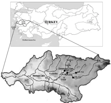
The study area covers the drainage basin of Demirkopru Dam (total drainage area of 6590 km2), which is located in the Gediz basin and Aegean region in Turkey. The reservoir of the dam is fed by four streams. Streamflow is observed at four
gauging stations (Demirci/EIE-522, Deliinis/EIE-515,
Selendi/EIE-514, and Gediz/EIE-523) located upstream of the dam (Fig. 1).
For the study area, the data sets of streamflow (106 m3) were
acquired from the records of the II. Regional Directorate of State Hydraulic Works of Turkey, and were arranged for the period between January 1977 and December 2006. In addition to inflow data, the data sets of precipitation at Demirci, Icikler, Kiransih, Fakili and Gediz meteorological stations were ob-tained from the State Meteorological Organization of Turkey and the General Directorate of State Hydraulic Works of Tur-key. Next, the monthly mean areal precipitation values were calculated from these meteorological stations by Thiessen po-lygons. The monthly data sets of temperature at Demirci and Gediz meteorological stations were also obtained from the State Meteorological Organization of Turkey and the monthly mean
areal temperature values were computed by using arithmetical mean values from these meteorological stations for the period from January 1977 to December 2006.
Fig. 1. Gediz Basin and Demirkopru Dam ( : flow gauging sta-tions; : meteorological stations).
In hydrological modeling, the determination of appropriate input variables would play an important role. In this study, modeling strategy that predicts inflow data from inputs based on monthly rainfall and temperature data. In addition to concur-rent values of input data, precipitation values at various lags were also considered. A statistical approach proposed by Sudheer et al. (2002) was employed to determine the appropri-ate order of precipitation lag. The approach is based on the heuristic that the potential influencing variables corresponding to different time lags can be identified through statistical analy-sis of the data series that uses cross correlation between the variables. The cross correlation function (CCF) between the reservoir inflow and precipitation values at various lags showed significant correlation at concurrent precipitation and one month of precipitation lag on the inflow. Thus, three input data (Pt, Tt, Pt-1) were prepared for the same periods of the monthly
inflow records (Pt: monthly precipitation; Pt-1:
one-month-ahead precipitation; Tt: monthly temperature).
APPLICATION AND RESULTS
In the study presented, DWT was linked to different black box models (MLR, FFNN and LSSVM) for the reservoir inflow modeling. In the modeling strategy, the input data (Pt, Pt-1, Tt)
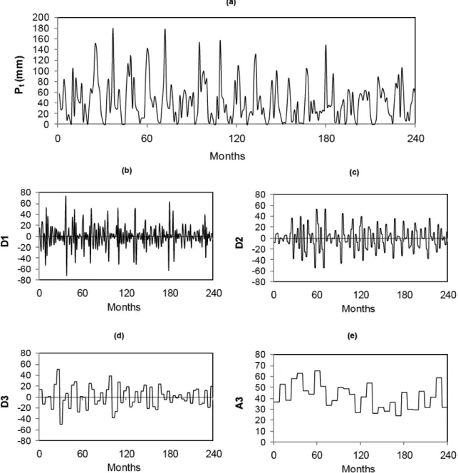
of training and testing periods were decomposed into a certain number of sub-time series components by DWT. In order to decompose the input data, a decomposition level must be se-lected. For the monthly scaled hydrological modeling studies, three decomposition levels are able to represent the related time series (Kisi and Cimen, 2011). Similarly, three decomposition levels were used in this study. Thus, meteorological data were decomposed and twelve sub-time series components (time series of 2-months mode (D1), 4-months mode (D2), 8-months mode (D3) and approximation mode (A3)) were obtained for the training and testing periods by proportions of 2/3 (January 1977−December 1996) and 1/3 (January 1997−December
2006), respectively. For example, the three levels decomposi-tion of the Pt that yield four sub-signals by the Haar wavelet are
presented in Fig. 2.
After the decomposition processes, the effective sub-time se-ries components should be determined as some correlated sub-time series components may reduce the performances of the black box models. In this study, the effective sub-time series components were determined by Mallows’ Cp based all possible
regression method. This statistical method is an effective way to determine the subset of variables in cases where there are a large number of potential predictor variables. In Mallows’ Cp
approach, adequate models are those for which Cp is roughly
equal to the number of variables in the model (Mallows, 1973). The Cp values can be computed as:
Cp= (N − k)MSEi
2
MSEF2− (N − 2i −1) , (17)
where N is the number of data, MSEi is the mean of residual
squares in the model with i variable, MSEF is the mean of
re-sidual squares in the full model with k variable.
Once the effective variables were selected, based on the Cp
values for training period were calculated as shown in Tab. 1. Performances of the models with the nine variables (seen as bold and underlined characters in Tab. 1) are nearly the same as those of the model with twelve variables; that is, the explained variance of the monthly reservoir inflow data by the model with nine variables, which has the minimum Cp value, is nearly
equal to that explained the full linear model with twelve varia-bles. According to the analyses, 2-months mode of time series of monthly temperature (D1_Tt), 8-months mode of time series
of monthly temperature (D3_Tt), and approximation mode of
time series of monthly temperature (A3_Tt ) were eliminated.
Before presenting the input data to FFNN and LSSVM, the all data were normalized in the range [0–1] to prevent the mod-els from being dominated by the variables with the extreme values.
Models with optimum structures provided the best training result in terms of the minimum mean square errors (MSE), and the maximum determination coefficients (R2) were also
em-ployed for the testing period. In the application, some codes which involve discrete wavelet transform and multi-linear regression (DWT-MLR), Levenberg-Marquardt algorithm based feed forward neural networks (DWT-FFNN), least squares support vector machines (DWT-LSSVM) were written in MATLAB. The results of DWT-MLR, DWT-FFNN and DWT-LSSVM models were also compared with conventional MLR, FFNN and LSSVM models. MLR and DWT-MLR coef-ficients were computed by using the variables of training period (January 1977–December 1996). Thus, the testing of models was carried out using determined regression equations.
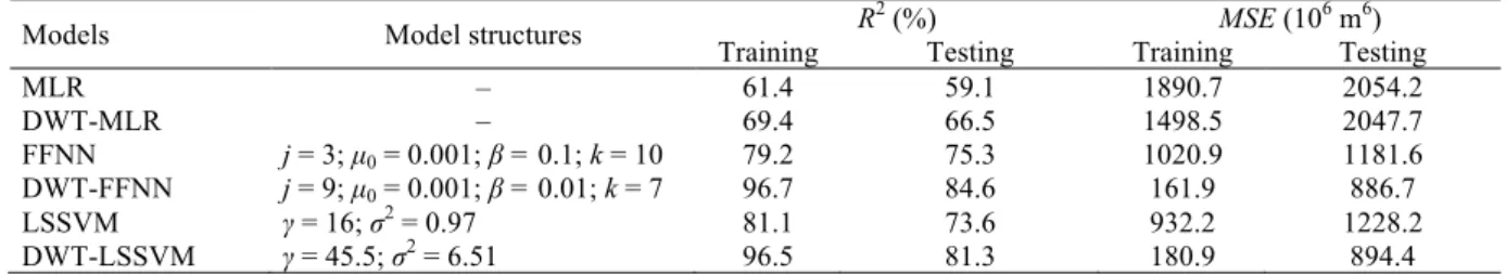
In FFNN applications, three widely used transfer functions, namely tangent sigmoid, linear, and log-sigmoid are evaluated in FFNN structure trials. The best results were achieved by using the log-sigmoid function. The optimum values of LSSVM and DWT-LSSVM parameters were determined by using the trial and error approach. The best configurations of all models are presented in Table 2.
DISCUSSIONS AND CONCLUSIONS
Many of the activities associated with planning and manage-ment of water resources require appropriate hydrological
Fig. 2. Original time series (a), 2-months mode of time series (b), 4-months mode of time series (c), 8-months mode of time series (d) and approximation mode of time series (e) of monthly precipitation for training period.
models in practice. In particular, there is a necessity for model-ing of flow values to optimize the system or to plan for future variations. The current study presented the applications of DWT based black box models (DWT-MLR, DWT-FFNN and DWT-LSSVM) compared with MLR, FFNN and LSSVM models used undecomposed data, for modeling of monthly inflows of Demirkopru Dam, based on the meteorological data. In the study presented, monthly meteorological data (Pt, Pt-1,
Tt) were decomposed into wavelet sub-time series by using the
discrete wavelet transform (DWT). Three resolution levels were considered. Thus, twelve sub-time series components (time series of 2-months mode (D1), 4-months mode (D2), 8-months mode (D3) and approximation mode (A3) for each input data) were determined for the training period and testing period.
Because correlated sub-time series components reduced the generalization capabilities of the models, effective sub-time series components were determined by using Mallows Cp based
all possible regression method. As a result of all possible re-gression analyses, effective sub-time series components were
selected. Thus, these variables that represented the new inputs of the MLR, ANN and LSSVM were treated so as to reduce collinearity.
Table 2 presents the statistical measures performed by the dif-ferent kind of black box models. Because the phenomenon of the hydrological time series have the inherent complexities and nonlinearities, the performance of single MLR model was not suitable. On the contrary, DWT approach increased the perfor-mances of the MLR, FFNN and LSSVM in terms of MSE and R2 values for training and testing periods (Okkan, 2011, 2012).
The model structures with the best accuracy were also provided in Tab. 2. Furthermore, when y = ax + b fitted lines are exam- ined, one can see that for MLR, FFNN, and DWT-LSSVM models, the slope “a” gets closer to one, and “b” gets closer to zero, compared to the conventional MLR, FFNN and LSSVM models.
In terms of the best accuracy, DWT-FFNN model with Haar mother wavelet resulted in MSE reductions and, R2 increases
Table 1. Summary of all possible regression analyses. Number of variables R2 [%] Adj.R2 [%] Cp D1_ Pt D2_ Pt D3_ Pt A3_ Pt D1_ Pt-1 D2_ Pt-1 D3_ Pt-1 A3_ Pt-1 D1_ Tt D2_ Tt D3_ Tt A3_ Tt 1 25.0 24.7 327.8 ● 1 19.0 18.7 373.0 ● 1 17.8 17.5 382.1 ● 2 42.8 42.3 195.9 ● ● 2 39.4 38.9 221.5 ● ● 2 37.5 37.0 236.0 ● ● 3 55.3 54.7 104.2 ● ● ● 3 52.2 51.6 127.6 ● ● ● 3 51.9 51.3 129.7 ● ● ● 4 63.9 63.3 41.1 ● ● ● ● 4 60.8 60.2 64.5 ● ● ● ● 4 60.5 59.9 66.7 ● ● ● ● 5 66.1 65.4 27.0 ● ● ● ● ● 5 64.9 64.2 35.6 ● ● ● ● ● 5 64.8 64.0 37.0 ● ● ● ● ● 6 67.1 66.2 21.5 ● ● ● ● ● ● 6 66.9 66.0 22.9 ● ● ● ● ● ● 6 66.9 66.0 23.0 ● ● ● ● ● ● 7 67.9 66.9 17.4 ● ● ● ● ● ● ● 7 67.9 66.9 17.5 ● ● ● ● ● ● ● 7 67.7 66.7 18.9 ● ● ● ● ● ● ● 8 68.7 67.6 13.4 ● ● ● ● ● ● ● ● 8 68.6 67.5 14.0 ● ● ● ● ● ● ● ● 8 68.4 67.3 15.4 ● ● ● ● ● ● ● ● 9 69.4 68.2 9.9 ● ● ● ● ● ● ● ● ● 9 68.9 67.6 14.1 ● ● ● ● ● ● ● ● ● 9 68.8 67.6 14.3 ● ● ● ● ● ● ● ● ● 10 69.6 68.3 10.6 ● ● ● ● ● ● ● ● ● ● 10 69.6 68.3 10.7 ● ● ● ● ● ● ● ● ● ● 10 69.5 68.1 11.5 ● ● ● ● ● ● ● ● ● ● 11 69.8 68.3 11.4 ● ● ● ● ● ● ● ● ● ● ● 11 69.7 68.2 12.2 ● ● ● ● ● ● ● ● ● ● ● 11 69.6 68.2 12.3 ● ● ● ● ● ● ● ● ● ● ● 12 69.8 68.2 13.0 ● ● ● ● ● ● ● ● ● ● ● ●
Table 2. The performances of different model applications in the training and testing periods.
Models Model structures Training R2 (%) Testing Training MSE (106 mTesting 6)
MLR – 61.4 59.1 1890.7 2054.2 DWT-MLR – 69.4 66.5 1498.5 2047.7 FFNN j = 3; µ0 = 0.001; β = 0.1; k = 10 79.2 75.3 1020.9 1181.6 DWT-FFNN j = 9; µ0 = 0.001; β = 0.01; k = 7 96.7 84.6 161.9 886.7 LSSVM γ = 16; σ2 = 0.97 81.1 73.6 932.2 1228.2 DWT-LSSVM γ = 45.5; σ2 = 6.51 96.5 81.3 180.9 894.4
j is number of neurons in hidden layer, k is iteration number, µ0 is initial Marquardt parameter, β is decay rate of Levenberg-Marquardt algorithm, γ is regularization parameter, σ is Gaussian radial basis kernel function width.
(a) (b)
Fig. 3. The scatter plots (a) and hydrographs (b) of DWT-FFNN model for the testing period.
y = 1.083x + 9.4287 R² = 0.8464 y = x 0 50 100 150 200 250 300 350 400 450 0 50 100 150 200 250 300 350 400 450 DW T -FFN N Observed 0 50 100 150 200 250 300 350 400 01.01.1997 01.01.1999 01.01.2001 01.01.2003 01.01.2005 In flo w s ( 1 0 6m 3) Observed DWT-FFNN
zation capability and thus can more easily capture inflow of Demirkopru Dam. The scatter plot and hydrograph of DWT-FFNN for the testing period are presented in Fig. 3.
Besides of the MSE and R2 values, in terms of descriptive
statistics, DWT-FFNN model proved to be successful in the training and testing periods. It was also seen that the extreme value statistics of DWT-FFNN for the testing period were quite satisfactory providing superior results compared with other conventional methods.
Although DWT-FFNN models have ability to represent complex and nonlinear relations of a basin, the structures of feed forward neural networks (FFNN) may be hard to deter-mine and they can be deterdeter-mined using after many trial-and-error simulations. Therefore, DWT based MLR (DWT-MLR) and DWT based LSSVM (DWT-LSSVM) models that may be much easier for practical interpreting. Thus, these approaches can be used as alternative ways to DWT-FFNN and FFNN methods for monthly reservoir inflow modeling. For example, LSSVM and DWT-LSSVM have considerable features includ-ing the fact that requirement on Kernel function and the nature of the optimization problem results in a uniquely global opti-mum, generalization capability, and avoidance of converging to a local minimum solution.
The study presented uses some hybrid methodologies that are beneficial in reconstruction of reservoir inflow data. Espe-cially, developed DWT-FFNN and DWT-LSSVM models, which are successful tools for the modeling of reservoir inflow series, can be used for future assessment of climate change impacts at the watershed scale. Thus, they can be employed to produce significant monthly scaled information for water re-sources management and planning problems such as irrigation planning, reservoir operation, water budget studies, watershed modeling, etc. The authors also suggest that the developed hybrid techniques can be also applied to other hydrological variables and other water resources problems to reconfirm the effectiveness of them.
In the study, the Mallat algorithm was used for the DWT of monthly meteorological time-series. For future study, the other DWT algorithms (e.g., Trous algorithm) and the other types of transform (e.g., fast wavelet transform, Fourier transform) may be used for the construction of the different neuro-computing models (e.g., other neural network algorithms, fuzzy logic). In addition to these, other data-preprocessing techniques (e.g., principle component analysis, factor analysis, set pair analysis) can be also compared with the wavelet transform for the future researches.
Acknowledgements. Authors feel responsible to thank English Instructor Cuneyt Guren and as well as workers of II. Regional Directorate of State Hydraulic Works and Turkish State Mete-orological Service for their help with data collection. Com-ments from two anonymous reviewers, which have helped to improve the paper, are also acknowledged.
REFERENCES
Abbott, M.B., Refsgaard, J.C., 1996. Distributed Hydrological Modeling. Kluver Academic Publishers, Dordrecht, 17–39. Anctil, F., Tape, D.G., 2004. An exploration of artificial neural
network rainfall-runoff forecasting combined with wavelet decomposition. J. Environmental Engng. and Science, 3, 21– –128.
Bray, M., Han, D., 2004. Identification of support vector ma-chines for runoff modelling. J. Hydroinformatics, 6, 265– –280.
Campolo, M., Andreussi, P., Soldati, A., 1999. River flood forecasting with a neural network model. Water Resour. Res., 35, 1191–1197.
Cengiz, T.M., 2011. Periodic structures of great lakes levels using wavelet analysis. J. Hydrol. Hydromech., 59, 1, 24–35. Cigizoglu, H.K., 2005. Generalized regression neural networks in monthly flow forecasting. Civil Engineering and Envi-ronmental Systems, 22, 2, 71–84.
Cimen, M., 2008. Estimation of daily suspended sediments using support vector machines. Hydrological Sciences Jour-nal, 53, 3, 656–666.
Coulibaly, P., Anctil, F., Bobee, B., 2000. Daily reservoir in-flow forecasting using artificial neural Networks with stopped training approach. J. Hydrol., 230, 244–257. Daubechies, I., 1990. The wavelet transform, time-frequency
localization and signal analysis. IEEE Transactions on In-formation Theory, 36, 5, 961–1005.
Hagan, M.T., Menhaj, M.B., 1994. Training feed forward tech-niques with the Marquardt algorithm. IEEE Transactions on Neural Networks, 5, 6, 989–993.
Ham, F., Kostanic, I., 2001. Principles of Neurocomputing for Science and Engineering. Macgraw-Hill. USA.
Kisi, O., Cimen, M., 2011. A wavelet-support vector machine conjunction model for monthly streamflow forecasting. J. Hydrol., 399, 132–140.
Kucuk, M., Agiralioglu, N., 2006, Wavelet regression tech-nique for streamflow prediction. J. Applied Statistics, 33, 9, 943–960.
Lin, J.Y., Cheng, C.T., Chau, K.W., 2006. Using support vector machines for long-term discharge prediction. Hydrological Sciences J., 51, 4, 599–612.
Liong, S.Y., Sivapragasam, C., 2002. Flood stage forecasting with support vector machines. J. Amer. Water Resources Assoc., 38, 1, 173–186.
Mallat, S.G., 1989. A theory for multi resolution signal decom-position: the wavelet representation. IEEE Transactions on Pattern Analysis and Machine Intelligence, 11, 7, 674–693. Mallows, C.L., 1973. Some comments on Cp. Technometrics,
15, 4, 661–675.
Mercer, J., 1909. Functions of positive and negative type and their connection with the theory of integral equations. Philo-sophical Transactions of the Royal Society, London, 209, 415–446.
Okkan, U., 2011. Application of Levenberg-Marquardt optimi-zation algorithm based multilayer neural networks for hydro-logical time series modeling. An Int. J. Optimization and Control: Theories & Applications, 1, 1, 53–63.
Okkan, U., 2012. Performance of least squares support vector machine for monthly reservoir inflow prediction. Fresenius Environmental Bull., 21, 3, 611–620.
Rajaee, T., Nourani, V., Mohammad, Z.K., Kisi, O., 2011. River suspended sediment load prediction: Application of ANN and wavelet conjunction model. J. Hydrol. Engng, 16, 8, 613–627.
Razavi, S., Araghinejad, S., 2009. Reservoir inflow modeling using temporal neural networks with forgetting factor ap-proach. Water Resour. Management, 23, 39–55.
Salas, J.D., Delleur, J.W., Yevjevich, V., Lane, W.L., 1980. Applied modeling of hydrologic time series. Water Resouces Pub., p. 484.
Sudheer, K.P., Gosain, A.K., Ramasastri, K.S., 2002, A data-driven algorithm for constructing artificial neural network rainfall-runoff models. Hydrol. Processes, 16, 1325–1330.
Suykens, J.A.K., Van Gestel, T., De Brabanter, J., De Moor, B., Vandewalle, J., 2002. Least Squares Support Vector Ma-chines. World Science, Singapore.
Vapnik, V., 1998. Statistical Learning Theory. John Wiley & Sons, Toronto.
Wang, W., Ding, J., 2003. Wavelet network model and its application to the prediction of hydrology. Nature and Sci-ence, 1, 67–71.
Wang, W., van Gelder, P., Vrijling, J.K., Ma, J., 2006. Fore-casting daily streamflow using hybrid ANN models. J. Hy-drol., 324, 383–399.
Wang, W., Jin, J., Li, Y., 2009. Prediction of inflow at Three Gorges Dam in Yangtze River with wavelet network model. Water Resour. Management, 23, 2791–2803.
Wu, C.L., Chau, K.W., Li, Y.S., 2008. Predicting monthly streamflow using driven models coupled with data-preprocessing techniques. Water Resour. Res., 45, 8, 1–23.
Received 16 January 2012 Accepted 19 June 2012