Central Bank independence and financing government spending

(1)

HAKAN BERUMENT Bilkent University Bilkent, Ankara, Turkey

Central Bank Independence and

Financing Government Spending*

This paper incorporates the effect of the central bank's independence into the government's optimum financing model. When the implications of the hypotheses are tested for eighteen OECD countries, this paper shows that countries with higher levels of central bank independence generate less seigniorage revenue.

1. Introduction

This paper extends Mankiw's (1987) government optimum expenditure financing model to suggest that the choice between taxation and seigniorage to finance government spending is influenced by the degree of central bank independence (CBI, hereafter). Earlier work on the relation between inflation (or seigniorage) and central bank independence (e.g., Alesina 1988, 1989; Grilli, Masciandaro and Tabellini 1991; and Cukierman, Webb and Neyapti 1992) investigated the behavior of inflation within the inflation- unemployment or inflation-growth rate models. This paper tests the effects of the central bank's independence on the tax-seigniorage trade-off. Empir- ical evidence from eighteen OECD countries for the sample 1972-1989 suggests that seigniorage revenue creation is lower for those countries that have more independent central banks (CBs, hereafter).

Governments may set up their monetary policies along with their tax policies to generate revenue. Since both of these resources create ineffi- ciencies in an economy, Manldw (1987) hypothesized that governments may raise both their tax and seigniorage revenues together to finance spending. He tested this hypothesis and found a positive relationship between tax and seigniorage revenues for the U.S. Even though Poterba and Rotemberg (1990) found similar supporting evidence for the U.S. and Japan, these au- *I wish to thank Stephen Calabrese, Anwar E1-Jawhari, Haluk Erlat, James Friedman, Laura Feitzinger Brown, William Keech, Kivileim Metin, Thomas Mroz, William Parke, Michael Sal- emi, Mark Stegeman and Roger Wand for their helpful comments. I am especially thankful to Richard Froyen for his guidance throughout the preparation of this paper. Two anonymous readers" comments were also valuable in improving the quality of the paper.

(2)

Hakan Berument

thors could not find parallel supporting evidence for France, Germany, and the U.K. Poterba and Rotemberg pointed out that institutional factors may affect the tax-seigniorage trade-off. This paper considers different degrees of central bank independence as one institutional factor influencing the implications of the optimum financing model, and explores how the CBI affects the trade-off.

When setting up their monetary policies, governments may face additional concerns, such as the need to achieve higher growth levels or to influence interest rates. First, governments respond to business cycles. Gov- ernments may have an incentive to adopt inflationary policies to decrease the level of unemployment (Barro and Gordon 1983). A second possible issue is suggested by a government's interest rate smoothing or deficit financing behavior: the stability of financial systems, with which the central bank must also concern itself (Cukierman 1990). When interest rates are too high or when deficit pressures on interest rates are likely to increase, the CB compromises its price stability objective and increases the money supply in the market to decrease any threat to the stability of financial systems. This paper therefore also considers these other governmental concerns (growth and interest rates); these factors do not, however, change the basic conclusion of the paper.

The literature on the optimum financing model assumes that inflation is a proxy for government's seigniorage revenue (e.g., Mankiw 1987; Grilli 1989; Poterba and Rotemberg 1990; and Trehan and Walsh 1990). However, the inflation rate is affected by various factors in addition to seigniorage revenue. The next section of this paper, therefore, derives the implications of the optimum financing model when the government's policy variables are the tax and the monetary base growth rates, rather than the tax and inflation rates. 1 Furthermore, the effects of the CBI are incorporated into Mankiw's optimum financing model in this section. Section 3 introduces the data, Section 4 presents empirical evidence, and the last section contains con- cluding comments.

2. The Theoretical Model

It is assumed that governments have two branches: monetary (the central bank) and fiscal. Governments ultimately finance their politically desired path of public spending by generating either tax or seigniorage revenues. Both branches of governments seek to minimize the present value of the burden of taxation and seigniorage revenues. However, CBs are more con- 1The implication of the optimum financing model as derived when the government's policy vanables are the inflation and tax rates is also discussed briefly at the next section as a footnote.

(3)

Central Bank Independence cerned with seigniorage revenue creation than are the fiscal authorities. ~ Therefore, the more independent the CB, the more difficult creating a given amount of money will be. The objective function for a given government is the following:

oo

W t = ~ (1 + r)'-sr"l+~Lth+s - K(cbi)(Mt+~_l/Mt+8) 1-~] , (1)

s = 0

where W t is the present value of the lost generated by taxation and seign- iorage revenue, 0t is the average tax rate and Mt is the monetary base (money, hereafter) at time t, r is the fixed real interest rate, cbi is the CBI index, and K(cbi) is the relative weight the government assigns to seigniorage revenue creation at any given level of taxation. The loss created by taxation is measured as a function of the tax rate, 0t 1 +~, and seigniorage is measured as the negative of the reciprocal of the money growth rate, - (M t_ 1~Mr)1-13, at time t, where a and 13 are non-negative constants. Hence, W t is a convex function of both the tax rate and money growth. This satisfies the second-order con- ditions for the optimization problem. It is also assumed that K(cbi) is an increasing function of cbi; 3 a government will find it more difficult to increase money growth for countries which are associated with more independent CBs, ceteris paribus.

The government intertemporal budget constraint requires that the government debt be equal to the debt and its interest payments from the previous period plus government spending minus government tax and seigniorage revenues. The seigniorage revenue can be written as

(Mr - M t - t ) / P t = (1 - M t _ l / M t ) m t ,

(2)

where m t is real money holdings and Pt is the price level at time t. Therefore, the government intertemporal budget constraint can be written as

bt = (1 + r)bt-1 + Gt - Otyt - (1 - (Mt-1/Mt))mt, (3) where bt is government debt, Gt is real government spending, and Yt is real income at time t. Governments minimize their objective function, Equation (1), subject to their intertemporal budget constraint, Equation (3), where 2Both the CB and the treasury are subject to different political incentives and institutional constraints and may therefore differ on how to value the loss generated from tax and seigniorage

r e v e n u e s ,

SA similar approach is also used by Tabellini (1986) to incorporate CBI into governments" objective functions.

(4)

H a k a n B e r u m e n t

the governments' policy variables are the tax rate, Ot and the inverse of the monetary base growth, M t_

1~Mr.

The Hamiltonian equation can be written as

H = ,-st,,1 + ~ _ vci(cbi)(Mt +s_ / M t + s ) l - ~]

s = 0

-- )~(rbt_ 1 + G t - Oty t - (1 - ( M t _ l / M t ) ) m t ) .

(4)

The first-order conditions require that the marginal loss of taxation must be equal to the marginal loss of money growth. The marginal loss of taxation is

((1 + a)O")/(1 + ao)Yt,

(5)

where ~0 is the constant elasticity of real income with respect to the tax rate. Inclusion of e0 was suggested by Poterba and Rotemberg to incorporate the feedback effects from taxation to real income. The marginal loss of money growth for the government is equal to

((1 - ~ )c(cbi ) ( M t _ ~ M r ) - ~)/(mt(1 - ~ ) ) .

(6)

Because money growth, which causes inflation, affects the opportunity cost of holding money, to address this the above equation incorporates the constant elasticity of real money holdings with respect to the change in money growth, %. Note also that higher cbi causes the marginal loss of the money growth rate to increase for government because generating the same amount of seigniorage will be more costly if CB is more independent. The reason could be that unlike the central authority, CB is not a political institution that may benefit from generating unexpected inflation. The central government may have an incentive to increase money supply to increase its pop- ularity. Hence, central banks may be more concerned than the central authority with the loss generated by inflation. It is assumed that K(cbi) = e ~Cb~, where 6 is a positive constant; the first-order conditions will give the following after equating the logarithms of Equations (5) and (6):

l n ( M ~ / M t _ I ) = 1/13 ln((1 + c~)(1 - ~ ) ) / ( ( 1 - 13)(1 + ~o))

+ (a/B) lnOt + (1/13) In ( m / y t ) - ( 5 / ~ ) c b i .

(7)

If government preferences towards tax and seigniorage creation are constant, and the cost of tax collecting is time invafiant, then Equation (7) should hold without an error term. However, this paper investigates whether

(5)

C e n t r a l B a n k I n d e p e n d e n c e a substantial part o f the seigniorage revenue creation can be explained by the o p t i m u m financing model u n d e r different levels o f CBI, rather than by an exact relationship b e t w e e n tax and seigniorage revenue creation. Hence, in order to explain the behavior of seigniorage revenue u n d e r these factors, an error term is included. T h e following equation will be estimated.

l n ( M / M t _ I ) = 70 + 71 In 0t + 7.2 In ( m / y t) + 73cbi + a t . (8) Here, 70 = (1/[3)ln((1 + c~)(1 - a.))/((1 - [3)(1 + eo)), 71 = ~/[3, 72

= 1/[3 and 73 = -5/[3. T h e testable implications o f the model are that 71 and 72 are positive, and 73 is negative. T h e theory suggests that there is a positive relationship between tax and seigniorage revenues. T h e more in- d e p e n d e n t the CB, the less seigniorage revenue will be created. Note that both 0t and (Mt/M~_ 1) are in logarithmic terms. H e n c e ( M e / M t _ l ) / O t decreases with higher i n d e p e n d e n c e o f CBs. In that sense, not the level of but the proportion o f seigniorage revenue decreases with higher levels o f CBI. 4

3. Data

T h e o p t i m u m financing model implicitly assumes that governments can increase taxes along with seigniorage to raise revenue w h e n they n e e d additional resources. However, developing countries m a y have difficulties in raising their tax revenues because o f their less developed infrastructure for collecting taxes. Therefore, this paper's data set includes observations from

4The literature uses inflation as a proxy for seigniorage. Hence, we also consider a model where inflation is the government's monetary policy tool. The optimization problem can be written as

Wt = ~ (1 + r)-'[0x+~ a - ¢:'(cbi)((Pt+,_l/P~+~))l-~]. s = 0

Where ~(dbi), d and ~ have similar interpretation discussed above. In order to find a relation between inflation and tax rate, the intertemporal budget constraint needs to be modified as

b, = (1 + r)bt-i + Gt - Otyt - (mt - (Pt-JPt)mt-1),

where the seigniorage revenue can be written as (M t - M t_ 1)/Pt = mt - (P~-1/Pt)mt-1. When the government's policy variables are the tax rate and inflation, then the testable implication of the hypothesis becomes

ln(egPt_l) = % + 41 ln0t + 4z In(mt-1/yt) + 43cbi + ¢t. Here 41 and 41 are positive and 43 is negative.

(6)

Hakan Berument

eighteen industrialized OECD countries. The annual observations from 1972 to 1989 for Australia, Austria, Belgium, Canada, Finland, France, Ger- many, Greece, Ireland, Italy, Japan, the Netherlands, Norway, Spain, Swe- den, Switzerland, the United Kingdom, and the United States are used to test the basic hypothesis of this paper. The consumer price index (CPI, hereafter), monetary base, GNP, 5 and government spending ~ are from the International Monetary Fund--International Financial Statistics. Central

government receipts 7 are from OECD National Accounts, Income and Out-

lay Transactions of General Government. Money growth is the first difference of the logarithm of the monetary base. The inflation rate is the first difference of the logarithm of CPI. The logarithm of the tax rate is the logarithm of the central government's receipt-GNP ratio.

This paper employs monetary base growth as a proxy for the seigniorage revenue. Although Klein and Newman (1990) suggest a direct way of measuring the seigniorage revenue, they note that measuring the creation of seigniorage revenue by using the method they recommend depends on the legal, institutional and operational details of the monetary base creation that cannot be compared across countries. This study, however, requires a proxy of seigniorage revenue that can be compared across countries. There- fore, the monetary base growth is used as a measure of seigniorage rather than calculating a new variable.

In addition, this paper measures a central bank's independence as the legal independence of the central bank from its own government since the CB's actual independence is very difficult to measure. Various studies look at the legal independence of CBs. This paper employs the legal independence of CB from the Bade and Parkin (1987) (BP, hereafter), modified version of Bade and Parldn (MBP, hereafter) by Burdekin and Willett (1991), and Grilli, Masciandaro and Tabellini (1991) indexes (GMT, hereafter), Cukierman, Webb and Neyapti (1992) (CWN, hereafter), s Some of the indexes are not available for all eighteen OECD countries considered. Therefore, it was necessary to exclude Austria, Greece, Finland, Ireland,

5The GNP is not available for France, so GDP is used instead.

e'Fhe government spending figures for Japan are not available from the International Mon- etary Fund~International Financial Statistics for the sample period. This series is taken from OECD National Accounts, Income and Outlay Transactions of General Government. Govern- ment spending for the U.S. is from the Department of Commerce, Bureau of Economic Re- search. This series is also not available for the sample period from the International Monetary Fund---International Financial Statistics.

7Government receipts for the U.S. are not available for the sample period from the Inter- national Monetary Funds--International Financial Statistics; therefore, the series is from the Department of Commerce, Bureau of Economic Research.

SThese rankings are calculated for several countries by considering different sample periods. The rankings are a constant number for the entire period for each country.

(7)

Central Bank Independence

Italy, and Spain when the BP index is used; Austria, Greece, Finland, Ire- land, Italy, Norway, and Spain when the MBP index is used; and finally, Finland, Greece, Italy, Norway, Spain, and Sweden when the GMT indexes are used.

Bade and Parkin consider the period 1973-1985 for their CBI index. They look at who appoints the central banker and how often; the presence of government officers in the board of the bank; and whether there are any requirements for government approval of specific policies. Burdekin and Willett (1991) note, however, that the BP index assigns the same level of independence to the Bank of Japan and the Federal Reserve. Burdekin and Willett (1991) therefore created the modified CBI index where the Bank of Japan has a higher level of dependence.

Grilfi, Masciandaro, and Tabelfini created two types of CBI indexes, one political and one economic, each of which covers the period 1950-1989. The former index considers political independence as the capacity to choose the final goal of monetary policy: e.g., inflation or economic activity (GMT.P, hereafter). The latter index (GMT.E, hereafter) assumes that the economic independence of the CB lies in the bank's ability to choose the instruments with which to pursue its goals.

The CWN index combines those two types of indexes together and considers the period between 1980 and 1989. Sixteen characteristics of central banks are considered within four groups. The first group of characteristics includes the variables related to the appointment, dismissal, and terms of the office of the CB governor. The second group of characteristics covers variables related to resolving conflicts between the CB and the executive branch. The third group covers the final objectives of CBs as stated in their charters, while the fouth examines legal restrictions on the ability of the public sector to borrow from the CB. The compilers then took the mean of these sixteen variables to calculate the CBI index.

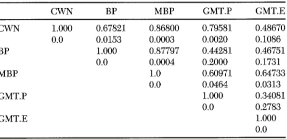
Even if these indexes include various specific factors, it is useful to see how these indexes are correlated. Table 1 presents the correlations among these different CB independence indexes. Overall, CWN provides the most general measure of CBI by including both political and economic variables. BP, MBP and GMT.P use political variables, while GMT.E uses economic variables, to construct the rankings. Standard errors are reported beneath each correlation. 9 There are positive correlations among the indexes. The strongest correlation is between BP and MBP. The reason could be that MBP is a modified version of the BP. Not surprisingly, given that these indices use different measures to construct the rankings, the weakest correlation is between GMT.P and GMT.E.

(8)

Hakan Berument

TABLE 1. Correlation among Various Central Banks" Independence Indexes~ CWN BP MBP GMT.P GMT.E CWN 1.000 0.67821 0.86800 0.79581 0.48670 0.0 0.0153 0.0003 0.0020 0.1086 BP 1.000 0.87797 0.44281 0.46751 0.0 0.0004 0.2000 0.1731 MBP 1.0 0.60971 0.64733 0.0 0.0464 0.0313 GMT.P 1.000 0.34081 0.0 0.2783 GMT.E 1.000 0.0

f Standard errors are reported under the correlations.

4. The Empirical Evidence

The first aim of this section is to test whether seigniorage revenue creation can be explained by the optimum financing model under different levels of CBI by using a pooled time series-cross section procedure. Also, the literature assumes that inflation is a proxy for seigniorage. Hence, the second aim of this section is to consider another model where the inflation is a proxy for seigniorage revenue. 1°

The CBI index is prepared as a constant number for each country across the given time period. Hence, single country regression coefficients could not be estimated when the CBI index is used as an additional variable because of perfect multicollinarity. Furthermore, performing the least square method does not incorporate any contemporaneous relations among residual and group-wise heterogeneity to improve efficiency. Hence, we estimate the testable equations by using the Parks (1967) procedure. The procedure performs the generalized least squares method (GLS) across countries and estimates the model by considering, first, any autocorrelation for 1°Various other definitions of seigniorage revenue, as described in Cukierman, Edwards and Tabellini (1992), are also used as a proxy for seigniorage and with their analog for tax revenue. The proxies for seigniorage considered were change in base-GNP ratio and change in base- government spending ratio, inflation times base-GNP ratio, inflation times base-government spending ratio, change in monetary base-price ratio. Even though these proxies for seigniorage gave parallel results with monetary base growth and inflation, the strongest positive association for the tax and seigniorage revenues was obtained when the seigaiorage revenue is proxied by monetary base growth and inflation. Hence, we report only these.

(9)

TABLE 2. 1972-1989t

Central Bank Independence The Empirical Evidence on the Optimum Financing Model:

In mt In mr-1

Dep. Var. Constant Time ln0t Yt Yt SSR

In Mt 0.4352 - 0 . 0 0 2 0.0506 0.0875 265.47

Mt-i 16.271 - 5 . 2 1 4 6.2396 11.058

In Pt 0.2438 - 0 . 0 0 1 0.0351 0.0299 268.22

Pt-i 15.887 - 3 . 5 4 2 8.5499 9.5928

NOTE: ln0t = logarithm of the tax rate; ln[mjyt] = logarithm of the real monetary base- real GNP ratio; ln[mt_l/yt] = logarithm of the lag value of the real monetary base-real GNP ratio; cbi = central bank independence index; SSR is the sum of squared residuals. SSRs are calculated after the Parks estimation, which performs the generalized least squares estimation; consequently, SSRs are close to the number of observations in the sample.

~t-ratios are reported under the corresponding estimated coefficients.

each country, second, for any group wise heterogeneity across countries, and third, for any cross-country correlation. The method also constrains the estimated coefficients for each country such that each variable has the same estimated coefficient across countries.

Before presenting the evidence for our baseline models, single country regressions, after considering for the first degree autoeorrelation, is exam- ined. We regress both money growth and inflation rates on constant term, time trend, tax rate and money-income ratio. This study does not find positive and statistically significant coefficients for the tax rates for most of the eighteen countries. This evidence is consistent with Grilli, Masciandaro and Tabellini (1991)'s single equation estimation results (to save space, the single country regression results are not reported here). Next, we estimate the same model by pooling data for eighteen countries. Positive and statistically significant coefficients of the tax rates are found that support the implication of the optimum financing model. The reason why we found stronger supporting evidence for the model could be that we used a more efficient estimation method, GLS, than the ordinary least squares method (Table 2). Furthermore, when the data set is pooled, the variability of the tax rate increases and this improves the efficiency of the estimates compared to single country regression results.

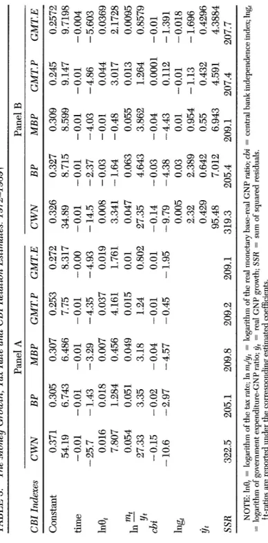
This section also considers empirical evidence for two models. The frst model is a relationship among monetary base growth, tax rate and CBI, as suggested by Equation (8). Panel A of Table 3 reports the results for the model in which the monetary base is the dependent variable. Each column reports the estimates of the model when different CBI indexes are used.

(10)

TABLE 3. The .Money Growth, Tax Rate and CBI Relation Estimates: 1972-1989~ Panel A Panel B CBI Indexes CWN BP MBP GMT.P GMT.E CWN BP MBP GMT.P GMT.E Constant 0.371 0.305 0.307 0.253 0.272 0.326 0.327 0.309 0.245 0.2572 54.19 6.743 6.486 7.75 8.317 34.89 8.715 8.599 9.147 9.7198 time - 0.01 - 0.01 - 0.01 - 0.01 - 0.00 - 0.01 - 0.01 - 0.01 - 0.01 - 0.004 - 25.7 - 1.43 - 3.29 - 4.35 - 4.93 - 14.5 - 2.37 - 4.03 - 4.86 - 5.603 ln0t 0.016 0.018 0.007 0.037 0.019 0.008 -0.03 -0.01 0.044 0.0369 7.807 1.284 0.456 4.161 1.761 3.341 - 1.64 -0.48 3.017 2.1728 In m___~t 0.054 0.051 0.049 0.015 0.01 0.047 0.063 0.055 0.013 0.0095 Yt 27.33 3.35 3.18 1.24 0.802 27.35 4.643 3.862 1.264 0.8579 cbi - 0.15 - 0.02 - 0.04 - 0.01 0.01 - 0.14 - 0.03 - 0.04 0.0001 - 0.01 - 10.6 - 2.97 - 4.57 - 0.45 - 1.95 - 9.79 - 4.38 - 4.43 0.112 - 1.391 lng t 0.005 0.03 0.01 - 0.01 - 0.018 2.32 2.389 0.954 -1.13 -1.696 Yt 0.429 0.642 0.55 0.432 0.4296 95.48 7.012 6.943 4.591 4.3884 SSR 322.5 205.1 209.8 209.2 209.1 319.3 205.4 209.1 207.4 207.7 NOTE: ln0t = logarithm of the tax rate; In mt/y t = logarithm of the real monetary base-real GNP ratio; cbi = central bank independence index; lng t = logarithm of government expenditure-GNP ratio; Yt = real GNP growth; SSR = sum of squared residuals. tt-ratios are reported under the corresponding estimated coefficients.

(11)

Central Bank Independence

Both the money growth rate and tax rates appear to have time trends. Per- forming a single regression analysis for Equation (8) may capture the time trend that both the logarithm of the tax rate and the money growth rate share. Hence, before estimating the model, the time trend is included in the regression analysis, n As the optimum financing model suggests, the estimated coefficients of the tax rate are always positive for all the estimates performed for each CBI index. Three of these five coefficients are statistically significant at least at the 10% level of confidence. The estimated coefficients for the CBI indexes are always negative, as the model suggests, and significant for four out of the five cases. 12 Hence, these results suggest that there is a positive relation between tax and seigniorage revenues and an inverse relation between creation of seigniorage revenue and the independence of the CB.

It is plausible that the positive relationship between the money growth rate and the tax rate reported in Panel A of Table 3 is proxying a relationship other than that suggested by the optimum financing model. Hence, in this study we also performed regression analyses in which other possible government concerns are considered. The first additional concern is the possi- bility governments respond to business cycles; therefore, to control this factor, a proxy for business cycles, the growth rate of real GNP, is included in the regression analysis on an ad hoc basis, is The second possible concern is whether CB's responded to changes in the interest rates which are due to government deficits. Governments do not have complete control over the interest rate; rather, the interest rate could be influenced by a changing government deficit. Increasing government spending will increase the interest rate, and the CB may increase the money supply to offset this increase. To eontrol for the second factor, a measure of government spending is also included. Therefore, both the growth of the real GNP Yt, and the logarithm of the government spending-GNP ratio, lngt, are included in the regression analysis.

Panel B of Table 3 reports the results after including those two additional variables into the model. The results do not reject the implications of either the hypothesis that there is a positive relationship between tax and

nBoth Mankiw and P&R included the time trend in their models before testing. 12The level of significance is 5% unless otherwise noted.

13Unemployment rates could be used as a proxy for business cycles. We, however, could not use it as a proxy for two reasons. First, when pooling the unemployment data several missing observations appeared for some countries. Hence, we could not create a pooled data set for eighteen OECD countries in our study using the standardized unemployment rates from OECD sources. Second, figures from a long data set available on IMF-IFS tapes could not be used as proxies for business cycles because each of the eighteen countries used different unemployment calculation methods.

(12)

Hakan Berument

seigniorage revenues or the hypothesis that higher levels of CBI is associated with lower levels of seigniorage revenue creation. However, the estimated coefficient of the tax rate is negative when the BP and MBP indexes are used. The coefficients are not significant for either ease.

Even if the results on the government spending coefficient are mixed, growth is associated with higher seigniorage revenue. The estimated coefficient for the lng t is positive when the CWN, BP and MBP indexes are used as a measure of CBI. However, this coefficient associated with the MBP index is insignificant; furthermore, the coefficient is negative and insignificant for the GMT indexes. The findings in the literature are mixed as well; Evans (1988 and 1989) shows that for the U.S., the level of government spending or the deficit does not affect private consumption, investment, nominal interest rates or inflation. The estimated coefficients for the real GNP growth are positive and statistically significant for all the CBI indexes we consider. These results may suggest that a government's monetary policies respond to the state of the economy. 14

The second model is a relationship among inflation, the tax rate and CBI; this model is derived when the seigniorage revenue is proxied by the inflation rate. Panel A of Table 4 reports the results for this analysis. The estimated coefficients of the tax rate are always positive and significant for all the CBI indexes considered. The coefficients of the CBI are negative and significant at least at the 10% level for four out of the five indexes considered. When a government's other possible concerns are included, the results are reported in Panel B. The estimated coefficients for the tax rate are found positive and significant. The CBI index has negative and significant coefficients for the CWN, BP and MBP indexes. The coefficients for the GMT indexes remained negative but statistically insignificant. The estimated coefficients for the government spending-GNP ratio and the growth rate are both negative and statistically significant. Economic reasoning behind this finding is that the government may adopt stabilizing policies to decrease inflation when it is high by reducing government spending. Therefore, this suppresses the economic growth.

Estimates reported in Tables 3 and 4 might suffer from the simulta- neous equation bias problem. The first reason is that the theory presented in Section 2 assumes that governments determine tax and seigniorage revenues simultaneously. Second, the first-order conditions not only imply that the marginal deadweight loss of taxation is equal to the marginal deadweight loss of the money growth, but also imply that the marginal deadweight loss of taxation (or money growth) must be the same across time; hence, both

14The analyses are repeated for the growth rate of the real GDP. The simdar results are found.

(13)

TABLE 4. The Inflation, Tax Rate and CBI Relation Estimates 1972-19891 Panel A Panel B CBI Indexes CWN BP MBP GMT.P GMT.E CWN BP MBP GMT.P GMT.E Constant 0.228 0.228 0.218 0.25 0.233 0.22 0.191 0.187 0.217 0.2113 26.73 11.12 14.26 12.22 10.35 56.3 11.92 15.43 12.43 9.6158 time - 0.01 - 0.01 - 0.01 - 0.01 - 0.01 - 0.01 - 0.01 - 0.01 - 0.01 - 0.003 -14.6 -4.39 -6.24 -4.58 -3.74 -32.7 -5.94 -13.7 -7.46 -9.221 ln0t 0.033 0.012 0.023 0.044 0.035 0.042 0.028 0.037 0.055 0.0565 16.81 2.003 4.012 7.686 5.839 37.14 3.857 6.363 11.54 10.332 In mt-1 0.021 0.019 0.015 0.019 0.012 0.017 0.004 0.01 0.004 2.6E-05 Yt 17.71 4.335 3.455 4.212 2.502 31.08 0.962 - 0.31 1.145 0.0082 cbi 0.01 -0.02 -0.01 -0.01 -0.01 -0.01 -0.01 -0.01 -0.01 -0.001 1.058 -11.3 -4.84 -1.96 -1.94 -2.45 -3.92 -2.47 -1.1 -0.235 lngt - 0.03 - 0.02 - 0.03 - 0.03 - 0.032 -19.1 -5.47 -6.79 -7.76 8.779 Yt - 0.4 - 0.4 - 0.43 - 0.35 - 0.372 -23.4 -13.2 -13.8 -13.1 -13.71 SSR 318.7 215.2 212.9 211.4 210.4 319.4 209.4 208.4 209.2 211.84 NOTE. ln0t = logarithm of the tax rate; In mt/yt = logarithm of the real monetary base-real GNP ratio; In m t_ 1/yt = logarithm of the lag value of the real monetary base-real GNP ratao; cbi = central bank independence index; lng t = logarithm of government expenditure-GNP ratio; 0t = real GNP growth; SSR = sum of squared residuals. }t-ratios are reported under the corresponding estimated coefficients.

(14)

Hakan Berument

the tax rate and the money growth rate are random walks. Hence, both the tax rate and the money growth rate are endogenous variables. Therefore, instrumental variables (IV, hereafter) are used to re-estimate the models. The instruments are a constant, a time trend, the CBI index, the first two lag values of each of the logarithm of tax rate, the logarithm of the government spending-GNP ratio, real GNP growth, monetary base growth (or inflation) and the logarithm of the money-income ratio. To perform the IV technique, the ordinary least squares method is used for both the first and second stage regressions.

The results are reported in Tables 5 and 6 for the money growth-tax rate and inflation-tax rate relationships, respectively. Both tables indicate that none of the implications of the basic hypothesis of the paper is rejected. Panel A of Table 5 suggests that the estimated coefficients of the tax rate is negative for three out of the five indexes used for CBI. However, none of the coefficients for the tax rate are statistically significant. Similarly, the coefficient of the CBI indexes are always negative, but statistically insignificant except for the case where the GMT.E index is used. When real GNP growth and the logarithm of government spending-GNP ratio are included, the estimated coefficients for the tax rate are always positive but statistically insignificant. The only negative and statistically significant coefficient is found for the GMT.E index. Table 6 gives the IV estimates for the inflation-tax rate relationship. Estimated coefficients for the tax rates are always positive except when the BP index is used. The estimated coefficients for the CBI are always negative. Most of the estimates are statistically significant. The estimated coefficients for the government's other possible concern variables; the real growth rate is positive for the money growth rate equation, negative for the inflation equation, and they are statistically significant for both cases. The estimated coefficients for the government spending are negative for both relationships but are statistically significant only for the inflation equation. Therefore, the sign of the coefficients obtained by the IV method are similar with the Parks method. However, the number of significant coefficients obtained from the IV method is less than that from the Parks method. Some might argue that the simultaneity bias problem is the reason that stronger supporting evidence is provided for the basic hypotheses of the paper when the Parks procedure is used than when the IV method is used. However, the reason might alternatively be that the Parks method gives more efficient estimates than the IV method.

The inflation-tax rate relationship yields more economically interpret- able results than the money growth rate-tax rate relationship. The reason for this could be that the former captures the internal dynamics of the government better. If a government desires to increase its revenues, it can increase its money growth in a very short period of time; however, increasing

(15)

TABLE5. The Money Growth, Tax Rate and CB1 Relation: Estimates with Instrumental Variables, 1972-1989+ Panel A Panel B CBI Indexes CWN BP MBP GMT. P GMT. E CWN BP MBP GMT.P GMT. E Constant 0.103 0.079 0.086 0.163 0.184 0.072 0.043 0.065 0.145 0.165 2.14 1.34 1.517 3.683 4.124 1.537 0.733 1.165 3.342 3.773 time -0.01 -0.01 -0.01 -0.01 -0.00 -0.01 -0.01 -0.01 -0.01 -0.01 - 4.09 - 4.02 - 3.76 - 4.69 - 4.71 - 3.63 - 3.82 - 3.65 - 4.41 - 4.42 ln0t 0.012 - 0.01 - 0.01 0.015 - 0.01 0.034 0.028 0.014 0.029 0.0001 0.808 - 0.33 - 0.61 1.162 - 0.65 1.404 0.856 0.505 1.284 0.009 In mt -0.04 -0.04 -0.04 -0.02 -0.03 -0.04 -0.05 -0.04 -0.02 -0.03 Yt -3.44 -2.43 -2.12 -1.92 -2.49 -3.5 -2.55 -2.23 -1.82 -2.34 cbi - 0.01 - 0.01 - 0.01 - 0.01 - 0.02 0.01 0.005 - 0.01 - 0.01 - 0.01 - 0.4 - 0.54 - 1.36 - 0.83 - 2.71 0.27 0.363 - 0.49 - 0.22 - 2.54 lngt - 0.02 - 0.02 - 0.01 - 0.01 - 0.01 - 0.9 - 0.92 - 0.69 - 0.55 - 0.4 Yt 0.807 0.784 0.703 0.635 0.624 4.36 4.068 3.51 3.568 3.54 SSR 0.007 0.005 0.005 0.005 0.005 0.006 0.005 0.005 0.005 0.004 ft-ratios are reported under the corresponding estimated coefficients. ~Instruments are constant, time trend, the CBI index, the first two lags values of each of the logarithm of tax rate, real GNP growth, the logarithm of the government spending-GNP ratio, monetary base growth (or inflation) and logarithm of the money-income ratios.

(16)

TABLE 6. Inflation, Tax Rate and CBI Relation Estimates with Instrumental Variables: 1972-1989~ g~ Panel A Panel B CBI Indexes CWN BP MBP GMT.P GMT.E CWN BP MBP GMT.P GMT.E Constant 0.21 0.188 0.166 0.22 0.224 0.226 0.19 0.17 0.236 0.24 11.52 8.447 7.566 10.88 10.61 13.6 9.248 8.742 12.76 12.46 time -0.01 -0.01 -0.01 -0.01 -0.01 -0.01 -0.01 -0.01 -0.01 -0.01 -11.3 -9.04 -10.1 -10.4 -10.2 -13 -10.9 -11.9 -12 -11.7 ln0 t 0,025 - 0.01 0.006 0.023 0.024 0.045 0.011 0.026 0.04 0.048 4.292 -0.38 -0.85 3.894 3.129 -5.047 0.905 2.569 4.167 4.72 In mr-1 -0.01 -0.01 -0.01 -0.01 -0.01 -0.01 -0.01 -0.02 -0.01 -0.01 Yt - 1.99 - 1.00 -2.15 - 1.47 - 1.57 -2.77 -2.11 -3.45 -2.33 -2.57 cbi -0.02 -0.02 -0.01 -0.01 -0.01 -0.02 -0.02 -0.01 -0.01 -0.01 -1.74 -3.81 -2.67 3.23 -1.21 -1.43 -3.34 -2.41 -3.16 -1.33 lng t - 0.02 - 0.02 - 0.02 - 0.02 - 0.03 - 3,17 - 2.24 - 3.35 - 2.46 - 3.58 Yt - 0.51 - 0.51 - 0.54 - 0.52 - 0.52 -7.51 -7.11 -7.45 -6.75 -6.58 SSR 0.001 0.001 0.001 0.001 0.001 0.001 0.001 0.001 0.001 0.001 it-ratios are reported under the corresponding estimated coefficients. ~Instruments are constant, time trend, the CBI index, the first two lags values of each of the logarithm of tax rate, real GNP growth, the logarithm of the government spending-GNP ratio, monetary base growth (or inflation) and logarithm of the money-income ratios.

(17)

Central Bank Independence

taxes may take some time because of the legislative and administrative delays. Hence, both taxes and money growth may not be increased at the same period. However, increasing monetary base accelerates inflation in the next period, and this suggests that inflation and taxes might move together.

Another reason could be that increasing seigniorage revenue may not be costly if there is economic growth. However, the cost appears as inflation if money creation exceeds the growth rate of the economy. Hence, the cost of seigniorage can be measured better with the inflation rate.

In sum, when the Parks procedure is used, the evidence mostly sup- ports the hypotheses that there is a trade-off between tax and seigniorage revenue, and this revenue decreases with higher levels of CBI. The data provides the best supporting evidence for these two hypotheses, when, first, the inflation rate is the dependent variable and, second, the economic independence of the CB is used as a measure of CBI.

5. Conclusion

This paper incorporates the effects of central bank independence in the tax-seigniorage revenue trade-off which governments face to finance their spending. The following two hypotheses are tested: first, governments use both their seigniorage revenues along with their tax revenues to finance their spending; and second, governments that are associated with more independent central banks create less seigniorage revenue. Overall, these hypotheses are supported for the various central bank independence indexes used when the seigniorage revenue is proxied by both inflation and the monetary base growth rate for eighteen OECD countries from 1972 to 1989. However, when the IV technique is used, the regressions provide weaker supporting evidence when government seigniorage revenue is proxied by monetary base growth.

These results are consistent with the relevant literature on CBI (e.g., Cukierman 1992 and Alesina and Summers 1993), which suggests that more CBI leads to less inflation. Furthermore, the paper successfully demon- strates that the CBI does influence seigniorage creation.

Received.. April 1995 Final version. October 1996

References

Alesina, Alberto. "Macroeconomics and Politics." In NBER Macroeconomics

Annual, edited by Stanley Fisher. Cambridge, Massachusetts: MIT Press,

(18)

Hakan Bernment

~ . "Politics and Business Cycles in Industrial Democracies." Economic

Policy 8 (April 1989): 55-98.

Alesina, Alberto, and Lawrence H. Summers. "Central Bank Independence and Macroeconomic Performance: Some Comparative Evidence." ]our-

hal of Money, Credit and Banking 25 (May 1993): 151-62.

Bade, R., and M. Parkin. "Central Bank Law and Monetary Policy." Manu- script, 1987.

Barro, Robert and David Gordon. "Rules, Discretion and Reputation in a Model of Monetary Policy." Journal of Monetary Economics 12 (June 1983): 101-22.

Berument, Hal(an. "Political Parties and Optimum Government Financing"

Southern Economic Journal 6] (October 1994) 510-18.

Burdekin, Richard C. K., and Thomas D. Willett. "Central Bank Reform: Federal Reserve in International Perspective." Public Budgeting and Fi-

nancial Management 3 (1991) 619-50.

Cukierman, Alex. "~¢Vhy Does the Fed Smooth Interest Rates?" In Monetary

Policy on the Fed's 75th Anniversary. Proceedings of the 14th annual

Economic Policy Conference of the Federal Reserve Bank of St. Louis• Norwell, MA: Kluwer Academic Publishers, 1990.

• Central Banks Strategy, Credibility, and Independence: Theory and

Evidence. Cambridge, Mass•: MIT Press, 1992

Cukierman, Alex, Sebastian Edwards, and Guido Tabellini. "Seigniorage and Political Instability." American Economic Review 82 (June 1992): 537-55. Cukierman, Alex, Steven Webb, and Bilin Neyapti. "The Measurement of Central Bank Independence and Its Effect on Policy Outcomes•" The

World Bank Economic Review 6 (t992): 353-98.

Evans, Paul. "Are Government Bonds Net Wealth? Evidence for the United States." Economic Inquiry 26 (October 1988): 551-66.

. "A Test of Steady State Government-Debt Neutrality." Economic

Inquiry 27 (January 1989): 39-55.

Grilli, Vittorio. "Seigniorage in Europe." In A European Central Bank?, edited by Marcello De Cecco and Alberto Gionannini. Great Britain: Cam- bridge University Press, 1989.

Grilli, V. D. Masciandaro, and G. Tabellini. "Political and Monetary Insti- tutions and Public Financial Policies in the Industrial Countries•" Eco-

nomic Policy 13 (October 1991): 341-92•

Klein, M., and M. J. M. Neumann. "Seigniorage: 'What Is It and Who Gets It?'" Weltwirtschaftliches Archly 126 (1990): 205-21.

Mankiw, N. Gregory. "The Optimal Collection of Seigniorage: Theory and Evidence." Journal of Monetary Economics 20 (September 1987): 327- 41.

(19)

Central Bank Independence

when Disturbances are Both Serially and Contemporaneously Corre-

lated."

Journal of American Statistical Association 62

(June 1967): 500-

08.

Poterba, James M., and Julio Rotemberg. "Inflation and Taxation with Op-

timizing Governments."

Journal of Money, Credit, and Banking

22 (Feb-

ruary 1990): 1-18.

Tabellini, Guido. "Money, Debt and Deficits in a Dynamic Game."

Journal

of Economics Dynamics and Control

10 (1986): 427-42.

Trehan, Bharat, and Carl E. Walsh. "Seigniorage and Tax Smoothing in the

United States, 1914-1986."

Journal of Monetary Economics 25

(January