a thesis
submitted to the department of department of physics
and the institute of engineering and science
of bilkent university
in partial fulfillment of the requirements
for the degree of
master of science
By
Can ATACA
Prof. Dr. Salim C¸ ıracı (Advisor)
I certify that I have read this thesis and that in my opinion it is fully adequate, in scope and in quality, as a thesis for the degree of Master of Science.
Prof. Dr. Atilla Er¸celebi
I certify that I have read this thesis and that in my opinion it is fully adequate, in scope and in quality, as a thesis for the degree of Master of Science.
Assoc. Prof. Dr. Ulrike Salzner
Approved for the Institute of Engineering and Science:
Prof. Dr. Mehmet B. Baray
Director of the Institute Engineering and Science
Can ATACA
M.S. in Department of Physics Supervisor: Prof. Dr. Salim C¸ ıracı
July, 2008
In this thesis we investigated structural, electronic and magnetic properties of 3d (light) transition metal (TM) atomic chains and Cr nanowires using first-principles pseudopotential plane wave calculations. Infinite periodic linear, dimer-ized linear and planar zigzag chain structures, as well as their short segments consisting of finite number of atoms and chromium nanowires have been consid-ered. For most of the infinite periodic chains, neither linear nor dimerized linear structures are favored; to lower their energy the chains undergo a structural trans-formation to form planar zigzag and dimerized zigzag geometries. Dimerization in both infinite and finite chains are much stronger than the usual Peierls distortion and appear to depend on the number of 3d -electrons. As a result of dimerization, a significant energy lowering occurs which, in turn, influences the stability and physical properties. Metallic linear chain of vanadium becomes half-metallic upon dimerization. Infinite linear chain of scandium also becomes half-metallic upon transformation to the zigzag structure. The end effects influence the geometry, energetics and the magnetic ground state of the finite chains. Structure optimiza-tion performed using noncollinear approximaoptimiza-tion indicates significant differences from the collinear approximation. Variation of the cohesive energy of infinite and finite-size chains with respect to the number of 3d -electrons are found to mimic the bulk behavior pointed out by Friedel.
Furthermore, we considered Cr nanowires, which have cross section compris-ing a few (4,5 - 9,12) atoms. Chromium nanowires are found to be in a local minimum in the Born-Oppenheimer surface and are ferrimagnetic metals. The type of coupling, as for ferromagnetic or antiferromagnetic, between neighboring Cr atoms depends on their interatomic distances. The spin-orbit coupling of finite chains are found to be negligibly small for finite molecules and Cr nanowires.
Keywords: ab initio, first principles, density functional theory, transition metal, monatomic chains, nanowires, transition metal molecules.
GEC
¸ ˙IS
¸ METAL˙I NANOTELLER˙IN MANYET˙IZMASI
Can ATACAFizik Bolumu , Y¨uksek Lisans Tez Y¨oneticisi: Prof. Dr. Salim C¸ ıracı
Temmuz, 2008
Bu tezde, 3d (hafif) ge¸ci¸s metali atom zincirlerinin ve krom (Cr) nanotellerin elek-tronik ve manyetik ¨ozelliklerini temel prensipler yalancı potansiyel d¨uzlem dalga hesaplamalarını kullanarak inceledik. Periyodik sonsuz do˘grusal, dimerle¸smi¸s do˘grusal, d¨uzlemsel do˘grusal yapılar; ge¸ci¸s elementlerinin sonlu sayısıda atomun-dan olu¸san k¨u¸c¨uk par¸cacıkları ve krom nanoteller g¨oz ¨on¨une alındı. C¸ o˘gu periy-odik sonsuz zincirler ne do˘grusal nede dimerle¸smi¸s do˘grusal yapılar enerji olarak uygun de˘gildir; zincirler enerjilerini d¨u¸s¨urmek i¸cin yapısal de˘gi¸sim ge¸cirerek zigzag veya dimerle¸smi¸s zigzag yapılarına d¨on¨u¸s¨urler. Sonlu ve sonsuz yapılarda olan dimerle¸sme alı¸sılmı¸s Peierls bozulmasından daha kuvvetlidir ve hesaplandı˘gına g¨ore 3d orbitallerindeki elekron sayısına ba˘glıdır. Dimerle¸smenin sonucu olarak, ¨onemli ¨ol¸c¨ude enerji azalması olur ve bu yapının karalılı˘gını ve fiziksel ¨ozelliklerini etkiler. Metalik do˘grusal vanadyum zincirleri dimerle¸sme sonucu yarı-metal ¨ozellikler kazanmı¸stır. Sonsuz do˘grusal skandiyum zincirleri de zigzag yapısına d¨on¨u¸serek yarı-metal ¨ozelli˘gi kazanmaktadır. U¸c etkileri sonlu zincirlerin ge-ometrisini, ba˘glanma enerjisini ve manyetik taban halini etkilemektedir. E¸s do˘grusal olmayan manyetik yakla¸sımla yapılan yapısal optimizasyonlar do˘grusal olan manyetik yakla¸sımla kayda de˘ger de˘gi¸siklikler g¨ostermektedir. Sonlu ve son-suz zincirlerinin ba˘glanma enerjilerinin 3d elektron sayıları ile de˘gi¸smeleri kristal yapısında Friedel tarafından g¨osterilmi¸s ba˘glantıya ¸cok benzemektedir.
Bu tezde 3d ge¸ci¸s metali zincirlerden ba¸ska de˘gi¸sik kesit alanlarına sahip az sayıda atomdan (4,5 - 9,12) olu¸san Cr nanotelleri de inceledik. C¸ alı¸sılan krom nanoteller Born-Oppenheimer y¨uzeyinde yerel minimumda bulunmaktadır ve fer-rimanyetik metaldir. Kom¸su Cr atomları arasındaki manyetik etkile¸sim, antifer-romanyetik veya ferantifer-romanyetik, atomlar arasındaki uzaklı˘ga ba˘glıdır. Spin-orbit etkile¸smesi sonlu zincirler ve Cr nanoteller i¸cin ¸cok k¨u¸c¨uk oldu˘gu incelenmi¸stir. Anahtar s¨ozc¨ukler: ab initio, temel prensipler, yo˘gunluk fonksiyonel teorisi, ge¸ci¸s
This thesis would not appear in its present form without the kind support of my supervisor Prof. Dr. Salim C¸ ıracı. I would like to thank him for his commitment to helping see this thesis through to its final copy and his equally generous and wise guidance during its development. I am also grateful to him for giving me a chance to complete my Master in less than ten months. I am and will be proud of working in his group all through my life.
I would like to thank to Haldun Sevin¸cli, Ethem Akt¨urk, Engin Durgun, Mehmet Topsakal, Erman Bekaro˘glu and Seymur Cahangirov for their friendship and advises.
Finally, I am forever indebted to my family for their understanding, endless patience and encouragement whenever I needed.
1 Introduction 1 1.1 3d Transition Metal Monatomic Chains and Chromium Nanowires:
Novel, Promising Nanomagnets and Spintronic Devices . . . 2
1.2 Motivation . . . 3
1.3 Organization of the Thesis . . . 4
2 Theoretical Background 5 2.1 Quantum Theory of Molecular Magnetism . . . 5
2.2 Density Functional Theory . . . 9
2.2.1 Total Energy Pseudopotential Calculations . . . 10
2.2.2 Noncollinear Magnetism . . . 18
3 3d Transition Metal Monatomic Chains 21 3.1 Method of calculations . . . 22
3.2 Infinite and Periodic Chain Structures . . . 23
3.3 Short Chain Structures . . . 35
3.3.1 Collinear Approximation . . . 35
3.3.2 Noncollinear approximation and the spin-orbit interaction 40 4 Electronic and Magnetic Properties of Cr Nanowires 46 4.1 Method of calculations . . . 47
4.2 Cr Infinite Monatomic Chain Structures . . . 48
4.3 Various size Chromium Nanowires . . . 53
4.3.1 Structure Optimization . . . 53
4.3.2 Stability and Elastic Properties . . . 59
4.3.3 Electronic and Magnetic Properties . . . 62
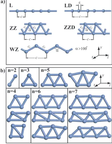
3.1 Various structures of 3d -TM atomic chains. (a) Infinite and peri-odic structures; L: The infinite linear monatomic chain of TM atom with lattice constant, c. LD: The dimerized linear monatomic chain with two TM atoms in the cell. ǫ is the displacement of the second atom from the middle of the unit cell. ZZ: The pla-nar zigzag monatomic chain with lattice parameter c and unit cell having two TM atoms. c1 ∼ c2 and 590 < α < 620. ZZD: The
dimerized zigzag structure c1 6= c2. WZ: The wide angle zigzag
structure c1 ∼ c2, but α > 1000. (b) Various chain structures
of small segments consisting of finite number (n) of TM atoms, denoted by (TM)n. . . 24
3.2 The energy versus lattice constant, c, of various chain structures in different magnetic states. FM: ferromagnetic; AFM: antiferromag-netic; NM: nonmagantiferromag-netic; FMD: ferromagnetic state in the linear or zigzag dimerized structure; AFMD: antiferromagnetic state in the dimerized linear or zigzag structure. The energy is taken as the energy per unit cell relative to the free constituent atom en-ergies in their ground state (See text for definition). In order to compare the energy of the L structure with that of the LD, the unit cell (and also lattice constant) of the former is doubled in the plot. Types of structures identified as L, LD, ZZ, ZZD, WZ are describes in Fig. 3.1. . . 27
3.3 The plot of charge accumulation, namely the positive part of the difference between the charge density of the interacting system and that of the non-interacting system, for the linear (L) and the dimerized linear structure (LD) of Cr monatomic chains. Contour spacings are equal to ∆ρ = 0.0827e/˚A3 . The outermost contour
corresponds to ∆ρ = 0.0827e/˚A3 . Dark balls indicate Cr atom. . 30
3.4 Variation of the nearest neighbor distance of 3d -TM atomic chains and the bulk structures. For the linear and zigzag structures the lowest energy configuration (i.e. symmetric or dimerized one) has been taken into account. Experimental values of the bulk nearest neighbor distances have been taken from Ref.citekittel]. . . 30 3.5 Variation of the cohesive energy, Ec (per atom), of 3d -TM
monatomic chains in their lowest energy linear, zigzag and bulk structures. For the linear and zigzag structures the highest cohe-sive energy configuration (i.e. symmetric or dimerized one) has been taken into account. Experimental values of the bulk cohesive energies have been taken from Ref.[[55]] . . . 31 3.6 Variation of the binding energy difference, ∆E (per atom) between
the lowest antiferromagnetic and ferromagnetic states of 3d -TM monatomic chains. Open squares and filled circles are for the sym-metric zigzag ZZ and dimerized zigzag ZZD chains respectively. . 31 3.7 Energy band structures of 3d -TM atomic chains in their L and
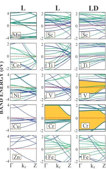
LD structures. The zero of energy is set at the Fermi level. Gray and black lines are minority and majority bands, respectively. In the antiferromagnetic state majority and minority bands coincide. Energy gaps between the valence and the conduction bands are shaded. . . 32
3.8 Energy band structures of 3d -TM atomic chains in their zigzag (ZZ) and dimerized zigzag (ZZD) structures. The zero of energy is set at the Fermi level. Gray and black lines are minority and majority spin bands, respectively. The gray and dark lines coincide in the antiferromagnetic state. Only dark lines describe the bands of nonmagnetic state. The energy gap between the valence and the conduction bands is shaded. . . 34 3.9 Variation of the average cohesive energy of small segments of chains
consisting of n atoms. (a) The linear chains; (b) the zigzag chains . In the plot, the lowest energy configurations for each case obtained by optimization from different initial conditions. . . 38 3.10 The atomic magnetic moments of some finite chains of 3d
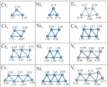
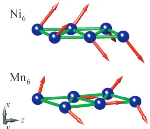
transi-tion metal atoms. Numerals on the atomic sites stand for the value of the atomic magnetic moments. Positive and negative numerals are for spin-up and spin-down polarization, respectively. Because of finite-size of the zigzag chains, the end effects are usually appear by different values of magnetic moments on atoms at the end of the chain. . . 43 3.11 Atomic magnetic moments of Ni6 and Mn6 planar zigzag chains
calculated by noncollinear approximation including sporbit in-teraction. The magnitudes and directions of magnetic moments are described by the length and direction of arrows at each atom. 44
4.1 Various structures of Cr monatomic chains. (a) Infinite and peri-odic structures; L: The infinite linear monatomic chain of Cr with lattice constant, c. LD: The dimerized linear monatomic chain with two Cr atoms in the cell. ǫ is the displacement of the sec-ond atom from the middle of the unit cell. ZZ: The planar zigzag monatomic chain with lattice parameter c and unit cell having two Cr atoms. c1 ∼ c2 and 590 < α < 620. ZZD: The dimerized zigzag
structure c1 6= c2. (b) Structures of Cr nanowires consisting of 9
and 21 atoms in a unit cell. . . 49 4.2 (a) Energy band structures of Cr monatomic chains in its L, LD,
ZZ and ZZD structures. The zero of energy is set at the Fermi level. Gray and black lines are minority and majority spin bands, respec-tively. The gray and dark lines coincide in the antiferromagnetic state. The energy gap between the valence and the conduction bands is shaded.(b) The plot of charge accumulation, namely the positive part of the difference between the charge density of the interacting system and that of the non-interacting system, for the linear (L) and the dimerized linear structure (LD) of Cr monatomic chains. Contour spacings are equal to ∆ρ = 0.0827e/˚A3 . The
outermost contour corresponds to ∆ρ = 0.0827e/˚A3 . Dark balls
indicate Cr atom. . . 52 4.3 (Upper panels) Variation of binding energy with respect to the
lattice constant for single and double cell CrNW(9) structures. Change of total magnetic moment for single cell CrNW(9) is also indicated. Distribution of interatomic distance both for single and double CrNW(9) structures are shown. (lower panel) . . . 55 4.4 Variation of binding energy with respect to the lattice constant for
single and double cell CrNW(21) structures. (upper row) Change of total magnetic moment for single cell CrNW(21) is also indi-cated. Distribution of interatomic distance both for single and double CrNW(21) structures are shown. (lower row) . . . 57
4.5 (a)Variation of total energy and total magnetic moment as the distance between two consecutive unit cell increases. (b) A sketch of the new structure with varying distance d. Plot of interatomic distances for CrNW(9) and CrNW(9) molecule. . . 61 4.6 Energy band structures of CrNW(9) structure. (a) The zero of
en-ergy is set at the Fermi level. Gray and black lines are minority and majority spin bands, respectively. Density of states for minority and majority spin bands are also included. (b) Collinear magnetic moment distribution on the atoms of CrNW(9) unit cell is given. The length and direction of arrows on each atom are proportional with the actual magnetic moments. . . 63 4.7 Energy band structures of CrNW(9) structure calculated with
non-collinear magnetic moment formalism. Spin-orbit coupling effects are also included. (a) The zero of energy is set at the Fermi level. Density of states of the system is indicated. (b) Noncollinear mag-netic moment distribution on the atoms of CrNW(9) unit cell is given. The length and direction of arrows on each atom are pro-portional with the actual magnetic moments. . . 64 4.8 Energy band structures of CrNW(21) structure. (a) The zero of
energy is set at the Fermi level. Gray and black lines are minority and majority spin bands, respectively. Density of states for mi-nority and majority spin bands are also included. (b) Collinear magnetic moment distribution on the atoms of CrNW(21) unit cell is given. The length and direction of arrows on each atom are proportional with the actual magnetic moments. . . 65
3.1 The calculated values for linear structures (L and LD). The lattice constant, c (in ˚A); the displacement of the second atom in the unit cell of dimerized linear structure, ǫ (in ˚A); cohesive energy, Ec (in
eV/atom); the magnetic ground state, MGS; and the total mag-netic moment, µ per unit cell (in Bohr magnetons, µB) obtained
within collinear approximation. . . 28 3.2 The calculated values for the planar zigzag structures (ZZ and
ZZD): The lattice constant, c (in ˚A); the first nearest neighbor, c1 (in ˚A); the second nearest neighbor, c2 (in ˚A); angle between
them, α (in degrees); the cohesive energy, Ec (in eV/atom); the
magnetic ground state, MGS; and the total magnetic moment, µ per unit cell (in Bohr magnetons, µB) obtained within collinear
approximation. . . 28 3.3 The average cohesive energy Ec (in eV/atom); the net magnetic
moment µ, (in Bohr magneton µB); magnetic ordering (MO);
LUMO-HOMO gap of majority/minority states, EG↑ and EG↓, re-spectively (in eV) for lowest energy zigzag structures. p/q indicates that the same optimized structure occurred p times starting from q different initial conditions.(See text) Results have been obtained by carrying out structure optimization within collinear approxima-tion using the ultra-soft pseudopotentials. . . 37
3.4 The highest average cohesive energy, Ec(in eV/atom); the
compo-nents (µx, µy, µz) and the magnitude of the net magnetic moment
µ (in µB); LUMO-HOMO gap EG(SO coupling excluded)/ energy
gap after spin-orbit coupling was included in x− direction / in z− direction (in eV); magnetic ordering MO; Spin-orbit coupling en-ergy △Ex
so(/△Esoz ) (in meV) under x and z initial direction of easy
axes of magnetization. p (q = 5) indicates that the same optimized structure occurred p times starting from q (= 5) different initial conditions. Results have been obtained by carrying out structure optimization calculations within noncollinear approximation using PAW potentials. Mn7 is not stable in the planar ZZ structure. For
the (x, y, z) directions see Fig. 3.1 (b). These values belong to the most energetic configuration determined by noncollinear calcula-tions including spin-orbit coupling. . . 41
4.1 The average cohesive energy Ec (in eV/atom); lattice constant c
(in ˚A); displacement of the middle atom in LD structure ǫ (in ˚A), ratio of the first nearest neighbor, c1 (in ˚A) and the second nearest
neighbor c2 (in ˚A) for ZZD structure [(c1/c2) unitless]; magnetic
ground state MGS; and the total magnetic moment, µ per unit cell (in Bohr magnetons, µB) obtained within collinear approximation. 51
4.2 The average cohesive energy Ec (in eV/atom); lattice constant for
single cell structure csc (in ˚A) and for double cell structure cdc (in
˚
A); the total magnetic moment, µ per unit cell (in Bohr magnetons, µB); spring constant k (in eV /˚A2) and the radius of the nanowire
Introduction
It is a classical convention that a magnet would preserve its magnetic properties as it is chopped down to smaller pieces. However one cannot continue chopping forever since there is an atomic limit to that. So what happens to magnetic prop-erties at the atomic and molecular level is an active research area, results of which would open new doors to manufacture several devices in several areas. At atomic level, properties of magnetic materials are results of both intrinsic properties of materials and the interactions between nanoscale molecules. Intrinsic properties may differ from ionic compounds to the bulk metals. At macroscopic level, fer-romagnetic metals like Fe, Ni, and Co has varying magnetic moments and total magnetic moment is determined by the difference of majority and minority spin states which are all indicated in a band structure of any given system. Near surfaces of magnetic particle the magnetic moment per atom can change very rapidly, hence this produces larger local magnetic moments than that of the bulk structure of the material where translational symmetry is the most effective com-ponent for determination of the ground state electronic and magnetic properties. For ionic compounds, the system is characterized by spatially localized valance electrons and thus is not affected by the distance from the surface. However, for ionic compounds, exchange interactions due to incomplete coordination shell near surface, spin configurations may become disordered and reduce the average net magnetic moment. However, this disorientation can be altered by soe processes
which gives rise to several technological applications as magnetic storage.[1] The scientific research in nanomagnetism can be framed quite concisely. The goal is to (i) create, (ii) explore, and (iii) understand new nanomagnetic materials and phenomena.
1.1
3d
Transition Metal Monatomic Chains and
Chromium Nanowires:
Novel, Promising
Nanomagnets and Spintronic Devices
Fabrication of nanoscale structures, such as quantum dots, nanowires, atomic chains and functionalized molecules have made a great impact in various fields of science and technology.[2, 3, 4, 5] Size and dimensionality have been shown to strongly affect the physical and chemical properties of matter.[6] Electrons in lower dimensionality undergo a quantization which is different from that in the bulk materials.[7, 8, 9] In nanostructures, the quantum effects, in particular the discrete nature of electronic energies with significant level spacing become pronounced.
Suspended monatomic chains being an ultimate one-dimensional (1D) nanowire have been produced and their fundamental properties have been in-vestigated both theoretically and experimentally.[9, 10, 11, 12, 13, 14, 15, 16, 17, 18, 19, 20] Ballistic electron transport[7] with quantized conductance at room temperature has been observed in metallic nanowires.[10, 16] Moreover, magnetic and transport properties become strongly dependent on the details of atomic configuration. Depending on the type and position of a foreign atom or molecule that is adsorbed on a nanostructure, dramatic changes can occur in the phys-ical properties.[4] Some experimental studies, however, aimed at producing the atomic chains on a substrate.[21] Here the substrate-chain interaction can enter as a new degree of freedom to influence the physical properties.
Unlike the metal and semiconductor atomic chains, not many theoretical stud-ies are performed on transition metal[22, 23, 24, 25] (TM) monatomic chains and nanowires. TM monatomic chains have the ability to be magnetized much eas-ier than the bulk.[26] Large exchange interactions of TM atoms in the bulk are overcome by the large electron kinetic energies, which result in a nonmagnetic ground state with large bandwidth. On the other hand, geometries which are nonmagnetic in bulk may have magnetic ground states in monatomic chains.[26] In addition, it is predicted that the quantum confinement of electrons in metallic chains should result in a magnetic ground state and even in a super paramag-netic state for some of the TM chains[27] at finite temperatures. The central issue here is the stability of the chain and the interplay between 1D geometry and the magnetic ground state.[22, 25]
1.2
Motivation
From the technological point of view, TM monatomic chains and nanowires are important in the spin dependent electronics, namely spintronics.[28] While most of the conventional electronics is based on the transport of information through charges, future generation spintronic devices will take the advantage of the elec-tron spin to double the capacity of elecelec-tronics. It has been revealed that TM atomic chains and nanowires either suspended or adsorbed on a 1D substrate, such as carbon nanotubes or Si nanowires, can exhibit high spin-polarity or half-metallic behavior relevant the for the spin-valve effect.[4] Recently, first-principles pseudopotential calculations have predicted that the finite-size segments of linear carbon chains capped by specific 3d -TM atoms display an interesting even-odd disparity depending on the number of carbon atoms.[29] For example, CoCnCo
linear chain has an antiferromagnetic ground state for even n, but the ground state changes to ferromagnetic for odd n. Even more interesting is the ferromagnetic excited state of an antiferromagnetic ground state can operate as a spin-valve when CoCnCo chain is connected to metallic electrodes from both ends.[29]
As the length of the chain decreases, finite-size effects dominate the mag-netic and electronic properties.[1, 22] When compared with the infinite case, the finite-size monatomic chains are less stable to thermal fluctuations.[30] Additional effects on the behavior of nanoparticle are their intrinsic properties and the inter-action between them.[1, 30, 31, 32] Effects of noncollinear magnetism have to be taken into account as well.[33, 34, 35] The end atoms also exhibit different behav-ior with respect to the atoms close to the middle of the structure.[36] Not only the spin dependent electronic properties of TM monatomic chains or nanowires, there are potential applications as nanomagnets in imaging and storage technolo-gies which have also been the forms of interest.
Despite all interesting physical properties of TM atomic chains and nanowires, there is not much known about their atomic and electronic structures, and mag-netic properties. In this thesis we achieved better understanding of these chain structures by performing first-principles calculations for investigation of atomic, electronic and magnetic properties.
1.3
Organization of the Thesis
The thesis is organized as follows: Chapter 2 summarizes the theoretical back-ground and approximation methods used through out the study. In Chapter 3 and 4, our studies and results about 3d transition metal monatomic chains and chromium nanowires are indicated. And finally in Chapter 5, a brief conclusion summaries the result of our studies and suggests possible future works.
Theoretical Background
2.1
Quantum Theory of Molecular Magnetism
The interaction between the localized single particle magnetic moments for the majority of these molecules can be described by Heisenberg model with isotropic (nearest neighbor) interaction and additional anisotropy term. Antiferromagnetic interaction also have a strong effect on the energy and the state of the system. As a result Heisenberg Hamiltonian will be:
H = HHeisenberg+ Hanisotropy + HZeeman (2.1)
HHeisenberg = − X u,v Juv−→s (u) · −→s (v) (2.2) Hanisotropy = − N X u=1 du(−→e (u) · −→s (u))2 (2.3) HZeeman = gµB−→B ·−→S (2.4)
Juv is a symmetric matrix containing the exchange parameters between spins
at sites u and v. J is′
−′ for antiferromagnetic coupling and′+′ for ferromagnetic
coupling. The summation is taken all over all possible sites. The anisotropy term can be simplified for the specific geometry and atoms. Zeeman term in the full Hamiltonian describes the interaction with the external magnetic field. G value,
the direction of the field can be assumed to be in z− direction which simplifies the Hamiltonian. This Hamiltonian usually cannot be solved due to the huge dimensions of the matrix. For single-spin Hamiltonian the anisotropy and the Zeeman Hamiltonians in order will be:
H = −D2Sz2− D4Sz4+ H′ (2.5)
H′ = gµ
BBxSx (2.6)
In general symmetry plays an important role in calculating eigenvectors and eigenvalues of the given Hamiltonian. The computational power decreases as the symmetry of the system increases. We have to determine the dimension of the Hamiltonian. If there is no symmetry in the system, the dimension of the Hamiltonian for a spin array of N spins with different quantum numbers will be:
dim(H) =
N
Y
u=1
(2s(u) + 1) (2.7)
To divide the Hilbert space into orthogonal subspaces H(M), the Hamiltonian must commute with Sz which results in M to be a good quantum number.
dim(H) =
+SMmax
M =−Smax
, Smax =PNu=1s(u) (2.8)
For any given M, N and s(u), the dimension of the system can be calculated as the number of the product states where Pu = mu = M The solution of this
problem after simplifications will be:
dim(H(M)) = 1 (Smax− M)! [( d dz) Smax−M N Y z=1 1 − z2s(x)+1 1 − z ]z=0 (2.9)
For the case where all of the spins are equal (s), the maximum total spin quantum number is Smax = Ns, so the result simplify to:
dim(H(M)) = f (N, 2s + 1, Smax− M)where (2.10)
f (N, µ, v) = v/µ X n=0 (−1)n N n ! N − 1 + v − nµ N − 1 ! (2.11)
The dimensions of the Hamiltonian does not change when M is either ′+′ or ′
−′. The above equation is also known as a result of de Moivre equation.
If the Hamiltonian commutes with S2 and all of the individual spins are
iden-tical to the dimensions of the orthogonal eigenspace, H(S, M) can also be deter-mined from these. Raising and lowering operator can then be defined as:
S± = S
x± iSy (2.12)
For 0 < M < Smaxone dimensional H(M) can be decomposed into orthogonal
subspaces with
H(M) = H(M, M)MS−H(M + 1) (2.13)
S−H(M + 1) =L
S≥M +1H(S, M)
It is also instructive to mention the translational symmetry found in spin rings. Defining the cyclic shift operator T defined by its action on the product basis as:
T | m1, ..., mN −1, mN >=| mN, m1, ..., mN −1 > (2.14)
zk = exp{−i
2πk
N }, k = 0, ..., N − 1, pk = 2πk/N (2.15) Here k is named as translational quantum number and pkas momentum
quan-tum number or crystal momenquan-tum. T commutes with both the Hamiltonian and the total spin. As a result of this, any Hamiltonian can be decomposed into simultaneous eigenspaces of S2, S
z and T .
If the dimension of the system is small enough, the Hamiltonian matrices can be diagonalized exactly with any analytical or numerical method. For higher dimensional systems, one has to use computational resources with some different approximations. One of the simplest methods is the projection method which depends on the multiple application of the Hamiltonian. Another method which depends on partially diagonalization of the matrix is given by Cornelius Lanc-zos. The method also uses random initial vector which is used for generating orthonormal system where representation of the operator is tridiagonal. Each iteration increases the number of both column and row of the matrix by one. With growing size of the matrix eigenvalues converge to true values of Hamilton matrix.When one wants to make calculations on linear and linear finite struc-tures, DMRG method will result in the most trustable results. Mapping a higher dimensional system to a linear one is another way of using DMRG method in higher dimensional systems. The labeling of atomic sites plays an important role because only nearest neighbor interactions are taken into account. For further information on these methods, one must refer to [37].
To finalize this section, we want to point out the evaluation of thermodynamic observables as a function of temperature T and the magnetic field B. In calcu-lations we will assume that [H, Sz] = 0 commutes with each other. The energy
dependence of eigenvalues of Sz on B is supplied from the Zeeman term. Defining
the partition function as:
Z(T, B) = tr{e−βH} =X
v
eβEv(B) (2.16)
as: M(T, B) = −1ztr{gµBSzeβH} (2.17) = −gµZB X v Mve−βEv(B) (2.18) χ(T, B) = ∂M(T, B) ∂B (2.19) = (gµB) 2 kBT { 1 Z X v Mv2e−βEv(B)− (1 z X v Mve−βEv(B))2} (2.20)
Similarly internal energy and the specific heat are calculated from the Hamil-tonian as: U(T, B) = −1ztr{He−βH} (2.21) = −Z1 X v Ev(B)e−βEv(B) (2.22) C(T, B) = ∂U(T, B) ∂B (2.23) = 1 kBT2{ 1 Z X v (Ev(B))2e−βEv(B)− ( 1 z X v Ev(B)e−βEv(B))2} (2.24)
2.2
Density Functional Theory
Nearly most of the physical properties are related with the total energy or the differences between the total energies of the system. After the invention of the Quantum Mechanic (QM) Theory, we begin to have the ability to describe the events in atomic scales. In early times, modeling and calculations in QM were so hard and lengthy that physicians, chemists, etc. prefer experiments instead of calculations. As the time passed more accurate theories have been invented and computer power increases such that ‘The boundary of feasible quantum mechan-ical calculations has shifted significantly, to the extent that it may now be more cost effective to employ quantum mechanical modeling even when experiments do offer and alternative. Physicists have developed many methods can be used to calculate a wide range of physical properties of materials, such as lattice con-stants and elastic concon-stants. These methods, which require only a specification
of the ions present (by their atomic number), are usually referred to as ab initio methods.[38]
Until now there are many different ab initio methods which can result accurate answers for tens of atom. Of all of the methods, the total-energy pseudopotential method, stands alone because of the fact that it can handle better number of atoms in calculations. The increase in the number of atoms that can be han-dled is directly due to an increase in computational efficiency of the ab initio pseudopotential method in reality, which also means that there is an increasing class of problems for which it is more cost effective to use quantum-mechanical modeling than experiments to determine the physical parameters. One can eas-ily see that the cost effectiveness of quantum-mechanical modeling methods over physical experimentation will continue to increase with time.
2.2.1
Total Energy Pseudopotential Calculations
2.2.1.1 Overview of Approximations
To determine the various electronic and geometric structure of a solid requires calculations of QM total energy of the system and subsequent minimization of that energy with respect to electronic and nuclear coordinates. Because of the large mass differences between the nucleus and electrons, electrons will respond to the same forces much faster than the nucleus. We can treat nuclei adiabatically meaning that we separate the nuclear and electronic coordinates in the many-body wave function. This is also known as “Born-Oppenheimer approximation”. The total energy calculations then include density functional theory to model the electron-electron interaction, pseudopotential theory to model the electron-ion interactions, supercells to model systems with periodic geometries and iterative minimization techniques to relax the electronic coordinates.
2.2.1.2 Electron-Electron Interaction
In DFT we assume that instead of solving strongly interacting electron gas, we modeled it as a single particle moving in an effective nonlocal potential. In many electron system, the wave function has to be antisymmetric under the exchange of any two electrons because electrons are fermions. Having the wave function antisymmetric results in spatial separation between electrons that have the same spin and as a result reduces the Coulomb energy of the electronic system. This process which reduces the total energy is known as exchange energy. If electrons that have opposite spins are also spatially separated, the Coulomb energy of the total system can also be reduced below its Hartree-Fock value. The Coulomb energy of the system is reduced, but the kinetic energy of electrons did increased. The difference in energy between the results obtained from Hartree-Fock approxi-mation and the many-body energy of an electronic system is known as correlation energy.
Density Functional Theory is developed by Hohenberg, Kohn and Kohn, Sham for describing the effects of exchange and correlation in an electron gas. Hohen-berg and Kohn showed that total energy of an electron gas can be modeled as a unique functional of electron density. Kohn and Sham then showed how to represent the many-electron problem by exactly equivalent set of self consistent one-electron equations.
The Kohn-Sham energy functional for a set of doubly occupied electronic states is given as:
E[ψi] = 2 X i Z [−¯h 2 2m]∇ 2ψ id3r + Z Vion(r)n(r)d3r + (2.25) e2 2 Z n(r)n(r′ ) | r − r′ |d 3rd3r′ + EXC[n(r)] + Eion(RI)
Eion is the Coulomb energy provided with interactions among the ions
(nu-cleus) at position RI, Vion is the total electron-ion potential, n(r) is the electron
n(r) = 2X
i
| ψi(r) |2 (2.26)
Determining the set of wave functions ψi that gives minimum Kohn-Sham
energy functional: {−¯h 2 2m ▽ 2+V ion(r) + VH(r) + VXC(r)}ψi(r) = ǫiψi(r) (2.27)
Here ψirepresents the wave function of the ithelectronic state and ǫi represents
the corresponding eigenvalue. VH(r) is the Hartree potential and VXC(r) is the
exchange correlation potential.
VH(r) = e2 Z n(r′ | r − r′ |d 3r′ (2.28) VXC(r) = δEXC[n(r)] δn(r) (2.29)
These equations represent a mapping of the interacting many-electron sys-tem to a syssys-tem of noninteracting electrons in an effective potential caused by all other electrons. We must solve these equations self consistently because the occu-pied electronic states generate a charge density which will produce the electronic potential which are used in constructing these equations. The Kohn-Sham eigen-values are not the energies of the single particle electron states, but rather the derivatives of the total energy with respect to the occupation numbers of these states. Nevertheless, the highest occupied eigenvalue in an atomic or molecular calculation is nearly the unrelaxed ionization energy for that system.[39]
The universally used and easiest method used for describing the exchange-correlation energy of an electronic system is local-density approximation (LDA). The main idea behind this approximation is that the exchange-correlation energy of an electronic system is constructed by assuming that the exchange-correlation
energy per electron at a point r n the electron gas, ǫXC(r), is equal to the
exchange-correlation energy per electron in a homogeneous electron gas that has the same density as the electron at point r.
EXC[n(r)] = Z ǫXC(r)n(r)d3r (2.30) δEXC[n(r)] δn(r) = δ[n(r)ǫXC(r)] δn(r) (2.31) ǫXC(r) = ǫhomXC [n(r)] (2.32)
LDA ignores corrections to the exchange-correlation energy at a point r due to nearby inhomogeneities in the electron density. Shortly we can conclude that LDA appears to give a single well-defined global minimum for the energy of a non-spin-polarized system of electrons in a fixed ionic potential. For magnetic material, one has to expect more than one local minimum in energy. The global minimum of the system is then found by monitoring energy functional over a large region of phase space.
2.2.1.3 Periodic Supercells
Up to now I mentioned DFT on small number of atoms. When the system is periodic there are infinitely many number of atoms and electrons. As a result we must include all of the interactions of these particles in our calculations. There are two difficulties of this result. Wave functions must be calculated for each of the infinitely many electrons in the system and the basis set required to expand each wave function is infinite. Here we will use Bloch’s Theorem to make life easier.
This theorem states that in a periodic solid each electron wave function can be written as the product of a cell-periodic part and a wavelike part:
Periodic part of the wave function can be expanded using a basis set consisting of a discrete set of plane waves :
fi(r) =
X
G
ci,Gexp[iG · r] (2.34)
Here reciprocal lattice vectors G are defined by using the fact that G.l = 2πm. Here l is a lattice vector and m is an integer. Then wave function for each electron can be written as :
ψi(r) =
X
G
ci,k+Gexp[i(k + G) · r] (2.35)
By using the boundary conditions electronic states are allowed only at a set of k points in a bulk solid. There is a direct proportionality between the volume of the solid in reciprocal space and the density of allowed k points. By using the Bloch’s Theorem we change the problem of calculating infinite number of electronic wave functions to the one of calculating a finite number of electronic wave functions at an infinite number of k points. The electronic wave functions at k points that are very close together will be almost identical and hence it is possible to represent the electronic wave functions over a region of k space by the wave functions at a single k point. In this case the electronic states at only a finite number of k points are required to calculate the electronic potential and hence determine the total energy of the solid. The electronic potential and total energy are more difficult to calculate if the system is metallic because a dense set of k points is required to define the Fermi surface precisely. The magnitude of any error in the total energy due to inadequacy of the k point sampling can always be reduced by using a denser set of k points. The computed total energy will converge as the density of k points increases.[40]
We know that we can expand electronic wave functions at each k point any discrete plane wave basis set by Bloch’s Theorem. The coefficients ci,k+G for the
plane waves with small kinetic energy are typically more important those with having a larger energy. By this way we can truncate the plane-wave basis set to include only plane waves that have kinetic energies less than some cutoff energy. Introduction of this cutoff energy to the discrete plane-wave basis set produces a finite basis set. The energy cutoff will lead to small error in total energy calculations, but increasing the value of the cutoff energy, the total energy will converge to a value. By using a denser k point sets we can overcome the problem of discontinuities occurred at different cutoffs for different k points in the k-points set.
Plane-wave representation of Kohn-Sham equations are : X G′ [¯h 2 2m | k + G | 2 δ GG′ + Vion(G − G′) + (2.36) VH(G − G′) + VXC(G − G′)]ci,k+G′ = ǫici,k+G
The kinetic energy of electrons is diagonal, and the many potentials are described in terms of their Fourier transforms. The dimension of the matrix depends on the cutoff energy value we choose.
2.2.1.4 Electron-Ion Interactions
To perform calculation including the effect of all ions and electrons, an extremely large plane wave basis set would be required and a huge amount of computational time would be required to calculate the electronic wave function. It is well known that most physical properties of solids are dependent on the valance electrons to a much greater extent than the core electrons. The pseudopotential approxima-tion exploits this by removing the core electrons and by replacing them and the strong ionic potential by a weaker pseudopotential that acts on a set of pseudo wave functions rather than the true valance wave function. The valance wave functions oscillate rapidly in the region occupied by the core electrons due to the strong ionic potential in this region. These oscillations maintain the orthog-onality between the core wave functions and the valance wave functions, which is required by the exclusion principle. The scattering from the pseudopotential
must be angular momentum dependent because the phase shift introduced by the ion core is different for each angular momentum component of the valance wave function.
VN L =
X
lm
| lmiVlhlm | (2.37)
Here | lm > represents the spherical harmonics and Vl is the pseudopotential
for the angular momentum. A local pseudopotential uses the same potential for all the angular momentum components and its amplitude is only a function of the distance from the nucleus.
We refer to the electron density in the exchange-correlation energy in total energy calculations. If we can find the accurate exchange-correlation energy, we must have the pseudo and real wave function to be identical in both amplitude and spatial dependences. These will result in charge densities to be the same. Nonlocal pseudopotential that uses different potential for different angular mo-mentum values will describe the scattering from the ion core the best. The one to one correspondence between the pseudo and real wave functions outside the core region also proves that the first order energy dependence of the scattering from the ion core is correct, which results in scattering process is accurately described over a wide range of energy.
As we use pseudopotential in our calculation we can use fewer plane wave basis states. By this way we removed the rapid oscillations of the valance wave function in the core region of the atom. Small core region electrons are not present at this time. The total energy of the system is much less than the case of all-electrons, but the difference between the electronic energies of different ionic configurations is very similar to all electron case. We can conclude that the total energy is meaningless until now. The true and the important value are the differences in energies.
2.2.1.5 Ion-Ion Interaction
The Coulomb interaction in real and reciprocal space is long ranged. We have to develop another method for including effects of ion-ion interactions. Using Edwald’s method, one can obtain the equation given below.
X l 1 R1+ l − R2 = √2 2π X l Z ∞ η exp[− | R 1 + l − R2 |2 ρ2]dρ + (2.38) 2π Ω X G Z η 0 exp{− | G |2 4ρ2 }xexp[i(R1− R2) · G] 1 ρ3dρ
Where l is lattice vectors ad G is reciprocal lattice vectors and Ω is the volume of the unit cell as before. In this method we try to write the lattice summation of the Coulomb energy with respect to the interaction between an ion positioned at R2 and an array of atoms positioned at R2+ l. This valid for ‘+′ values of the
variable η. If we can find an appropriate value for this variable, two summations became rapidly convergent. As a result real and reciprocal space summation can be calculated by few lattice vectors and few reciprocal vectors. For the calculation of the correct energy, we must remove G = 0 contribution of the Coulomb energy of the ionic system. Omitting G = 0 summation in reciprocal space finally we achieve the relation as :
Eion = 1 2 X I,J ZIZJe2{ X l erf c(η | R1+ l − R2 |) | R1+ l − R2 | − 2η √ 2ρδIJ + (2.39) 4π Ω X G6=0 1 | G |2exp{− | G |2 4η2 }cos[(R1− R2) · G] − π η2Ω}
Z is the valances of ions I and J.erf c is the error function. L = 0 term is neglected because ion does not interfere with its own charge.
2.2.2
Noncollinear Magnetism
In cases where both AFM and FM couplings occur and compete with each other, collinear magnetism fails for modeling the ground state magnetic ordering. A midway between AFM and FM exchange interactions results in allowing the spin quantization axis to vary in every site of the structure. Geometric structure also influences noncollinear magnetism. Frustrated antiferromagnets having tri-angular lattice structure, disordered systems as well as broken symmetry on the surface will result in noncollinear magnetism. Spin glasses, α-Mn, domain walls, Fe clusters are typical examples of noncollinearity.
There are many different approaches for implementing noncollinear mag-netism, such as ASW (Augmented Spherical Wave), CPA (Coherent-Potential Approximation), LSDA (Local-Spin-Density Approximation). In our study, we use fully unconstrained approach to noncollinear magnetism.[41] In the PAW method the wavefunctions ψα
n are derived from the pseudo-wavefunction fψnα by a
linear transformation in which the spin indices are included.
| ψnα >=| fψαn > +
X
i
(| φi > − | eφi >) < epi | fψnα > (2.40)
Index i is used for the atomic site R, L = l, m is the angular moment quan-tum numbers and k is referring to the reference energy ǫkl. For noncollinear
mag-netism, pseudo-wave functions are defined to consist of 2N eigenspinors where N is the total number of atoms. Pseudo-wave functions are expended in reciprocal space into plane waves
< r | fψα n >= 1 Ω1/2r X k Cnkα (r)eik/cdotr (2.41)
Where Ωr is the Wigner-Seitz cell. Partial waves φi are taken from
partial waves outside a core radius rl
c. One can obtain the AE total density matrix
starting from 2.40 and is given in 2.42
nαβ(r) = enαβ(r) +1nαβ(r) −1enαβ(r) (2.42)
where ˜n is the soft pseudodensity matrix calculated directly from the pseudo-wave functions on a plane-pseudo-wave grid. The on-site density matrices1n and 1en are
treated on a radial support grid around each atom. For detailed information on these, see [41].
The total energy functional consists of 3 terms. E = ˜E + E1− ˜E1. ˜E is the
smooth part which is evaluated on regular grids in Fourier or real space. E1 and
˜
E1 are two one-center contributions and indicated in 2.43
e E =X α X n fn < fψαn | − 1 2∆ | fψ α n > +EXC[˜nαβ+ ˆnαβ+ ˜nc] + (2.43) EH[˜nT r + ˆnT r] + Z vH[˜nZc](r)[˜nT r(r) + ˆnT r(r)]dr + U(R, Zion) ˜ E1 =X αβ X i,j ραβij < ˜φi | − 1 2∆ | ˜φj + EXC[ 1n˜αβ + ˆnαβ + ˜n c] + (2.44) EH[1˜nT r+ ˆnT r] + Z Ωr vH[˜nZc](r)[1n˜T r(r) + ˆnT r(r)]dr E1 =X αβ X i,j ραβij < φi | − 1 2∆ | φj+ EXC[ 1nαβ + n c] + EH[1nT r] (2.45) + Z Ωr vH[nZc](r)1nT r(r)dr
where U(R, Zion) is the electrostatic energy of point charges Zion in a uniform
that is equivalent to nZc inside the core region.The Hamiltonian of the system
after making simplifications and approximations will be:
Hαβ[n, {R}] = −1 2δαβ+ ˜v αβ eff + (2.46) X (i,j) | ˜pi > ( ˆDijαβ + 1Dαβ ij − 1D˜αβ ij ) < ˜pj|
Here ˜vαβeff is the effective one-electron potential which depends on the electron density and the magnetization at each site; −1
2δαβ stands for the kinetic energy of
the system. ˆDαβij , 1Dαβ
ij and 1D˜ αβ
ij terms in the summation sign over augmented
channels represent the correction terms for long range, effective potential and wave functions. For further details see Ref.[41, 42, 43, 44, 45, 46]
3d
Transition Metal Monatomic
Chains
Nowadays size is a significant criterion. Atomic scale storage devices, spin based communication and computation devices, magnetism in linear metallic structures are all a topic of intense interest in today’s world. Quantum confinement of the electrons in one or more dimension is a consequence of reducing dimensionality and size of devices. The simplest case is one dimensional transition metal mag-netic systems, which foresees a wide range of magmag-netic phenomena and properties unknown in higher dimensions. Even the fabrication of such structures is chal-lenging, the theoretical explanation is more complicated than the simple crystal structures of these systems.
In this chapter, we consider infinite, periodic chains of 3d -TM atoms having linear and planar zigzag structures and their short segments consisting of finite number of atoms. For the sake of comparison, Cu and Zn chains are also included in our study. All the chain structures discussed in this paper do not correspond to the global minimum, but may belong to a local minimum. The infinite and periodic geometry is of academic interest and can also be representative for very long monatomic chains. The main interest is, however, in the short segments comprising finite number of TM atoms. We examined the variation of energy as
a function of the lattice constant in different magnetic states, and determined stable infinite and also finite-size chain structures. We investigated the electronic and magnetic properties of these structures. Present study revealed a number of properties of fundamental and technological interest: The linear geometry of the infinite, periodic chain is not stable for most of the 3d -TM atoms. Even in linear geometry, atoms are dimerized to lower the energy of the chain. We found that infinite linear vanadium chains are metallic, but become half-metallic upon dimerization. The planar zigzag chains are more energetic and correspond to a local minimum. For specific TM chains, the energy can further be lowered through dimer formation within planar zigzag geometry. Dramatic changes in the electronic properties occur as a result of dimerization. The magnetic properties of short monatomic chains have been investigated using both collinear and non-collinear approximation, which are resulted in different net magnetic moment for specific chains. Spin-orbit coupling which is calculated for different initial easy axis of magnetization has been found to be negligibly small.
3.1
Method of calculations
We have performed first-principles plane wave calculations[38, 47] within Density-Functional Theory (DFT)[48] using ultra-soft pseudopotentials.[49] We also used PAW[50] potentials for the noncollinear and noncollinear spin-orbit calculations of the finite chains. The exchange-correlation potential has been approximated by generalized gradient approximation (GGA).[51] For the partial occupancies, we have used the Methfessel-Paxton smearing method.[52] The width of smearing for the infinite structures has been chosen as 0.1 eV for geometry relaxations and as 0.01 eV for the accurate energy band and the density of state (DOS) calculations. As for the finite structures, the width of smearing is taken as 0.01 eV. We treated the chain structures by supercell geometry (with lattice parameters asc, bsc, and
csc) using the periodic boundary conditions. A large spacing (∼ 10 ˚A) between
the adjacent chains has been assured to prevent interactions between them. In single cell calculations of the infinite systems, csc has been taken to be equal to
Bloch functions and k-points used in sampling the Brillouin zone (BZ) have been determined by a series of convergence tests. Accordingly, in the self-consistent potential and the total energy calculations the BZ has been sampled by (1x1x41) mesh points in k-space within Monkhorst-Pack scheme. [40] A plane-wave basis set with the kinetic energy cutoff ¯h2|k + G|2/2m = 350 eV has been used. In
calculations involving PAW potentials, kinetic energy cutoff is taken as 400 eV . All the atomic positions and lattice constants (csc) have been optimized by using
the conjugate gradient method where the total energy and the atomic forces are minimized. The convergence is achieved when the difference of the total energies of last two consecutive steps is less than 10−5 eV and the maximum
force allowed on each atom is 0.05 eV/˚A. As for the finite structures, supercell has been constructed in order to assure ∼ 10 ˚Adistance between the atoms of adjacent finite chain in all directions and BZ is sampled only at the Γ-point. The other parameters of the calculations have been kept the same. The total energy of the optimized structure (ET) relative to free atom energies is negative, if it is
in a binding state. As a rule, the structure becomes more energetic (or stable) as its total energy is lowered. Figure 3.1 describes various chain structures of TM atoms treated in this study. These are the infinite periodic chains and the segments of a small number of atoms forming a string or a planar zigzag geometry. The stability of structure-optimized finite chains are further tested by displacing atoms from their equilibrium positions in the plane and subsequently reoptimizing the structure. Finite-size clusters of TM atoms are beyond the scope of this thesis.
3.2
Infinite and Periodic Chain Structures
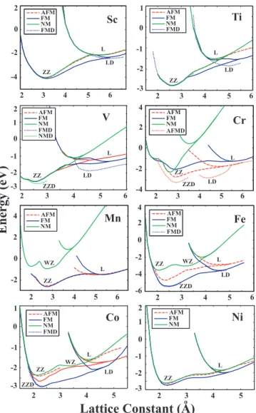
Figure 3.2 shows the energy versus lattice constant of various infinite and peri-odic chain structures (described in Fig. 3.1) in different magnetic states. These are the infinite linear (L), the dimerized linear (LD), the planar zigzag (ZZ), and the dimerized zigzag (ZZD) monatomic chains. WZ is a planar zigzag monatomic chain which has apical angle α > 1000. In calculating the ferromagnetic (FM)
state, the structure is optimized each time using a spin-polarized GGA calcula-tions starting with a different preset magnetic moment in agreement with Hund’s
n=2 n=3 n=5 n=4 n=6 n=7 c c c c c L LD ZZ ZZD WZ ε c1 c2 c1 c2 c1 c2 α α >100o z a) b) x y α α z x y
Figure 3.1: Various structures of 3d -TM atomic chains. (a) Infinite and periodic structures; L: The infinite linear monatomic chain of TM atom with lattice con-stant, c. LD: The dimerized linear monatomic chain with two TM atoms in the cell. ǫ is the displacement of the second atom from the middle of the unit cell. ZZ: The planar zigzag monatomic chain with lattice parameter c and unit cell having two TM atoms. c1 ∼ c2 and 590 < α < 620. ZZD: The dimerized zigzag
structure c1 6= c2. WZ: The wide angle zigzag structure c1 ∼ c2, but α > 1000.
(b) Various chain structures of small segments consisting of finite number (n) of TM atoms, denoted by (TM)n.
rule. The relaxed magnetic moment yielding to the lowest total energy has been taken as the FM state of the chain. For the antiferromagnetic (AFM) state, we assigned different initial spins of opposite directions to adjacent atoms and re-laxed the structure. We performed spin-unpolarized GGA calculations for the nonmagnetic (NM) state. The energy per unit cell relative to the free constituent atoms is calculated from the expression, E = [NEa − ET], in terms of the
to-tal energy per unit cell of the given chain structure for a given magnetic state (ET) and the ground state energy of the free constituent TM atom, Ea. N is
the number of TM atom in the unit cell, that is N=1 for L, but N=2 for LD, ZZ, and ZZD structures. The minimum of E is the binding energy. By conven-tion Eb < 0 corresponds to a binding structure, but not necessary to a stable
structure. The cohesive energy per atom is Ec = −Eb/N. Light transition metal
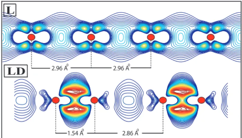
atoms can have different structural and magnetic states depending on the number of their 3d electrons. For example, Sc having a single 3d electron, has a shallow minimum corresponding to a dimerized linear chain structure in the FM state. If the L structure is dimerized to make a LD structure, the energy of the chain is slightly lowered. Other linear structures, such as linear NM, and AFM states have higher energy. More stable structure ZZ is, however, in the FM state. This situation is rather different for other 3d TM elements. For example, Cr has LD and more energetic ZZD structures in the AFM state. It should be noted that in the dimerized linear chain structure of Cr the displacement of the second atom from the middle of the unit cell, ǫ, is rather large. Apparently, the dimerization is stronger than the usual Peierls distortion. As a result, the nearest neighbor distance, (c − ǫ), is much smaller than the second nearest neighbor distance, (c + ǫ). This situation poses the question whether the interaction between the adjacent dimers are strong enough to maintain the coherence of the chain struc-ture. We address this question by comparing the energies of individual dimers with the chain structure. The formation of the LD structure is energetically more favorable with respect to individual dimer by 0.54 eV per atom. Furthermore, the charge accumulation, namely the positive part of the difference between the charge density of the interacting system and that of the non-interacting system, presented in Fig. 3.3, indicates a significant bonding between the adjacent dimers. On the other hand the bonding in a dimer is much stronger than the one in a L
chain. Nevertheless, the LD structure has to transform to more energetic ZZD structure. The zigzag structures in the AFM, FM and NM states have minima at higher binding energies and hence are unstable.
The linear structures of Ti atoms always prefer dimerized geometries and the displacement of the second atom from the middle of the unit cell is large. There is also a remarkable energy difference between L and LD structures in favor of the latter. Energies of LD AFM, FM and NM structures are very close to each other. Looking at the bandstructure of L and LD Ti chain on Fig. 3.7, it can easily be seen that dimerization forms flat bands which are results of localized electrons. This band structure suggests that Ti atoms form two atom molecules which interact weakly with adjacent dimer molecules. However, more energetic ZZ structures do not dimerize. All magnetic structures of V prefer to dimerize. Dimerization of V atoms also influence the magnetic and the electronic properties of the structure. One sees that the number of flat bands increases after dimerization. Vanadium is the only light TM monatomic ZZ chain which appears in the NM lowest energy state. The linear and the linear dimerized Fe chains have a local minimum in the FM state. More stable ZZ and ZZD structures in the FM state have almost identical minima in lower binding energy. The ferromagnetic planar zigzag chain structure appears to be the lowest energy structure for Mn. Both Co and Ni monatomic chains prefer the FM state in both L and ZZ structures. The energy of ZZ chain in the FM state is lowered slightly upon dimerization. The displacement of the second atom in ZZD structure is also not very large. It is also saliency to note that Fe, Mn and Co chains in the NM state undergo a structural transformation from ZZ to WZ structure. As the number of electrons in the d-shell of atom increases, the effect of dimerization on the energy and the geometry of the structure decreases. Therefore it can be concluded that 3d-TM atoms having fewer electrons can make hybridization easier. It is noted from Fig. 3.2 that the structure of 3d -TM atomic chains are strongly dependent on their magnetic state. Optimized structural parameters, cohesive energy, magnetic state and net magnetic moment of infinite linear and zigzag structures are presented in Table 4.1 and Table 4.2, respectively.
AFM FM NM 2 3 4 5 6 2 0 -2 -4 FMD 4 2 0 -2 -4 2 3 4 5 6 AFM FM NM AFMD -6 -4 -2 0 2 4 2 3 4 5 6 AFM FM NM FMD 2 3 4 5 6 -2 0 2 4 AFM FM NM Sc Cr Fe Mn
Lattice Constant (A)o
Energy (eV) ZZ L LD ZZ L LD ZZD WZ ZZ L LD ZZD ZZ L WZ Co AFM FM NM FMD ZZ L LD ZZD WZ 2 3 4 5 1 0 -3 -1 -2 AFM FM NM 2 3 4 5 1 0 -3 -1 -2 2 Ni ZZ L 1 0 -3 -1 -2 Ti AFM FM NM FMD 2 3 4 5 6 ZZ L LD 1 0 -1 -2 2 -3 2 3 4 5 6 AFM FM NM NMD FMD V ZZ L LD ZZD
Figure 3.2: The energy versus lattice constant, c, of various chain structures in different magnetic states. FM: ferromagnetic; AFM: antiferromagnetic; NM: non-magnetic; FMD: ferromagnetic state in the linear or zigzag dimerized structure; AFMD: antiferromagnetic state in the dimerized linear or zigzag structure. The energy is taken as the energy per unit cell relative to the free constituent atom energies in their ground state (See text for definition). In order to compare the energy of the L structure with that of the LD, the unit cell (and also lattice constant) of the former is doubled in the plot. Types of structures identified as L, LD, ZZ, ZZD, WZ are describes in Fig. 3.1.
Sc Ti V Cr Mn Fe Co Ni Cu Zn c 6.0 4.9 4.5 4.4 2.6 4.6 2.1 2.2 2.3 2.6 ε 0.38 0.52 0.51 0.66 0.0 0.21 0.0 0.0 0.0 0.0 Ec 1.20 1.83 1.86 1.40 0.76 1.81 2.10 1.99 1.54 0.15 MGS FM FM FM AFM AFM FM FM FM NM NM µ 1.74 0.45 1.00 ±1.95 ±4.40 3.32 2.18 1.14 0.0 0.0 Table 3.1: The calculated values for linear structures (L and LD). The lattice constant, c (in ˚A); the displacement of the second atom in the unit cell of dimer-ized linear structure, ǫ (in ˚A); cohesive energy, Ec (in eV/atom); the magnetic
ground state, MGS; and the total magnetic moment, µ per unit cell (in Bohr magnetons, µB) obtained within collinear approximation.
Sc Ti V Cr Mn Fe Co Ni Cu Zn c 3.17 2.60 2.60 2.90 2.76 2.40 2.30 2.30 2.40 2.50 c1 2.94 2.43 1.84 1.57 2.64 2.24 2.23 2.33 2.39 2.67 c2 2.94 2.45 2.42 2.65 2.64 2.42 2.39 2.33 2.39 2.67 α 65.2 64.5 73.8 82.6 63.0 61.9 59.6 59.1 60.2 55.8 Ec 2.05 2.78 2.64 1.57 1.32 2.69 2.91 2.74 2.16 0.37 MGS FM FM NM AFM FM FM FM FM NM NM µ 0.99 0.18 0.0 ±1.82 4.36 3.19 2.05 0.92 0.0 0.0 Table 3.2: The calculated values for the planar zigzag structures (ZZ and ZZD): The lattice constant, c (in ˚A); the first nearest neighbor, c1 (in ˚A); the second
nearest neighbor, c2 (in ˚A); angle between them, α (in degrees); the cohesive
energy, Ec (in eV/atom); the magnetic ground state, MGS; and the total
mag-netic moment, µ per unit cell (in Bohr magnetons, µB) obtained within collinear
average cohesive energy of the linear and zigzag chain structures with those of the bulk metals and plot their variations with respect to their number of 3d electrons of the TM atom. The nearest neighbor distance in the linear and zigzag structures are smaller than that of the corresponding bulk structure, but display the similar trend. Namely, it is large for Sc having a single 3d electron and decreases as the number of 3d electrons, i.e. Nd, increases to four. Mn is an
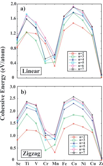
exception, since the bulk and the chain structure show opposite behavior. While the nearest neighbor distance of bulk Mn is a minimum, it attains a maximum value in the chain structure. Owing to their smaller coordination number, chain structures have smaller cohesive energy as compared to the bulk crystals as shown in Fig. 3.5. However, both L (or LD if it has a lower energy) and ZZ (or ZZD if it has a lower energy) also show the well-known double hump behavior which is characteristics of the bulk TM crystals. Earlier, this behavior was explained for the bulk TM crystals.[5, 53, 54] The cohesive energy of zigzag structures are generally ∼ 0.7 eV larger than that of the linear structures. However, it is 1-2 eV smaller than that of the bulk crystal. This implies that stable chain structures treated in this study correspond only to a local minima in the Born-Oppenheimer surface.
We note that spin-polarized calculations are carried out under collinear ap-proximation. It is observed that all chain structures presented in Table 4.1 and Table 4.2 have magnetic state if Nd< 9. Only Cr and Mn linear chain structures
and Cr zigzag chain structure have an AFM lowest energy state. The binding energy difference between the AFM state and the FM state, ∆E = EAF M
b −EbF M,
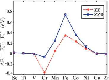
is calculated for all 3d TMs. Variation of ∆E with Nd is plotted in Fig. 3.6. We
see that only Cr ZZ and ZZD chains have an AFM lowest energy state. ∆E of Fe is positive and has the largest value among all 3d -TM zigzag chains. Note that ∆E increases significantly as a result of dimerization.
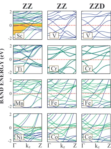
Having discussed the atomic structure of 3d -TM chains, we next examine their electronic band structure. In Fig. 3.7, the chain structures in the first column do not dimerize. The linear chains placed in the third column are dimerized and changed from the L structure placed in the second column to form the LD struc-ture. Most of the linear structures in Fig. 3.7 display a FM metallic character with
L
LD 2.96 Ao 2.96 Ao
2.86 Ao 1.54 Ao
Figure 3.3: The plot of charge accumulation, namely the positive part of the difference between the charge density of the interacting system and that of the non-interacting system, for the linear (L) and the dimerized linear structure (LD) of Cr monatomic chains. Contour spacings are equal to ∆ρ = 0.0827e/˚A3 . The
outermost contour corresponds to ∆ρ = 0.0827e/˚A3 . Dark balls indicate Cr
atom. 1 2 3 Sc Ti V Cr Mn Fe Co Ni Cu Zn Bulk (Exp.) ZZ or ZZD L or LD Bulk (Calc.)
Nearest Neighbor Distance (A)
o
Figure 3.4: Variation of the nearest neighbor distance of 3d -TM atomic chains and the bulk structures. For the linear and zigzag structures the lowest energy configuration (i.e. symmetric or dimerized one) has been taken into account. Experimental values of the bulk nearest neighbor distances have been taken from Ref.citekittel].
0 1 2 3 4 5 6 Bulk (Exp.) ZZ L Sc Ti V Cr Mn Fe Co Ni Cu Zn Bulk (Calc.)
Cohesive Energy (eV/atom)
Figure 3.5: Variation of the cohesive energy, Ec (per atom), of 3d -TM monatomic
chains in their lowest energy linear, zigzag and bulk structures. For the linear and zigzag structures the highest cohesive energy configuration (i.e. symmetric or dimerized one) has been taken into account. Experimental values of the bulk cohesive energies have been taken from Ref.[[55]]
Sc Ti V Cr Mn Fe Co Ni Cu Zn
∆
E =
Ε − Ε (
eV)
AFM FM 0 0.2 0.4 0.6 0.8 0.2 0.4 -ZZ ZZD b bFigure 3.6: Variation of the binding energy difference, ∆E (per atom) between the lowest antiferromagnetic and ferromagnetic states of 3d -TM monatomic chains. Open squares and filled circles are for the symmetric zigzag ZZ and dimerized zigzag ZZD chains respectively.
BAND ENERGY (eV) Γ kz Z Γ kz Z Γ kz Z Mn V Cr Fe Co Cu Ti Sc Ni Zn Fe Ti Sc 4 0 -4 2 0 -2 4 0 -4 4 0 -4 4 0 -4 2 0 -2 2 0 -2 2 0 -2 2 0 -2 2 0 -2 2 0 -2 2 0 -2 2 0 -2 2 0 -2 2 0 -2
L
L
LD
Cr VFigure 3.7: Energy band structures of 3d -TM atomic chains in their L and LD structures. The zero of energy is set at the Fermi level. Gray and black lines are minority and majority bands, respectively. In the antiferromagnetic state majority and minority bands coincide. Energy gaps between the valence and the conduction bands are shaded.