Read mapping methods optimized for multiple GPGPU

READ MAPPING METHODS OPTIMIZED

FOR MULTIPLE GPGPUS

a thesis submitted to

the graduate school of engineering and science

of bilkent university

in partial fulfillment of the requirements for

the degree of

master of science

in

computer engineering

By

Azita Nouri

July 2016

READ MAPPING METHODS OPTIMIZED FOR MULTIPLE GPGPUs

By Azita Nouri July 2016

We certify that we have read this thesis and that in our opinion it is fully adequate, in scope and in quality, as a thesis for the degree of Master of Science.

Can Alkan (Advisor)

¨

Ozcan ¨Ozt¨urk

Mehmet Somel

Approved for the Graduate School of Engineering and Science:

Levent Onural

ABSTRACT

READ MAPPING METHODS OPTIMIZED FOR

MULTIPLE GPGPUS

Azita Nouri

MSc. in Computer Engineering Advisor: Can Alkan

July 2016

DNA sequence alignment problem can be broadly defined as the character-level comparison of DNA sequences obtained from one or more samples against a database of reference (i.e., consensus) genome sequence of the same or a simi-lar species. High throughput sequencing (HTS) technologies were introduced in 2006, and the latest iterations of HTS technologies are able to read the genome of a human individual in just three days for a cost of ∼ $1,000. With HTS tech-nologies we may encounter massive amount of reads available in different size and they also present a computational problem since the analysis of the HTS data requires the comparison of >1 billion short (100 characters, or base pairs) “reads” against a very long (3 billion base pairs) reference genome. Since DNA molecules are composed of two opposing strands (i.e. two complementary strings), the num-ber of required comparisons are doubled. It is therefore present a difficult and important challenge of mapping in terms of execution time and scalability with this volume of different-size short reads.

Instead of calculating billions of local alignment of short vs long sequences using a quadratic-time algorithm, heuristics are applied to speed up the pro-cess. First, partial sequence matches, called “seeds”, are quickly found using either Burrows Wheeler Transform (BWT) followed with Ferragina-Manzini In-dex (FM), or a simple hash table. Next, the candidate locations are verified using a dynamic programming alignment algorithm that calculates Levenshtein edit distance (mismatches, insertions, deletions different from reference), which runs in quadratic time. Although these heuristics are substantially faster than local alignment, because of the repetitive nature of the human genome, they often

iv

other, thus the read mapping problem presents itself as embarrassingly parallel.

In this thesis we propose novel algorithms that are optimized for multiple graphic processing units (GPGPUs) to accelerate the read mapping procedure beyond the capabilities of algorithmic improvements that only use CPUs. We distribute the read mapping workload into the massively parallel architecture of GPGPUs to performing millions of alignments simultaneously, using single or many GPGPUs, together with multi-core CPUs. Our aim is to reduce the need for large scale clusters or cloud platforms to a single server with advanced parallel processing units.

¨

OZET

C

¸ OKLU GPGPU S˙ISTEMLER˙I ˙IC

¸ ˙IN EN˙IY˙ILENM˙IS

¸

D˙IZ˙I H˙IZALAMA Y ¨

ONTEMLER˙I

Azita Nouri

Bilgisayar M¨uhendisli˘gi, Y¨uksek Lisans Tez Danı¸smanı: Can Alkan

Temmuz 2016

DNA dizi hizalama problemi, kısaca, bir ya da birden fazla ¨ornekten alınan DNA dizilerinin aynı veya benzer t¨ure ait referans genomunu i¸ceren veri tabanı ile karakter seviyesinde kar¸sıla¸stırılması olarak tanımlanabilir. Y¨uksek kapasiteli dizileme (YKD) teknolojileri ilk olarak 2006 yılında kullanılmaya ba¸slanmı¸stır. Bug¨un, YKD teknolojileri insan genomunun sadece 3 g¨un i¸cerisinde yakla¸sık 1.000$ maliyetle okunmasına imkan sa˘glamaktadır. Hızlı bir ¸sekilde geli¸smeye devam etmekte olan bu teknoloji ile birlikte ¸cok b¨uy¨uk miktarda okuma ile kar¸sıla¸smak m¨umk¨un olmaktadır. YKD verilerinin analizi bir milyardan fazla kısa par¸canın (100 karakter veya baz ¸cifti) olduk¸ca uzun olan (yakla¸sık 3 milyar baz ¸cifti) referans genomu ile kar¸sıla¸stırılmasını gerektirdi˘ginden, y¨uksek miktarda hesaplamaya dayalı bir problem olarak sunulabilir. DNA molek¨ul¨u ¸cift sarmal bir yapıda oldu˘gundan, gereken kıyaslama sayısı iki katına ¸cıkmaktadır. Bu nedenle y¨ur¨utme zamanı ve bu b¨uy¨ukl¨ukteki kısa par¸caların referans ile kar¸sıla¸stırılması zor ve ¨onemli bir problemdir.

O(n2) zamanda milyarlarca kısa par¸canın uzun par¸calara lokal hizalanması i¸cin geli¸stirilmi¸s algoritmaları kullanmak yerine, s¨ureci hızlandıran ke¸sifsel yakla¸sımlar uygulanmaktadır. ˙Ilk olarak Burrows Wheeler Transform (BWT) ile sıkı¸stırılmı¸s referansı ardından Ferragina-Manzini y¨ontemi ile endeksleyerek ya da daha basit komut tablosu kullanarak kısmi dizi e¸sle¸smeleri hızlıca bulunabilir. Ardından, bu-lunan aday lokasyanlar Levenshtein uzaklı˘gını hesaplayan ve karesel zaman gerek-tiren dinamik programlama algoritması ile do˘grulanır. Bu yakla¸sımlar lokal hiza-lama algoritmalarının do˘grudan uygulanmasından olduk¸ca daha hızlı olmasına

vi

hesaplama y¨uk¨une yol a¸can y¨uzlerce do˘grulama gerektirmektedir. Ancak, bu mil-yarlarca hizalamanın her biri birbirinden ba˘gımsız oldu˘gundan okuma yerle¸stirme problemi paralelle¸stirilebilir bir yapıya sahiptir.

Bu tez ¸calı¸smasında, sadece merkezi i¸slem birimi kullanan algoritma kapa-sitesinin ¨uzerinde g¨uce sahip, dizi hizalama prosed¨ur¨un¨u hızlandırmak i¸cin op-timize edilmi¸s, birden fazla sayıda grafik i¸slem birimleri kullanabilen yeni bir algoritma sunuyoruz. Okuma yerle¸stirme i¸s g¨uc¨un¨u ¸coklu grafik i¸slem birim-lerinin paralel mimarisi par¸calarına da˘gıtarak, milyonlarca hizalamayı aynı anda ger¸cekle¸stiriyoruz. Y¨ontemimiz hem ¸cok ¸cekirdekli merkezi i¸slem birimlerini hem de bir ya da birden fazla ¸coklu grafik i¸slem birimleri kullanabilmektedir. Bu ¸calı¸smada amacımız b¨uy¨uk ¨ol¸cekli hesaplama altyapılarına veya bulut platform-larına duyulan ihtiyacı azaltma hedefi do˘grultusunda geli¸smi¸s GPGPU cihazları ile tek bir sunucunun yapabilece˘gi ¸sekle d¨on¨u¸st¨urmektir.

Acknowledgement

Contents

2.2 DNA sequencing . . . 5

2.3 Read mapping algorithms . . . 7

2.3.1 Hash Based Seed and Extend . . . 9

2.3.2 Dynamic programming languages . . . 12

2.3.3 Global alignment . . . 12

2.3.4 Local alignment . . . 18

CONTENTS ix

2.4.1 GPGPU hardware . . . 21

2.4.2 GPGPU programming languages . . . 23

3 Related Work 30 4 Implementation 32 4.1 Parallelism and data dependencies . . . 34

4.2 Ukkonen’s edit distance . . . 36

4.3 Anti-diagonal parallelism . . . 37

4.4 CUDA optimization . . . 38

4.4.1 Kernel run for alignment task . . . 39

4.4.2 Transferring whole reads and reference sequences into global memory . . . 40

4.4.3 Transferring pointers of reads and reference fragments for current kernel . . . 40

4.4.4 Multi-GPU design . . . 41

4.4.5 Transferring result from GPU to disk . . . 41

5 Results 42 5.1 Benchmarking environment . . . 42

List of Figures

2.1 DNA structure . . . 5

2.2 Whole Genome Shotgun sequencing . . . 6

2.3 FASTQ Read example . . . 7

2.4 Example of DNA sequences. . . 8

2.5 Possible alignments for x,y sequences. . . 8

2.6 Example of hash table for sample data . . . 10

2.7 Extending the seed from the reference DNA . . . 11

2.8 An example comparison of global and local alignment. . . 13

2.9 Initial alignment matrix of sequences. . . 14

2.10 Computing F(i,j) in an alignment matrix F. . . 15

2.11 A sample backtracking over calculated alignment matrix. . . 17

2.12 Initializing similarity score of matrix in Smith-Waterman algorithm. 19 2.13 The filled matrix in Smith-Waterman algorithm. . . 19

LIST OF FIGURES xi

2.14 The trace-back retrieving for Smith-Waterman algorithm. . . 19

2.15 Layout of a GPU. . . 20

2.16 SM Architecture . . . 21

2.17 Architecture diagram SM’s organization in Tesla architecture . . . 22

2.18 CUDA compilation process. . . 24

2.19 Execution of CUDA Kernel . . . 25

2.20 A grid of threadblocks and the threads inside one threadblocks . . 26

2.21 The CUDA thread hierarchy. . . 27

2.22 Memory Hierarchy for threads . . . 29

4.1 Row by row strategy. . . 34

4.2 Column by column strategy. . . 35

4.3 Anti-diagonal strategy. . . 35

4.4 Ukkonen’s edit distance algorithm . . . 36

4.5 Memory Hierarchy for threads. . . 37

5.1 The comparison between CPU and three settings for GPU . . . . 44

5.2 The comparison between three different setting for GPU approach in various number of threads per block . . . 46

5.3 The comparison between CPU version aligner and three different setting for GPU-based approach . . . 47

LIST OF FIGURES xii

5.4 The comparison between three different GPU setting in various number of threads per block . . . 49

List of Tables

5.1 The comparison between CPU version aligner and three setting for GPU-based method . . . 45 5.2 GPU implementation speed-up over CPU version . . . 48

Chapter 1

Introduction

1.1

Problem statement

The exponential growth of genomic data increases the need of advanced tools with ability of processing and analysing them very quickly, as sequencing costs drop and more genomes can be sequenced [1]. A consequence of this will lead to important medical discoveries [2, 3, 4, 5, 6, 7] which highly depend on the quality and amount of processed data. The human genome comprises approximately 3 billions of base pairs [8], which is made of four chemical units, called adenine (A), thymine (T), guanine (G), cytosine (C).

There are two main strategies for sequencing complete human genome, hierar-chical shotgun sequencing and whole genome shotgun sequencing. In hierarhierar-chical shotgun sequencing method, genomic DNA is broken into pieces about 150M b, then they are further sheared into smaller pieces until appropriate size is reached. In whole genome shotgun sequencing (WGS), the entire genome randomly cut into small pieces and then reassembled through overlap analysis using computer algorithms. The data related to human genome obtained from WGS method is equivalent of 100 gigabyte (GB) of data.

Problem definition Processing genomic data has three main challenges: First, storing these huge amount of data requires organized methods. Secondly, advanced tools are required to analyze genomic database. Finally, tools should be managed in order to consider different aspects of interpretation regard to wide range of application including medical science, forensic and in discovery of drug.

Primary purpose of current tools developed for biological data is primarily about processing genomic data which includes deoxyribonucleic acid (DNA) and protein sequence information. Sequence alignment is depend on arranging two sequences of DNA, RNA, or protein in order to find best similarity which may have functional meaning. The sequence aligners mostly fall in two categories: optimal and heuristic-based alignments.

Optimal alignment with huge size of genomic data requires hundreds of days on a regular desktop [9, 10, 11]. Considering the exponential growth of genomic data to be prefetched in near future, researchers need to design fast and accurate tools to efficiently process genomic data. There have been many studies design efficient and scalable tools in order to accelerate genome analysis. This can be achieved by utilizing parallel architecture, such as graphic processing units (GPUs) [12]. GPUs ensure massive parallelism and efficiency if all processing cores execute same task on different data. Therefore parallelizable problems can be consider-ably improved using parallelized GPUs. In this thesis, our aim is to accelerate a sequence aligner (mrFAST)[13] using graphic processing units (GPUs). We in-vestigate extreme parallelism through exploiting millions of concurrent threads, which are the basic elements of GPU programming.

1.2

Research contribution

In this work, our goal is to make use of GPUs, for accelerating sequence align-ment using a dynamic programming-based algorithm [14]. To achieve this goal, we proposed and implemented a GPGPU friendly algorithm, that includes a scal-able a design for different parameters.

1.3

Dissertation outline

The structure of thesis is as follows:

Chapter 2 gives a brief information of bioinformatics field alongside different algorithms for sequence analysis and overview of GPUs and in particular the CUDA language. Chapter 3 provides information of relevant software. Chapter 4 describes the design and algorithm implemented on GPUs. Prior to that, initial-ization of GPUs and relevant tasks are discussed. Chapter 5 presents the results obtained from the algorithm compare to the similar tools. Chapter 6 provides a summary of our contributions.

Chapter 2

Background

2.1

A recap of Molecular Biology

DNA (see Figure 2.1) is organized as a double helix, which includes two parallel structures that consist of four nucleotide bases: Adenine (A), Thymine (T), Gua-nine (G), and Cytosine (C). A pair of two of such nucleotide bases are named as base-pair. Adenine always attaches to Thymine, and Guanine attaches to Cyto-sine. Repeating this structure causes this two strands stay in anti-parallel fashion, or as it is called: reverse complement to each other. DNA of every organism pro-vide important genetic heredity information which are called Genes. These genes which are made up by DNA, contains critical encoded information about how the various proteins in each cell of living organism should be constructed. This information is transferred when a cell is divided.

Figure 2.1: DNA structure [15].

2.2

DNA sequencing

DNA sequencing is a process of obtaining the specific order of Adenine, Thymine, Cytosine and Guanine bases in a genome [16], through several different techniques that have been developed over the years. Human Genome Project was initiated to sequence human genome in 1990 [17] that took around 15 years to be completed. The HGP resulted in near-complete human reference genome with more than 3 billion base pairs (bp) called human reference genome. This project costs approx-imately $10 billion and long time; however, newer techniques are more efficient in terms of both cost and time. Whole genome shotgun (WGS) sequencing [18] is a process in which the complete DNA sequence of an sample cell’s genome is determined. In this method, genome is randomly sliced and reproduced multiple times in small pieces with different sizes, which are called fragments. Millions of fragments with different sizes are then filtered to obtain a uniform size distribu-tion, by ignoring too large and too short fragments. The prefix and suffix of each

fragment is sequenced, which are called reads (see Figure 2.2).

2.3

Read mapping algorithms

As described in previous section, millions of short sequences are produced, which called reads instead of generating one long string of the whole genome. These short reads are represented in a file format called FASTQ (see Figure 2.3).

Figure 2.3: FASTQ Read example [20]. There are always four lines per read. The first line starts with @, followed by the label. The second line contains sequence data. The third line starts with +. The fourth line contains the Q scores represented as ASCII characters. Score for each base is an integer (Q) between 2-40.

The goal of read mapping is to find the location of each sequenced read in a reference genome, which can be interpreted as approximate string search prob-lem. The computational complexity of this string search problem comes from aligning millions of short sequences (reads) to a long reference (3 billions for hu-man genome), while errors and repeated sequences increase the difficulties of this task. There are two paradigm for read mapping: seed-and-extend, and Burrows-Wheeler Transformation with FM-indexing (BWT-FM) methods [21]. Although BWT-FM-based algorithms show better performance compare to seed-and-extend

methods in low error thresholds, but gaps increase the runtime of BWT-FM ex-ponentially, therefore seed-and-extend methods outperforms BWT-FM in high error rate.

Figure 2.4: Example of DNA sequences.

Pairwise alignment is the alignment of two sequences, which can be performed as global alignment, where entire length of sequences are considered, or as local alignment, where the subset of two portions are aligned. Multiple sequence align-ment is a alignalign-ment of three or more sequences. The similarities are obtained by considering insertion, where one symbol is added into the sequence, deletion where the removal of symbol happens; both insertion and deletions referred as gap [22]. Identical residue in sequences is considered as a match, and otherwise as a mismatch. As an example, provided two short DNA sequences, x with length 9, y with length 10 as in Figure 2.4, may show different alignment arrangement as shown in Figure 2.5.

Alignment algorithms calculate a score based on comparing a pair of sequences in a pairwise sequence alignment. As it shown in Figure 2.5, there may be multi-ple different alignments for a pair of sequences, therefore scoring for each of them is different; using this score we can determine their rank. Scoring is calculated by specifying a cost function for equality of residues (match), difference of residues (mismatch), and aligning one residue with gap in another sequence.

There are two main paradigms for read mapping algorithm. The first is Burrows-Wheeler Transform (BWT) [21] and Ferragini-Manzini Index [23], and second one is hash based seed and extend method [24]. The BWT-based tech-niques is basically used in compression algorithms, where it transforms a DNA reference to another sequence, and FM indexing later is used to do the backward transform; binary search performs matching for the alignment. As mentioned earlier this method is faster with less memory usage compared to hash-based al-gorithms; however it is not suitable for high errors and random data that causes many divergence which is not efficient for binary search and consequently for GPU-based implementation.

2.3.1

Hash Based Seed and Extend

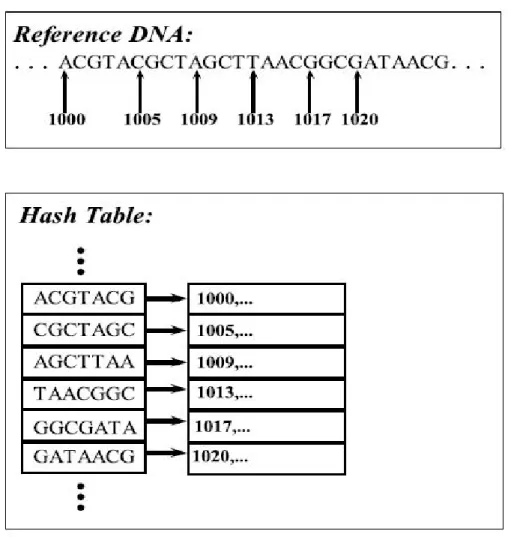
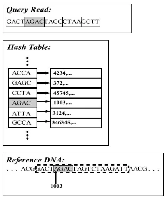
As mentioned above, approaches based on hash based seed and extend are slower than the other paradigm but it tolerates higher error compared to the BWT-FM. This paradigm works in two stages, fast hash table search and alignment [25]. In the first stage, reference fragments are stored in hash table (see Figure 2.6), which their key are chosen among possible seeds that is defined by high similarity re-gion of one read vs one reference segment. The benefit of this method arises from limited search space of selected seed, instead of searching whole genome space. The occurrence of seeds are stored consecutively in another data structure, while they will be used in second stage for extending seed inside selected locations (see Figure 2.7) using dynamic programming techniques. In the following section we

will discuss about Needleman-Wunsch [26], and Smith-Waterman [27] algorithms as an example of dynamic programming approach.

Figure 2.6: Example of hash table for sample data. First, pick k-mer size, and then build lookup for each k-mer as key and their location as value for hash table.

Figure 2.7: Extending the seed from the reference DNA. Compare read hash (seed) to reference hash, then select identical hash hits, and extend read to find best match vs reference fragment in reference genome location.

Optimal alignment algorithms are categorized by local alignment which in-cludes Smith-Waterman algorithm, and global alignments such as Needleman-Wunsch. The calculation of similarity between two pair of sequences are modeled by mathematical equations by considering insertions, deletions, and gap in each process.

2.3.2

Dynamic programming languages

Dynamic programming (DP) techniques solve problems by dividing them into smaller independent sub-problems [28]. These smaller sub-problems are recur-sively divided until solution is trivial, which can be combined to obtain the answer for the entire problem. Optimal solution is determined mostly by one of these objectives: minimization or maximization of a cost function [29, 30]. In dynamic programming techniques, problem is defined as a matrix in which sequences are aligned to a m ∗ n-matrix of subsequences, where row indicate one of the queries with length m, and second one goes for column with length n. The Needleman -Wunsch and Smith-Waterman algorithms are examples of dynamic programming for pairwise alignment, which respectively represent global alignment and local alignment.

2.3.3

Global alignment

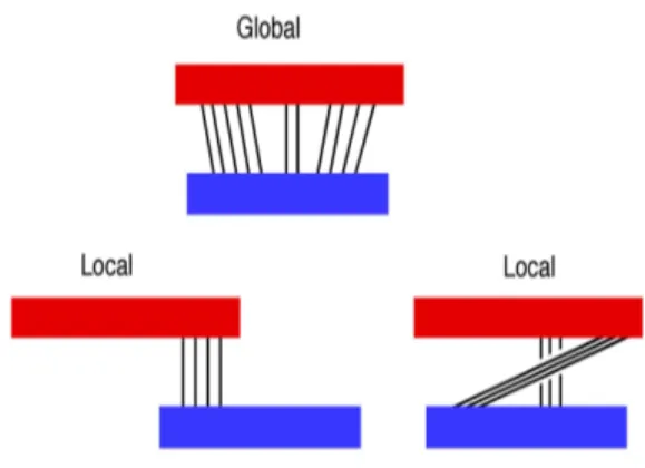
As mentioned earlier, global alignment is used to find optimal alignment that has maximum number of matches, where all characters of both sequences are consid-ered (see Figure 2.8).

Needleman-Wunsch

Needleman-Wunsch algorithm was presented in 1970, in order to search homology of two sequences, where it returns optimal alignment of sequences with maximal number of matches, and is useful when sequences are closely related [26]. Using dynamic programming techniques, similarity score matrix is constructed through which optimal alignment can be identified.

Figure 2.8: An example comparison of global and local alignment.

Initialization

First step of this algorithm begins with initializing matrix for first row and first column filled with a score function which represent gap penalty at start-ing each sequence. Figure 2.9 shows the initialization phase for the sequences ”GAATTCAGTTA” and ”GGATCGA”.

Figure 2.9: Initial alignment matrix of sequences.

Alignment matrix calculation

This step performs calculation in the matrix on F(i,j) depending on F(i-1, j-1) which means match or mismatch, F(i, j-j-1)insertion, or F(i-1, j) deletion. It starts from top left to bottom right corner and it does not matter to proceed in row manner or column manner as long as three dependent cells are available for calculating score of current cell. The highest scoring path is considered for obtaining an optimal alignment. Given the sequence x, and y as queries, the Needleman-Wunsch algorithm performs global alignment through all sequences using equation 2.1. d is the gap penalty.

F (i, j) = max        F (i − 1, j − 1) + s(xi, yj) F (i − 1, j) − d F (i, j − 1) − d (2.1)

with a score function s(ai, bi) defined as equation 2.2.

s(xi, yj) =

(

> 0, xi = yj Match

< 0, xi 6= yj Mismatch

Figure 2.10 shows the example alignment after the matrix fill step. The gap penalty is zero, the score for alignment is 1 and a misalignment is 0. At the end of this phase, score of alignment is retrieved from bottom right cell: in this example, 6.

Algorithm 1 shows the pseudo code for Needleman-Wunsch semi-global align-ment, where the read sequence needs to align with its entire length in order to be mapped successfully.

Algorithm 1 Needleman Wunsch Init and Fill

1: Input: readArray, referenceArray

2: Output: resultMatrix

3: for i = 1 to |readArray| do

4: F(i,0)  0

5: end for

6: for i = 1 to |referenceArray| do

7: F(0,i)  0

8: end for

9: for i = 1 to |readArray| do

10: for j = 1 to |referenceArray| do

11: if referenceArray[i] = readArray[j] then

12: s(𝑥

, 𝑥

)  1

13: else

14: s(𝑥

, 𝑥

)  0

15: end if

16: F(i,j)  max(F(i,j-1)), max(F(i-1,j)), max(F(i-1,j-1))+ s(𝑥

, 𝑥

))

17: end for

Backtracking

Finally, retrieving the global alignment can be determined by a traceback pre-cedure. During matrix fill computing, the choice of movement of each cell is recorded according to above-mentioned formula. In order to find optimal align-ment the traceback can be performed starting at highest value in the last row or last column and iteratively selecting highest value of previous row or column until reach the origin of matrix. If multiple route are possible, there will be multi-ple alignments accordingly. An exammulti-ple of this algorithm is shown in Figure 2.11.

2.3.4

Local alignment

Local alignment is providing the related region of two sequences in pairwise align-ment and can be done with Smith-Waterman-algorithm. Local alignalign-ment is more flexible than global alignment in finding related regions, where they can appear in any order in local alignment whereas this is not possible in global alignment.

Smith-Waterman

Smith-Waterman algorithm was presented in in 1981, in order to find optimal local alignment of pair of sequences, which utilizes dynamic programming algo-rithms. Again this algorithm consist of three steps. First, the first row and column of matrix is filled with zero instead the gap penalties (see Figure 2.13 ). Second, matrix filling is continued by adding zero to the calculation process, in order to find new and better existing alignment (see Figure 2.14). Third, trace-back can be started any places with maximum value and then alignment will be retrieved whenever it reaches to zero (see Figure 2.15).

The scoring function for Smith-Waterman algorithm is shown in Equation 2.3.

F (i, j) = max            0 F (i − 1, j − 1) + s(xi, yj) F (i − 1, j) − d F (i, j − 1) − d (2.3)

Figure 2.12: Initializing similarity score of matrix in Smith-Waterman algorithm.

Figure 2.13: The filled matrix in Smith-Waterman algorithm.

2.4

Graphic Processing Units

Originally, GPUs (Graphics Processing Unit ) [31] were developed as specialized processors for rendering graphics at a time. Graphic task of showing output to display units, is a computationally heavy job, which is applicable in hardware with high requirements. To achieve acceleration, highly parallel processors with limited functionality were introduced, and has been utilized in embedded systems, mobile phones, personal computers, workstations, and game consoles. GPUs have already been shown to be more efficient than CPUs in manipulating massively parallel algorithms, through which many problems in several areas of molecular biology, physics simulation, and scientific computing have been tackled. Figure 2.16 shows a layout of modern GPUs.

Global memory

Shared memory Shared memory

Registers

Device

Multiprocessor Multiprocessor

2.4.1

GPGPU hardware

Streaming multiprocessors

A GPU consists of many Streaming Multiprocessors (SMs) [32], where each of them contains execution units, registers for threads, shared memory, caches, and warp scheduler. Each SM includes many CUDA cores, and instruction cache, warp scheduler and dispatch unit, register file, LD/ST (load/store) units, SFU’s (Special Function Units), and shared memory, through which SM can be effi-ciently used [12] (see Figure 2.16). There are three compute capability 1.x, 2.x, 3.x, which corresponds to Tesla-class, Fermi-class, and Kepler-class respectively, where each of them provide specific features in each generation [33] (see Figure 2.17).

2.4.2

GPGPU programming languages

NVIDIA introduced Compute Unified Device Architecture (CUDA) [33], which is a programming model for general purpose parallel computation that enables scalable and multi-threaded codes to be run on NVIDIA GPUs and has the ex-tension of C language. Nowadays, OpenCL [34], and Microsoft Compute Shader [35] exist that can run on the same hardware; however since CUDA is the most popular and widely used, we will focus on CUDA in this thesis.

CUDA

CUDA performs Single Instruction Multiple Threads (SIMT) model [33], on a single instruction with different data by using parallel threads [33]. A CUDA program starts running on CPU (host code), where it is main program, then CPU retrieves data after execution of kernel (device code) from GPU. The fol-lowing procedure is occurred through most CUDA programming example.

ˆ Host allocates memory for input/output on the device ˆ Host copies input to the device

ˆ Device run the kernel on the set of input data

ˆ Host copies back result from kernel to memory on CPU ˆ Host frees the allocated device memory

Kernels

Aforementioned, a kernel is a program that is run by many parallel processing units of GPU device [33], and declared by adding a prefix “ global ” to a

normal C program [33]. This program, is executed as many time as the size of blocks and threads, which defined in CPU host. Kernel will make use of many variables inside execution time, in order to run parallel threads. These threads are accessible through their built-in variables “threadIdx ”, and it means which threads inside block are running at the time. Also “blockIdx ” variable for each thread is related to the number of block within this thread is running [33]; “block-Dim” provides the information about dimension of block respectively. The simple example of kernel is shown in below.

which can be called in host as shown here:

The compilation process of a GPU-based program, which has both CPU and GPU parts, is shown in figure 2.18.

CUDA Sources C/C++ Sources GCC/G++ GPU Code CPU Code NVCC GCC/G++ C/C++ CUDA

CUDA thread hierarchy

Each CUDA program is executed in a manner shown in Figure 2.19, in which GPU kernel is invoked inside CPU host with symbol <<<>>> within CUDA C/C++ extension code [33]. The kernel is run in parallel fashion N times where N indicates number of specified CUDA threads, where each thread is a processing element of GPU devices. These N threads are invoked by kernel execution and run the same program simultaneously, are called Grid [33]. A kernel is a set of parallel threads that run in SIMD fashion where they execute the same code and each has a private registers and local memory[33]. For a set of 32 threads that execute kernel in parallel, called wrap, it is important to follow the same path to gain full occupancy of GPUs which is demonstrated with no idle thread. At a higher level a set of thread are grouped into block as a multiply of warp size to ensure efficiency of GPU performance [33].

Figure 2.19: Execution of CUDA Kernel [36].

Threads in a grid are categorized in two-level hierarchy [33], which is shown in Figure 2.20. In top-level each grids includes at least one thread block, in which blocks will have the same number of threads, and can be organized in one, two, or three dimensions. These blocks are accessible through kernel execution time

by using their built-in “blockIdx ” variables. The maximum number of thread per block is restricted by the hardware architecture [33]. Also, in multi-GPUs system, on each GPU, kernel can be executed by a grid. The number of block per grid is chosen by programmer and depend to characteristic of GPU devices.

Threads of each block perform kernel in the same multiprocessor in a GPU until completion, where they can utilize shared memory for sharing data among them. Threads of different block can not communicate during the execution of kernel [33].

The total number of threads in whole application are determined by many different factors. One simple idea is to use each thread individually working on a subproblem, but it is also advantageous to use maximum number of threads in at any instance of kernel execution time, in order to not have any idle pro-cessing element. The maximum total number of parallel threads in each GPU device generation is pre-defined and should be considered while programming. A hierarchy of threads in GPU devices is shown in Figure 2.21.

GPU

Grid

Host PC

CUDA memory hierarchy

As mentioned earlier, GPUs consist of multiple streaming multiprocessors (SM) that enable configurable processor array, each containing set of streaming proces-sors (SPs) [33] that consequently comprised of smaller function unit and different levels of memory. In GPU, kernel is designed for running maximum number of concurrent threads which is organized into block and respectively in grid and accesses to data from different memory space in order to increasing occupancy of GPUs.

Memory management is crucial to obtain full efficiency of GPU which in tern can be very complex. GPU memory consist of several different types, size and access time. Size and access time of these different memory types are increas-ing respectively as follows: register memory, shared memory, local memory, and global memory. Global memory of TeslaK20 for our implementation is as much as 6 GB, and local memory which is accessed by only threads and not cached can be the same size as global memory, while all threads access to the same global memory; shared memory is only accessible for threads within the block which also is the fastest memory and has the restriction on its limited size and is a bound for number of concurrent processing queries at the same time on GPUs [33].

Accessing registers and shared memory has been shown to be the fastest, while registers are allocated to individual thread, shared memory is defined for threads within a block. Registers are those private variable of threads which have a life-time of kernel execution. On the other hand, shared memory is designed for sharing data among all threads of block, where they can write and read from it in a fast fashion, and has a lifetime of block execution, and is not accessible by other block. Shared, register, and local memory which can be accessed by threads, are defined inside kernel and reside on-chip in the SM [33].

Global memory is the slowest memory (nearly 100 times slower than shared memory), which has the lifetime of whole application. Also, necessary data can read and write to global memory from CPU host. Since accessing time is much slower than shared memory, its usage should be minimized within the kernel [12]. Global, constant, and texture memory can be allocated in CPU host, similar to global memory, constant and texture memory are declared in global scope and have the application lifetime, and cannot be written within kernel execution time. Constant and texture memory are cached and obviously faster than global memory, but they are limited in size compare to global memory. Figure 2.22 shows the memory hierarchy for threads in GPUs.

Figure 2.22: Memory Hierarchy for threads [32].

Thread synchronization

In order to avoid simultaneous read/write by threads within a block in shared memory, CUDA provides a mechanism called syncthreads(), by which threads should wait for other to terminate their task, where their results are needed by other threads in the next step of kernel execution time.

Chapter 3

Related Work

Most of the available algorithms for read mapping are CPU-based, and they require very long running times (30-100 CPU days per genome). There is an extensive survey [37] discussing mainly about alignment algorithms and CPU-based mappers as well.

There are few works on read mapping algorithms that utilize GPUs for par-allelism. Manavaski et al. [38] have accelerated different approaches for DNA alignments using Smith-Waterman algorithm on GPUs, but their method is lim-ited in performance gains. Schatz et al. [39] have implemented a local sequence alignment algorithm (MUMmer) on GPU which is a CUDA accelerated version of the MUMmer approach [40] with 10 fold speed-up over the CPU version. Similarly, a parallel implementation of Smith- Waterman algorithm is provided in CUDASW++ [41]; however it has limitations on maximum read length and refer-ence sequrefer-ence due to GPU memory usage. Bowtie [42] is a fast short read-aligner which is based on approximate matching using Burrows-Wheeler Transform [21], but it is limited on error threshold, which makes it not appropriate for sequences with many gaps or high error. CUDAlign [42] is a GPU implementation for pair-wise sequence alignment of only two large sequences with more than a million bases.

Some GPGPU-based aligners, such as CUSHAW [43], a CUDA-enabled GPU implementation with no support of gapped alignments, utilizes BWT-FM [21, 44], which is not suitable for GPGPUs, since the core of the BWT-FM alignments is binary search that causes many divergent branch operations. Even if BWT-FM is used only on the CPU-side to find seed locations quickly instead of hash tables, this often results in a non-uniform sequence length for the verification step, which in turn causes non-uniform thread utilization and significant branch divergence. Thus, it will be better use hash tables to identify short seeds, fol-lowed with millions of concurrent alignments of the same size in GPGPUs that enable full thread synchronization. SOAP3/GPU [45] is also a CUDA-enabled GPU implementation of SOAP [46], but similar to CUSHAW, it does not allow gapped alignments. Furthermore, a thorough discussion on GPU-based aligners is provided in a survey [47].

Chapter 4

Implementation

In this chapter, we will introduce our massively parallel semi-global alignment implementation for DNA sequences which provide significant speed-up over CPU implementation. In order to satisfy the requirements of hash based seed and ex-tend method, we propose a Needleman-Wunsch-based GPU optimized algorithm, that can compute thousands of dynamic programming matrices simultaneously. This implementation can be integrated to other programs in their alignment phase. CPU host, specifies reads and reference segment locations, and sends them to GPU, and computed results are sent back to CPU as a 1D array. In order to eliminate redundant calculations, Ukkonen’s algorithm [48] is performed and no dependencies ensure maximum speed-up and concurrency in GPU pro-gram.

To design our GPU-based short read alignment we utilizes namely Compute Unified Device Architecture CUDA [33] that is a parallel architecture with prop-erty of setting threads structure and memory hierarchy, which in tern used to parallelizes our read alignment part in C code. CUDA platform is programmed with extension of C programming language and CUDA programming is comprised of two separate parts called host and device. Kernel is a light program that is

blocks and respectively a grid of blocks executed in device and called from host. It is crucial to determine scalable configuration for threads hierarchy and mem-ory hierarchy in order to obtain efficient performance of GPUs, which depends on considering different levels of memory, programming model, and parallel algo-rithm.

First, at the start of execution time, the portion of current reference and read sequences are loaded into GPU global memory. This data will be used by GPU alignment kernel, where the aligning of million reads and reference fragments di-vided into thousands of blocks and hundreds of processors. Result of kernel once finishes, will transferred from GPU to CPU for further processing. The order of tasks which performed in GPU is given below:

ˆ GPU initialization ˆ Memory allocation

ˆ Host to Device data copy ˆ Kernel launch

ˆ Memory de-allocation

ˆ Time-measurement in GPU

Following section will describe more details of each step that is performed in our implementation.

4.1

Parallelism and data dependencies

As mentioned above, SIMD structure has been used in GPU-based algorithms which enables program to divide the workload among many threads. The strategy is used here, assigns maximum number of independent threads to each alignment matrix with minimum usage of shared memory in GPU, which ensures maximum occupancy on GPU. The threads that are responsible for calculating of one align-ment matrix, share their result through shared memory whenever it is necessary. The number of assigned threads are determined by error threshold set by user, which is equal to 2e+1. Additionally, these threads are performing loading and copying data from global memory to shared memory at the beginning of the pro-gram. For calculating in each cell Fi,j, as discussed in section 2, considering three

cells Fi−1,j−1, Fi−1,j, Fi,j−1is required, which brings two major strategies for order

of cell computation as shown in Figure 4.1, and 4.2.

Figure 4.2: Column by column strategy.

In these two methods [49], each cell Fi,j is dependent to previous cell, therefore,

only one thread can traverse through cells in order to minimize latency. To obtain parallel computation through each alignment matrix, anti diagonal order can be utilized, which is shown in Figure 4.3. This approach, unlike the others, performs computation from top-left and continues until bottom-right, in such a way that, number of computing cells in each iteration is increased and they are independent to each other, which enables N parallelism for N cells in each iteration. Although, this method shows a N parallelism, but different number of cells per iteration is not suitable for occupancy on GPU, since CUDA considers maximum number of cells per anti-diagonal, and threads are idle in those iteration with less number of cells.

4.2

Ukkonen’s edit distance

In regular matrix alignment calculation, all cells need to be computed in order to find optimal alignment; although, for certain conditions computing all cells is redundant and should be eliminated to gain faster results. Considering Leven-shtein’s edit distance algorithm [14], computing some cells are not required to obtain optimal alignment, which reflects in DNA sequence alignment with lim-ited error threshold, where many cells in matrices can be omitted. Based on Ukkonen’s algorithm, also considering Levenshtein edit distance [14], backtrack-ing path matches to one of diagonal in alignment matrix, where it can cover e (maximum error threshold) neighbourhood of main diagonals. This explanation is demonstrated in Figure 4.4, where error threshold is equal to three.

Figure 4.4: Ukkonen’s edit distance algorithm. Shaded cell are calculated along-side main diagonal.

The benefit of using Ukkonnen’s edit distance, comes from less computed cells per matrix alignment, and also equal number of cell per anti-diagonal in most of iterations, which these advantages ensure better performance on GPUs.

4.3

Anti-diagonal parallelism

Aligning large dataset of reads against huge reference genome, requires hundreds of CPU days to be performed, therefore, our main goal is to design a parallel alignment precedure to reduce the computation time.

In our method, we perform millions of alignment in one execution of kernel in GPU, which its algorithm lies on anti-diagonal parallelism. Each query is assigned to one matrix, and reference segments plus 2e are aligned with short reads by using 2e + 1 threads, where it indicates width of anti-diagonal alongside its neighbourhoods.

In order to avoid branch divergence that leads to low speed execution and also lower efficiency, diagonal approach can go through independent routes that satisfies maximum parallelization for threads while all assigned threads follow the same execution path which ensures minimum branch divergence.

Figure 4.5: Memory Hierarchy for threads.

Finding minimum edit distance for each query is dependent of previous anti-diagonal result as shown in Figure 4.5. Due to large size of data and limited size

of shared memory, these data need to be stored in global memory, where slow ac-cess time to global memory decrease performance of GPU drastically; meanwhile it introduces subsequent memory bandwidth occupancy challenge. To overcome this problem, we used shared memory as a temporary space to hold results as long as they are relevant to the next step (anti-diagonal), which minimizes re-quested shared memory dramatically and allows devices to maximize number of concurrent queries per GPU devices that is scaled by many factors include shared memory usage.

The proposed method exploits CUDA thread hierarchy, in which threads are organized in matrices to calculate each matrix alignment in anti-diagonal fash-ion. Respectively, many matrices are organized in blocks, and are processed in parallel with other matrices in the same block. Considering any error threshold, number of threads automatically is changed per matrix, and consequently num-ber of matrices per block, to ensure maximum occupancy on GPU device. These characteristics are determined in beginning of program based on GPU device gen-eration and available memory.

4.4

CUDA optimization

Alignment process is mapping a read to a reference fragment which is processed independently from any other set of sequences, since it does not require any other information from other mapping, GPU can employ data parallelism with consid-ering hundreds of thousands threads simultaneously for kernel that assign 2e + 1 threads where e denotes error threshold, to each individual mapping process, therefore number of threads for each kernel run, should be a multiple of all these three variables: blocks, threads within block and (2e + 1).

4.4.1

Kernel run for alignment task

The alignment kernel for our implementation in the first step employs hundreds of thousands of threads in parallel in order to identify the minimum error thresh-old for mapping sequences, where it is shown to be most-time consuming part of total execution time in CPU aligner based on profiling conducted in FastHASH [25], which most mapping sequences fail to pass this error threshold(verification step). Parallelization are performed to achieve speedup in verification step by using kernel function in a set of million threads which access data in different memory spaces and follow the same path for identifying minimum edit distance.

Data is maintained in global memory of GPU devices once kernel execution starts, and then transferred to shared memory, at the same time by using all number of threads per block. Storing data in adjacent shared memory locations, guarantees no idle thread in GPU devices which leads to higher throughput. Each thread uses its own unique identifier namely called “threadIdx.x ” that is utilized by our implementation which means: accessing (write/read respectively) consecutive memory location in global memory and shared memory, will be per-formed by consecutive threads that is considered as the important strategy for increasing performance of GPUs [12]. Each fragment of read and reference is transferred as one dimensional array by dividing fixed given size of fragment to the number of specified threads for each queries which is equal to 2e + 1 where e is achieved from user request at beginning of program. In our implementation number of total threads is bounded by number of queries multiplied by 2e + 1. Shared memory is the constraint for number of concurrent queries per block as it has a limited size and show fast access, therefore storing read and reference fragments in shared memory imposes some limitations that should be considered in programming model. Thus the maximum number of queries is achievable in our program by considering available memory of device generation which subse-quently determines other dependent variables of our program.

Search traversal will perform by 2e+1 threads for each read and reference map-ping query bounded by Ukkonene’s approximation algorithm [48] edit distance which allows us to reduce search space and indicates that we only require to tra-verse in each row and column as many as error threshold. Utilizing thousands of concurrent threads assigns very limited memory to each thread, therefore the computations rather than storing all steps and results in shared memory, should be performed in such a way that requires minimum storing amount of results. Therefore we developed a method that satisfies constraints by Ukkonen’s ap-proximation and obtains the maximal parallelization among threads (row major, column major, diagonal major).

4.4.2

Transferring whole reads and reference sequences

into global memory

In order to minimize time spent in initialization step for kernel function, first in mrFAST [50] CPU-side, total reads and a chunk of reference sequences related to each chromosome are represented in a one dimensional array (this ensures fast data access by threads). Then this data will be transferred once to global mem-ory of GPU, while residing in device will subsidize transferring time, it can also serve one million related queries until finishing aligning all reads and references fragment in verification step.

4.4.3

Transferring pointers of reads and reference

frag-ments for current kernel

One dimensional array of pointers to the locations of read and reference queries in global memory will be sent to each kernel of GPU devices, and obtains drastic reduction in transferring time and higher throughput in our application.

4.4.4

Multi-GPU design

Our GPU aligner identifies all number of GPU devices once CPU program starts, each of which operates proportionally on part of processing data, which in turn propagates the workload concurrently between available devices. As mentioned earlier, data for GPU devices transferred once and reside in global memory and then many batches of queries will be processed until data discarded from CPU thread for next transferring read and reference buffers, which obtains minimum transferring time and increases efficiency of GPU devices.

4.4.5

Transferring result from GPU to disk

Read and reference sequences that are divided to available GPU devices will per-form kernel execution and after processing, their minimum edit distance result will be collected and transferred to CPU and combined with other results from other devices. During execution of each kernel, sequences of read and reference and their calculated edit distance will temporarily store in shared memory of GPU, since shared memory is accessible at the run-time of each block, once the execution of each block finishes, result will be copy to global memory and sub-sequently copy from global memory of GPU back to CPU after execution of kernel.

Chapter 5

Results

In this chapter, we evaluate the performance of the GPU-based Needleman-Wunsch. Section 5.1 details the benchmarking environment, and section 5.2 presents experimental results and provides comparison with CPU-based aligner.

5.1

Benchmarking environment

We implemented our methods using CUDA version 7.5 on NVIDIA Tesla K20, then we integrated our approach with a popular hash-table based read mapping algorithm, mrFAST [50]. Our methods help substantially ameliorate the compu-tational burden of HTS data analysis, a much needed improvement over current methods.

Development system 2 x 8 Cores, Intel(R) Xeon(R) CPU E5-2643 0 (3.30GHz) CPU with level-2 cache of size 10 Mbytes and 3 TB local disk, and NVIDIA Tesla K20 GPU with 6 GB of memory. There are 336 shader (CUDA) cores for parallel computation each is 1620-1900 MHz. This graphics card had clock speed of 633, 1134 and 1404 MHz for its core, memory and shaders respec-tively. The CUDA toolkit used was version 7.5.

Database In our experiment, we used human genome as reference for compu-tation which we divided it chunk by chunk and stored in GPU memory as one dimensional array. Each chunk of human reference remain until all related data are processed in GPU, then we replace next chunk so on. In each execution, we determine millions of location in the genome and send them to GPU for fetch-ing data from those locations to GPU shared memory for processfetch-ing, where each single processing needs a size of N + 2e from specified location.

Query sequences We store the WGS reads at once as one dimensional array in GPU global memory and they reside there until the program ends. Each read is represented as size of N and processed against references with size of N+2e. Locations of these reads are determined by CPU host (mrFAST).

The run-time of program is calculated by C clock() instruction; and accuracy of results are verified by mrFAST output results. Storing data and copying results into/from GPU is not included in the measuring time. Result evaluated in both CPU-implementation mrFAST and GPU-friendly for a number of different reads queries measured in paired-end mode.

5.2

Performance results

In this part, we discuss and compare results of performance of GPU implementa-tion of parallel algorithm described in secimplementa-tion 4 and CPU implementaimplementa-tion without considering data transfer time to/from GPU memory. It should be mentioned that, for available-GPU design speed-up is multiplied by number of GPU devices running on the system.

The first experiment, shows the performance of three different settings for GPU-based algorithm where 32, 64 and 100 matrices per block are considered

against CPU-based implementation, where we consider early termination strat-egy in GPU execution for threads to reduce the overall runtime of program, which means in each anti-diagonal execution, threads check if they have passed error threshold to exit early or not. Number of matrices M indicated number of align-ments each contains one read and one reference. The error threshold is 4 in each alignment for both CPU and GPU implementation, and number of threads are defined as 2e + 1 for each matrix in GPU algorithm. The maximum number of allowed matrices per block is 100 for the device we used in our experiment which we obtain by considering read length and error threshold.

The maximum number of block in each experiment identified by device char-acterization; however this number is not a critical variable in our design. Total number of thread is equal to M ∗ (2e + 1), where M indicates total number of alignment matrices and e stands for error threshold.

Number of Matrices 20K 200K 240K 440K 2M 4M 8M 16M 24M 30M 40M Running time (ms.) 0 2000 4000 6000 8000 10000 12000 14000 16000 18000 CPU

GPU with 100 matrices/block GPU with 64 matrices/block GPU with 32 matrices/block

Figure 5.1: The comparison between CPU and three setting for GPU. (Read Size:50, Reference Segment Size: 58, Error Threshold:4)

Figure 5.1, shows that the runtime of CPU-based algorithm increases substan-tially compare to GPU-based performance. All GPU-based experiments show almost same performance against CPU-based algorithm and clearly point out they are more efficient than CPU-based implementation.

The corresponding speed-up related to three setting for GPU-based approach is measured in percentage compare to CPU implementation. Table 5.1 shows the testing results of our experiment.

Number of Alignment Matrices Running Time (ms.) Speed-up 1 GPU Speed-up 2 GPU CPU 32 M/B GPU 64 M/B GPU 100 M/B GPU 20,000 10.93 0.39 0.49 0.50 95.77% 23.95 47.91 200,000 94.57 3.34 3.97 4.44 95.85% 24.47 48.95 240,000 112.55 4.08 4.75 5.31 95.81% 24.14 48.29 440,000 202.24 7.46 8.61 9.63 95.76% 23.86 47.72 2,000,000 836.39 30.20 35.36 40.01 95.79% 24.08 48.16 4,000,000 1785.33 66.95 75.54 89.67 95.66% 23.40 46.81 8,000,000 3250.59 120.46 139.48 160.85 95.68% 23.49 47.00 16,000,000 7096.49 262.28 306.29 350.63 95.68% 23.48 46.98 24,000,000 10712.20 396.31 467.62 531.47 95.65% 23.36 46.73 30,000,000 13984.16 518.28 606.45 699.81 95.65% 23.34 46.68 40,000,000 16855.93 628.52 741.22 847.10 95.61% 23.15 46.30

Table 5.1: The comparison between CPU version aligner and three setting for GPU-based method. (Read Size:50, Reference Segment Size: 58, Error Thresh-old:4)

Figure 5.2 shows the effect of different number of matrices per blocks where 32 matrices per block performance is better than 64 and 100 matrices per block. The reason for this can be explained by synchronization of fewer threads at each block, where synchronization forces all threads of block to stop because of unfinished threads; therefor less threads per block means higher probability for starting new execution for threads in the previous stage.

Number of Matrices 20K 200K 240K 440K 2M 4M 8M 16M 24M 30M 40M Speed up 18 20 22 24 26 28 30 100 matrix/block 64 matrix/block 32 matrix/block

Figure 5.2: The comparison between three different setting for GPU approach in various number of threads per block. (Read Size:50, Reference Segment Size: 58, Error Threshold:4)

For the following results, we did not consider early termination strategy in our experiments. We consider GPU experiments with 32, 64, 100 number of matri-ces per block and error threshold set to 4. Total number of thread is equal to M ∗ (2e + 1), where M indicates total number of alignment matrices and e stands for error threshold. Figure 5.3, shows the runtime of CPU-based aligner against three different setting for GPU-based approach.

Number of Matrices 20K 200K 240K 440K 2M 4M 8M 16M 24M 30M 40M Running time (ms.) 0 2000 4000 6000 8000 10000 12000 14000 16000 18000 CPU

GPU with 100 matrices/block GPU with 64 matrices/block GPU with 32 matrices/block

Figure 5.3: The comparison between CPU version aligner and three different setting for GPU-based approach. (Read Size:50, Reference Segment Size: 58, Error Threshold:4)

The average speed-up gained in three GPU-based experiments over CPU ver-sion is shown in Table 5.2, which shows drastic reduction compare to previous measurement and it is obviously occur because threads should continue to the end of matric regardless of computed error threshold.

Number of Alignment Matrices Running Time (ms.) Speed-up 1 GPU Speed-up 2 GPU CPU 32 M/B GPU 64 M/B GPU 100 M/B GPU 20,000 10.93 1.44 1.60 1.68 85.58% 6.96 13.93 200,000 94.57 13.22 14.34 15.12 84.94% 6.66 13.33 240,000 112.55 15.03 17.21 18.05 85.10% 6.75 13.51 440,000 202.24 28.02 30.18 32.96 84.97% 6.68 13.37 2,000,000 836.39 112.58 127.99 136.95 84.95% 6.69 13.38 4,000,000 1785.33 264.33 271.47 307.13 84.26% 6.38 12.76 8,000,000 3250.59 448.07 512.14 550.91 84.50% 6.50 13.00 16,000,000 7096.49 966.11 1101.55 1202.38 84.64% 6.56 13.13 24,000,000 10712.20 1479.78 1688.21 1829.23 84.45% 6.48 12.96 30,000,000 13984.16 1945.33 2221.05 2423.90 84.29% 6.41 12.84 40,000,000 16855.93 2359.16 2690.82 2922.85 84.23% 6.39 12.78

Table 5.2: GPU implementation speed-up over CPU version. (Read Size:50, Reference Segment Size: 58, Error Threshold:4)

Figure 5.4, shows the impact of different number of matrices per block in second experiment. Number of Matrices 20K 200K 240K 440K 2M 4M 8M 16M 24M 32M 40M Speed up 5.5 6 6.5 7 7.5 8 100 matrix/block 64 matrix/block 32 matrix/block

Figure 5.4: The comparison between three different GPU setting in various num-ber of threads per block. (Read Size:50, Reference Segment Size: 58, Error Threshold:4)

Chapter 6

Conclusion

Basically, our approach is to move the compute-intense but embarrassingly par-allel verification step to the GPGPUs. We perform the hash table lookup for seed location in the CPU in O(1) time per seed [50]. We collect the seeds in a buffer, which we then passed to the GPGPU for millions of simultaneous alignments. The number of alignments are automatically determined by considering the char-acteristics of the GPGPU such as available shared memory, which has an effect on the number of threads, blocks, grid and other variables in GPUs. The number of threads used per alignment is adjusted dynamically based on the maximum allowed error threshold set by the user.

There are several characteristics of our approach that makes our new mapping mechanism beneficial in multiple ways. First, we mapped a time-consuming appli-cation to massively parallel GPU architectures, providing a significant speed-up that will dramatically decrease the time required for DNA sequence analysis. Sec-ond, our approach easily can be merged with any existing and future hash-table based read mapping applications. Third, our algorithms can be used for various configurations like different read sizes, reference genome size and error allowance. This provides a high flexibility of processing the outputs of different sequencing

we reduced host to GPU transfer time significantly by placing all relevant data to the GPU global memory in the initialization step. This helps us eliminate the need to re-transfer the same reads for different seed locations, and reference genome segments for different reads.

Here, we developed and implemented a GPGPU-friendly algorithm based on Levenshtein’s algorithm [14] that can compute millions of dynamic programming matrices concurrently. We implemented our algorithms using the CUDA (Com-pute Unified Device Architecture) platform, and test them using the NVIDIA Tesla K20 GPGPU processors. In this work, we propose a massively parallel, fast, memory-aware Levenshtein edit distance algorithm model for graphics pro-cessing units, together with Ukkonen’s approximation algorithm [48] to prevent redundant calculations in matrices. Considering the memory limitations and very high number of available threads, our algorithm ensures maximum occupancy on GPGPUs. Our experimental results show significant speedup over CPU-based aligners.

Bibliography

[1] N. J. Loman, C. Constantinidou, J. Z. Chan, M. Halachev, M. Sergeant, C. W. Penn, E. R. Robinson, and M. J. Pallen, “High-throughput bacterial genome sequencing: an embarrassment of choice, a world of opportunity,” Nature Reviews Microbiology, vol. 10, no. 9, pp. 599–606, 2012.

[2] F. Antonacci, J. M. Kidd, T. Marques-Bonet, M. Ventura, P. Siswara, Z. Jiang, and E. E. Eichler, “Characterization of six human disease-associated inversion polymorphisms,” Human molecular genetics, vol. 18, no. 14, pp. 2555–2566, 2009.

[3] J. A. Bailey, A. M. Yavor, H. F. Massa, B. J. Trask, and E. E. Eichler, “Segmental duplications: organization and impact within the current human genome project assembly,” Genome research, vol. 11, no. 6, pp. 1005–1017, 2001.

[4] F. Antonacci, J. M. Kidd, T. Marques-Bonet, B. Teague, M. Ventura, S. Giri-rajan, C. Alkan, C. D. Campbell, L. Vives, M. Malig, et al., “A large and complex structural polymorphism at 16p12. 1 underlies microdeletion disease risk,” Nature genetics, vol. 42, no. 9, pp. 745–750, 2010.

[5] J. A. Bailey and E. E. Eichler, “Primate segmental duplications: crucibles of evolution, diversity and disease,” Nature Reviews Genetics, vol. 7, no. 7, pp. 552–564, 2006.

[6] J. A. Bailey, Z. Gu, R. A. Clark, K. Reinert, R. V. Samonte, S. Schwartz, M. D. Adams, E. W. Myers, P. W. Li, and E. E. Eichler, “Recent segmental

duplications in the human genome,” Science, vol. 297, no. 5583, pp. 1003– 1007, 2002.

[7] J. Bailey, J. Kidd, and E. Eichler, “Human copy number polymorphic genes,” Cytogenetic and genome research, vol. 123, no. 1-4, pp. 234–243, 2009. [8] E. S. Lander, L. M. Linton, B. Birren, C. Nusbaum, M. C. Zody, J. Baldwin,

K. Devon, K. Dewar, M. Doyle, W. FitzHugh, et al., “Initial sequencing and analysis of the human genome,” Nature, vol. 409, no. 6822, pp. 860–921, 2001.

[9] J. C. Venter, M. D. Adams, E. W. Myers, P. W. Li, R. J. Mural, G. G. Sutton, H. O. Smith, M. Yandell, C. A. Evans, R. A. Holt, et al., “The sequence of the human genome,” science, vol. 291, no. 5507, pp. 1304–1351, 2001.

[10] M. Pop and S. L. Salzberg, “Bioinformatics challenges of new sequencing technology,” Trends in Genetics, vol. 24, no. 3, pp. 142–149, 2008.

[11] F. De Bona, S. Ossowski, K. Schneeberger, and G. R¨atsch, “Optimal spliced alignments of short sequence reads,” BMC Bioinformatics, vol. 9, no. Suppl 10, p. O7, 2008.

[12] NVIDIA., “Cuda c best practices guide. website, dg-05603-001 v5.5.,” 2014. [13] C. Alkan, J. M. Kidd, T. Marques-Bonet, G. Aksay, F. Antonacci, F. Hor-mozdiari, J. O. Kitzman, C. Baker, M. Malig, O. Mutlu, et al., “Person-alized copy number and segmental duplication maps using next-generation sequencing,” Nature genetics, vol. 41, no. 10, pp. 1061–1067, 2009.

[14] V. I. Levenshtein, “Binary codes capable of correcting deletions, insertions and reversals,” in Soviet physics doklady, vol. 10, p. 707, 1966.

[15] M. Plus, “Medical encyclopedia: Dna-structure retrieved online on aug. 9, 2007 from the internet: https://ghr.nlm.nih.gov/primer/basics/dna. html,” [16] G. J. Tortora and B. H. Derrickson, Principles of anatomy and physiology.

[17] K. Pr¨ufer, K. Munch, I. Hellmann, K. Akagi, J. R. Miller, B. Walenz, S. Ko-ren, G. Sutton, C. Kodira, R. Winer, et al., “The bonobo genome com-pared with the chimpanzee and human genomes,” Nature, vol. 486, no. 7404, pp. 527–531, 2012.

[18] S. Brenner, M. Johnson, J. Bridgham, G. Golda, D. H. Lloyd, D. Johnson, S. Luo, S. McCurdy, M. Foy, M. Ewan, et al., “Gene expression analysis by massively parallel signature sequencing (mpss) on microbead arrays,” Nature biotechnology, vol. 18, no. 6, pp. 630–634, 2000.

[19] K. Runte, “A brief introduction to genomics research retrieved online on jul. 30, 2016 from the internet: https://wiki.cebitec.uni-bielefeld.de/brf-software/index.php/gendbwiki/introductiontogenomics. html,” tech. rep. [20] R. Edgar, “Fastq files retrieved online on jul. 30, 2016 from the internet:

http://drive5.com/usearch/manual. html,” tech. rep.

[21] M. Burrows and D. J. Wheeler, “A block-sorting lossless data compression algorithm,” 1994.

[22] J. Pevsner, Bioinformatics and functional genomics. John Wiley & Sons, 2015.

[23] P. Ferragina, G. Manzini, V. M¨akinen, and G. Navarro, “Compressed repre-sentations of sequences and full-text indexes,” ACM Transactions on Algo-rithms (TALG), vol. 3, no. 2, p. 20, 2007.

[24] S. F. Altschul, W. Gish, W. Miller, E. W. Myers, and D. J. Lipman, “Basic local alignment search tool,” Journal of molecular biology, vol. 215, no. 3, pp. 403–410, 1990.

[25] H. Xin, D. Lee, F. Hormozdiari, S. Yedkar, O. Mutlu, and C. Alkan, “Accel-erating read mapping with fasthash,” BMC genomics, vol. 14, no. Suppl 1, p. S13, 2013.

[26] S. B. Needleman and C. D. Wunsch, “A general method applicable to the search for similarities in the amino acid sequence of two proteins,” Journal

[27] T. F. Smith and M. S. Waterman, “Identification of common molecular sub-sequences,” Journal of molecular biology, vol. 147, no. 1, pp. 195–197, 1981. [28] P. Baldi and S. Brunak, Bioinformatics: the machine learning approach.

MIT press, 2001.

[29] E. W. Myers and W. Miller, “Optimal alignments in linear space,” Computer applications in the biosciences: CABIOS, vol. 4, no. 1, pp. 11–17, 1988. [30] P. Viola and W. M. Wells III, “Alignment by maximization of mutual

infor-mation,” International journal of computer vision, vol. 24, no. 2, pp. 137– 154, 1997.

[31] M. Garland, S. Le Grand, J. Nickolls, J. Anderson, J. Hardwick, S. Morton, E. Phillips, Y. Zhang, and V. Volkov, “Parallel computing experiences with cuda,” Micro, IEEE, vol. 28, no. 4, pp. 13–27, 2008.

[32] N. Wilt, “The cuda handbook : A comprehensive guide to gpu program-ming.,” June 2013.

[33] NVIDIA Corporation, CUDA C Programming Guide Version 4.0, 2011. NVIDIA Corporation, 2011.

[34] J. E. Stone, D. Gohara, and G. Shi, “Opencl: A parallel programming stan-dard for heterogeneous computing systems,” Computing in science & engi-neering, vol. 12, no. 1-3, pp. 66–73, 2010.

[35] Microsoft., “Compute shader overview.,” 2013.

[36] D. B. Kirk and W. H. Wen-mei, Programming massively parallel processors: a hands-on approach. Newnes, 2012.

[37] H. Li and N. Homer, “A survey of sequence alignment algorithms for next-generation sequencing,” Briefings in bioinformatics, vol. 11, no. 5, pp. 473– 483, 2010.

[38] S. A. Manavski and G. Valle, “Cuda compatible gpu cards as efficient hard-ware accelerators for smith-waterman sequence alignment,” BMC bioinfor-matics, vol. 9, no. 2, p. 1, 2008.