Detection of tree trunks as visual landmarks in outdoor environments

ENVIRONMENTS

a thesis

submitted to the department of computer engineering

and the institute of engineering and science

of bilkent university

in partial fulfillment of the requirements

for the degree of

master of science

By

Tu˘gba Yıldız

August, 2010

Assist. Prof. Dr. Uluc. Saranlı(Advisor)

I certify that I have read this thesis and that in my opinion it is fully adequate, in scope and in quality, as a thesis for the degree of Master of Science.

Assist. Prof. Dr. Selim Aksoy

I certify that I have read this thesis and that in my opinion it is fully adequate, in scope and in quality, as a thesis for the degree of Master of Science.

Assist. Prof. Dr. Afs.ar Saranlı

Approved for the Institute of Engineering and Science:

Prof. Dr. Levent Onural Director of the Institute

LANDMARKS IN OUTDOOR ENVIRONMENTS

Tu˘gba Yıldız

M.S. in Computer Engineering Supervisor: Assist. Prof. Dr. Uluc. Saranlı

August, 2010

One of the basic problems to be addressed for a robot navigating in an outdoor environment is the tracking of its position and state. A fundamental first step in using algorithms for solving this problem, such as various visual Simultaneous Localization and Mapping (SLAM) strategies, is the extraction and identifica-tion of suitable staidentifica-tionary “landmarks” in the environment. This is particularly challenging in the outdoors geometrically consistent features such as lines are not frequent. In this thesis, we focus on using trees as persistent visual landmark features in outdoor settings. Existing work to this end only uses intensity infor-mation in images and does not work well in low-contrast settings. In contrast, we propose a novel method to incorporate both color and intensity information as well as regional attributes in an image towards robust of detection of tree trunks. We describe both extensions to the well-known edge-flow method as well as com-plementary Gabor-based edge detection methods to extract dominant edges in the vertical direction. The final stages of our algorithm then group these vertical edges into potential tree trunks using the integration of perceptual organization and all available image features.

We characterize the detection performance of our algorithm for two different datasets, one homogeneous dataset with different images of the same tree types and a heterogeneous dataset with images taken from a much more diverse set of trees under more dramatic variations in illumination, viewpoint and background conditions. Our experiments show that our algorithm correctly finds up to 90% of trees with a false-positive rate lower than 15% in both datasets. These results establish that the integration of all available color, intensity and structure infor-mation results in a high performance tree trunk detection system that is suitable for use within a SLAM framework that outperforms other methods that only use image intensity information.

Keywords: Edge detection, perceptual grouping, color, Gabor wavelets, object

detection, tree trunk detection, visual landmarks, visual SLAM, computer vision, pattern recognition, image processing.

. ORTAMLARDA G

. ARETLER

OLARAK A ˘

GAC

_{. G}

OVDELER˙IN˙IN TESP˙IT˙I

¨

Tu˘gba Yıldız

Bilgisayar M¨uhendisli˘gi, Y¨uksek Lisans Tez Y¨oneticisi: Assist. Prof. Dr. Uluc. Saranlı

A˘gustos, 2010

Dıs. ortamda, robotun konumunun ve durumunun takip edilmesi, robotun nav-igasyonu ic.in ele alınması gereken temel sorunlardan biridir. Bu problemi c.¨ozebilmek ic.in kullanılan, c.es.itli G¨or¨unt¨u Tabanlı Es. Zamanlı Lokalizasyon ve Harita C.ıkarma (visual SLAM) stratejileri gibi algorithmaların ilk temel adımı ortamda bulunan uygun sabit “yer is.aretc.ilerinin” saptanması ve c.ıkarılmasıdır. Fakat dıs. ortamda bulunması gereken geometrik olarak tutarlı c.izgiler gibi ¨ozelliklerin sık bulunmaması, robotun navigasyonunu zorlas.tırmaktadır. Bu tez c.alıs.masında, dıs. ortamlarda s¨urekli g¨orsel yer is.areti ¨ozellikleri olarak a˘gac.ların kullanılmasına odaklanılmaktadır. _{Bu amac.la yapılan c.alıs.malarda sadece} g¨or¨unt¨ulerdeki yo˘gunluk bilgisi kullanılmakta ve d¨_{us.¨uk kontrast ayarlarında bu} c.alıs.maların yeterli seviyede sonuc. vermedi˘gi g¨ozlemlenmis.tir. Buna kars.ılık, c.alıs.mamızda a˘gac. g¨ovdelerinin stabil algılanmasına y¨onelik g¨or¨unt¨ude, renk ve yo˘gunluk bilgilerini, b¨olgesel ¨ozellikleri ile birles.tiren yeni bir y¨ontem ¨oneriyoruz. Dikey y¨onde bulunan baskın kenarları c.ıkarmak ic.in iyi bilinen kenar-akıs.ı (edge-flow) y¨onteminin yanı sıra, tamamlayıcı Gabor tabanlı kenar belirleme y¨ontemine uyguladı˘gımız de˘gis.iklikleri ac.ıkladık. Algoritmamızın son as.amalarında algısal organizasyon ve mevcut t¨um g¨or¨unt¨u ¨ozelliklerinin entegrasyonu kullanılarak bu dikey kenarlar potansiyel a˘gac. g¨ovdeleri olarak gruplanır.

Algoritmamızın algılama performansını karakterize edebilmek ic.in biri homo-jen di˘geri heterohomo-jen olmak ¨uzere iki farklı veri k¨umesi kullandık. Bunlardan ilki, aynı a˘gac. t¨urlerinden alınan farklı g¨or¨unt¨ulerden olus.mus.tur. Di˘gerinde ise aydınlatma, bakıs. ac.ısı ve arka plan kos.ullarında daha dramatik de˘gis.imler altında a˘gac.ların farklı t¨urlerinden alınan g¨or¨unt¨uler yer almaktadır. Deneylerimiz, algo-ritmamızın her iki veri k¨umesinde de 15% den daha d¨_{us.¨uk yalancı pozitiflik oranı} ile a˘gac.ların 90% kadarını do˘gru olarak buldu˘gunu g¨ostermektedır. Deneyimiz,

sadece g¨or¨unt¨u yo˘gunlu˘gu bilgileri kullanan di˘ger y¨ontemlerden ¨ust¨un olan, mev-cut renk, yo˘gunluk ve yapı bilgisinin entegrasyonu ile tasarlanmıs. ve bir SLAM c.erc.evesinde kullanımı uygun olan y¨uksek performanslı bir a˘gac. g¨ovdesi algılama sisteminin tanımlandı˘gını g¨ostermektedir.

Anahtar s¨ozc¨ukler : Kenar bulma, algısal gruplama, renk, Gabor dalgacıkları,

nesne bulma, a˘gac. g¨ovdesi belirleme, g¨orsel yer is.aretleri, g¨orsel SLAM, bilgisa-yarla g¨orme, ¨or¨unt¨u tanıma, g¨or¨unt¨_{u is.leme.}

First of all, I would like to express my sincere gratitude to my supervisor, Assis-tant Professor Dr. Ulu¸c Saranlı for his endless support, guidance, and encour-agement throughout my M.S. study. His guidance helped me in all the time of research and writing of this thesis. He was always there to listen and give advice when I needed. I am very grateful to my advisor for his tremendous patience, and endless enthusiasm during our research meetings and stimulating discussions, which carried me forward to this day. This work is an achievement of his contin-uous encouragement and invaluable advice. I could not have imagined having a better advisor for my M.S. study. He was much more than an academic advisor. It was a great pleasure for me to have the chance of working with him.

I would also like to thank to my jury members, Assistant Prof. Dr. Selim Aksoy and Assistant Prof. Dr. Af¸sar Saranlı for accepting to read and review this thesis and providing useful comments.

I am very grateful to all members of SensoRhex Project, specifically to Assis-tant Prof. Dr. Af¸sar Saranlı, AssisAssis-tant Prof. Dr. Yi˘git Yazıcıo˘glu and Professor Dr. Kemal Leblebicio˘glu from Middle East Technical University for giving me the opportunity to be a part of this brilliant project environment. I learned a lot from them during our research meetings and studies.

Maybe one of the most rewarding aspect of my M.S. study was the opportunity to work with the all members of my research group, Bilkent Dexterous Robotics and Locomotion (BDRL), all helped me a lot along my way both technically and physiologically. I am very thankful to all members, especially to Akın Avcı (patron - my boss) and ¨Om¨ur Arslan for our wonderful late night studies and discussions. I also extend my thanks to my friends for their understanding and support during this thesis.

I am also appreciative of the financial support I received through a fellowship from T ¨UB˙ITAK, the Scientific and Technical Research Council of Turkey.

Last but not the least, I would like to thank my parents Ferhat and Emine Yıldız and my brother, Tolga Yıldız for the opportunities they had provided to me, as well as for their endless love, support and encouragement.

1 Introduction 1

1.1 SLAM: An overview . . . 3

1.1.1 Landmark Selection . . . 3

1.1.2 Sensor Selection . . . 5

1.2 Problem Statement . . . 6

1.3 Existing Work on Tree Detection . . . 7

1.4 Our Contributions . . . 12

1.5 Organization of the Thesis . . . 14

2 Detection and Extraction of Tree Trunks 15 2.1 Motivation and Algorithm Overview . . . 15

2.2 Color Learning and Transformation . . . 18

2.2.1 Learning Tree Color Models . . . 20

2.2.2 Computing the Color Distance Map . . . 23

2.3 Gabor-based Edge Energy Computation . . . 25

2.3.1 Construction of Gabor Wavelets . . . 27

2.3.2 Computation of the Edge Energy . . . 31

2.4 Edge Detection using the Modified Edge Flow Method . . . 38

2.4.1 The Original Edge Flow Method . . . 38

2.4.2 The Modified Edge Flow Method . . . 42

2.5 Gabor-based Edge Detection . . . 43

2.6 Regional Attributes . . . 46

2.6.1 Edge Classification Masks . . . 47

2.6.2 Construction of a Suitable Band . . . 50

2.7 Edge Grouping . . . 51

2.7.1 Edge Linking . . . 54

2.7.2 Edge Grouping based on Continuity . . . 55

2.7.3 Gabor-based Edge Pruning . . . 66

2.7.4 Edge Grouping based on Proximity . . . 66

2.7.5 Edge Grouping based on Symmetry . . . 72

3 Experimental Results 89 3.1 Experimental Setup . . . 89

3.1.1 Dataset Selection . . . 89

3.1.2 Color Training . . . 92

3.2 Performance on the Heterogeneous Dataset . . . 100

3.3 Performance on the Homogeneous Dataset . . . 105

4 Conclusions & Future Work 111 A Background on Object Detection 130 A.1 Motivation: Local Descriptors vs. Segmentation-based Object De-tection . . . 130

A.2 Edge-based Image Segmentation . . . 134

A.2.1 Edge Detection Techniques . . . 135

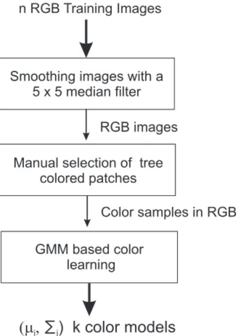
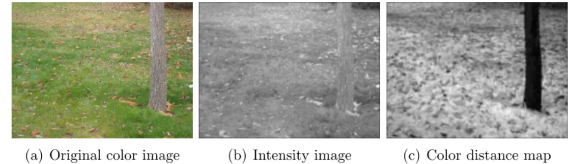
2.1 Example result of our tree trunks detection algorithm. Detected tree trunks: The base of each tree trunk is represented by a dia-mond and the edges of each tree truck are represented by overlaid thick lines. . . 16 2.2 Block diagram of our tree trunk detection algorithm. . . 17 2.3 Algorithm for tree color model learning based on GMM. . . 21 2.4 Color Transformation based on Mahalanobis distance. Dark

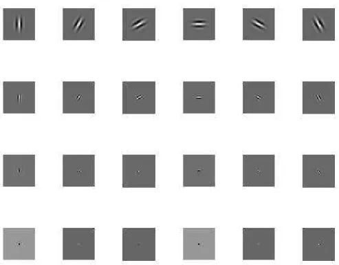
re-gions have a high probability (not formally) of having color values close to the learned tree color model. . . 25 2.5 Examples of Gabor wavelets in the spatial domain with six

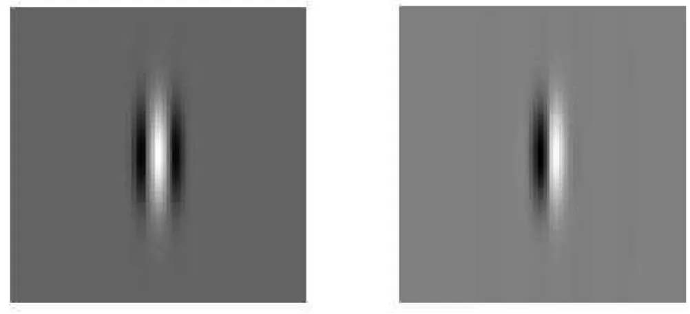
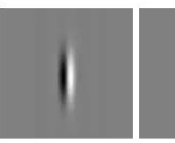
orien-tations and four different scales. . . 29 2.6 Intensity plot of the real (left) and imaginary (right) parts of a

vertically oriented 2-D Gabor filter in spatial domain with mid-gray values representing zero, darker values representing negative numbers and lighter values representing positive numbers. . . 31

2.7 Real (left) and imaginary (right) parts of a vertically oriented 2-D Gabor filter in the spatial domain. RGF consists of a central pos-itive lobe and two negative lobes and hence can be used to detect symmetric components. IGF consists of a single positive and a sin-gle negative lobe and hence can be used to detect antisymmetric components. . . 32 2.8 Examples of odd Gabor filter (IGFs) in the spatial domain with

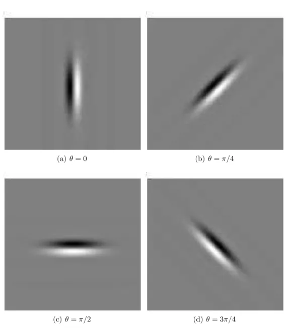
orientation θ = 0 and two different scales. . . 33 2.9 Examples of odd Gabor filters in the spatial domain with four

orientations and same scale. . . 34 2.10 The Gabor responses of the intensity image, shown in Figure 2.4.b

at four different orientations. . . 35 2.11 Algorithm for Gabor-based Edge Energy computation. . . 36 2.12 Example Gabor-based Edge Energy computation at vertical

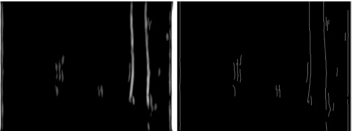
orien-tation for the image shown in Figure 2.4(a). Bright pixels indicate high response, while dark pixels indicate low response. . . 37 2.13 Example Edge Probability computation at vertical orientation for

the image shown in 2.4(a). . . 44 2.14 Example edge detection using the Modified Edge Flow method:

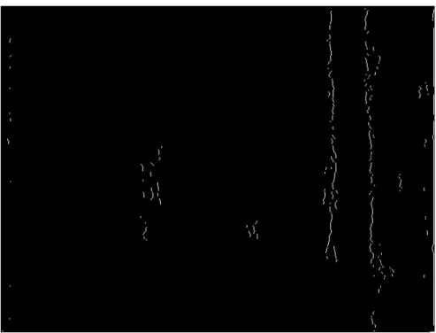
Quasi-vertical edges are detected from the image shown in 2.4(a). 45 2.15 Example Gabor-based edge detection: Quasi-vertical edges are

de-tected from the shown in Figure 2.4(a). . . 46 2.16 The DooG filter used in constructing edge classification masks.

The response of filter is positive at image locations with edges ori-ented at θ = 0 and negative at image locations with edges oriori-ented at θ = π . . . 48

2.17 Example edge classification masks construction. Bright pixel val-ues indicate the higher probability of finding an edge at orientation θ = 0 whereas darker pixel values indicate the higher probability of finding an edge at orientation θ = π and mid-gray pixel val-ues indicate the lower probability of finding an edge at orientation θ = 0 and θ = π, meaning that, indicate similar regions. . . 49 2.18 Labeled edge masks . . . 49 2.19 Construction of a suitable band of a potential pair. The two

pa-rameters ‘o’ and ‘w’ determine the size of the band. (a) shows the situation of being no occlusion, and (b) shows the situation of being occlusion. . . 50 2.20 Result of the edge linking (left) Before (right) After . . . 54 2.21 Analyzing directed angles (θsd and θds) for all possible joins enables

us to distinguish between co-linearity and co-circularity (a) All possible joins between S1 and S2, denoted as j1, j2, j3 and j4, (b) directed angles for the join j3 define a co-circularity relation since both of them are negative, (c) directed angles for the join j4 also define a co-circularity relation as both of them are positive, (d) directed angles for the join j2 define a co-linearity relation since θsd is negative and θds is positive, and finally (e) directed angles

for the join j1 also define a co-linearity relation as θsd is positive

and θds is negative. . . 57

2.22 Co-linearity vs Co-circularity (a) Co-linearity := θsd+ θds = 0, and

2.23 Analyzing a contour pair S1 and S2 for continuity. S1 is the source contour whereas S2 is the destination contour. The distance be-tween the end-points joining the source contour to the destination contour is denoted l. The directed angle θsd is defined as the angle

from the termination direction of the source contour to the connec-tion line. The directed angle θds is defined as the angle from the

connection line to the termination direction of the destination con-tour. The two termination directions (→) are the tangent vectors of the contours at the considered end-points. . . 59 2.24 Variables of continuity strength for all possible joins between S1

and S2 (a) S1 ⇒ source and S2 ⇒ destination, and (b) S2 ⇒ source and S1 ⇒ destination . . . 60 2.25 Construction of suitable bands for a potential pair. (a)

Construc-tion of suitable bands on each side of the edge contours, and (b) Construction of suitable bands on each side of the potential join. . 63 2.26 Effect of applying edge grouping based on continuity relation. Left:

before edge grouping, Right: after edge grouping . . . 65 2.27 Effect of applying Gabor-based edge pruning. . . 66 2.28 Proximity grouping, also known as co-curvilinearity on proximity 67 2.29 Analyzing a proximity relation between an edge contour pair S1

and S2. Endpoint distances are denoted as d1, d2, d3, and d4 and the projection distances are denoted as d5, d6, d7, and d8. . . 69 2.30 Construction of suitable bands for a potential edge contour. The

construction of suitable bands along each side of the contour and across the sides are described. . . 71 2.31 Effect of applying edge grouping based on proximity relation. Left:

2.32 Geometric attributes computed for each pair of straight contours S1 and S2 are demonstrated. The most important geometric at-tributes are: opening angle θoa, symmetry axis Ls, symmetry axis

segment Ss and the point of intersection Pc. . . 75 2.33 Different classes of overlapping are illustrated. In (a) the

projec-tions of the contours overlap and no one covers the other on the symmetry axis ⇒ overlapped. In (b) the projections of one con-tour completely covers the other on the symmetry axis ⇒ covered. In (c) the projections of the contours do not overlap each other on the symmetry axis ⇒ separated. . . 77 2.34 Different classes of corner junction are illustrated. In (a) the

posi-tion of Pc is between the end points of both contours ⇒ X-juncposi-tion corner type. In (b) the position of Pc is between the end points of only one contour ⇒ T-junction corner type. In (c) the posi-tion of Pc is not between the end points of any of the contours ⇒

L-junction corner type. . . . 78 2.35 Variables of symmetry strength . . . 82 2.36 Effect of applying edge grouping based on symmetry relation. Left:

before edge grouping, Right: after edge grouping . . . 87 2.37 Examples of our tree detection algorithm with each edge grouping

step: (a) Original color image, (b) Quasi-vertical edges detected with the Modified Edge Flow, (c) Result of edge linking, (d) Result of continuity-based edge grouping, (e) Result of Gabor-based edge pruning, (f) Result of proximity-based edge grouping, (g) Result of symmetry-based edge grouping, and (h) Final result. . . 88

3.1 Sample tree images in the heterogeneous dataset. . . . 90 3.2 Sample tree images in the homogeneous dataset. . . . 91

3.3 Sample tree trunks in the training dataset. . . . 92 3.4 Color distribution: (a) Tree-color cloud in RGB space, and (b)

Tree-colored vs. non-colored pixels. Red points represent tree-colored pixels and blue points represent non-tree pixels. . . 93 3.5 1-D histograms of tree vs. non-tree pixels with respect to

indi-vidual color components. Solid red and blue lines represent tree histograms and non-tree histograms, respectively. . . 94 3.6 Tree-color cloud in RGB space and Gaussian distribution

compo-nents which cover the cloud shown from two different views. Red points represent the cloud and alpha blended black tones ellipses represent Gaussian components. . . 96 3.7 The projections of the tree color model on the RG, RB and GB

subspaces, respectively. . . 97 3.8 Sample color distance images. Dark regions correspond to smallest

color distances. . . 98 3.9 Examples of clean and noisy tree trunks. . . . 99 3.10 Results of tree trunks detection methods under a cloudy and rainy

day. Although these tree trunks have different orientations, colors, textures and backgrounds, almost all of them are correctly detected by our methods. . . 103 3.11 Results of tree trunks detection methods under a sunny day.

Al-though these tree trunks have different orientations, colors, tex-tures and backgrounds, almost all of them are correctly detected by our methods. . . 104 3.12 Some examples of falsely detected tree trunks. . . 105 3.13 Some results of our proposed method for detecting tree trunks with

3.14 Results of tree trunks detection methods in forested outdoor envi-ronment under different weather conditions. Although these tree trunks have non-homogeneity in bark textures and colors, almost all of them are correctly detected by our method. . . 109 3.15 Results of tree trunks detection methods in cluttered forested

out-door environment under different weather conditions. Although these tree trunks have non-homogeneity in bark textures and col-ors, and complicated background conditions, almost all of them are correctly detected by our method. . . 110

2.1 Continuity Parameters . . . 62

2.2 Continuity consistency . . . 64

2.3 Confirmation of continuities . . . 64

2.4 Confirmation of proximities . . . 70

2.5 Color Symmetry Consistency . . . 80

2.6 Intensity Symmetry Consistency . . . 80

2.7 Confirmation of symmetries . . . 80

3.1 Performance comparisons among three different methods for the heterogeneous dataset. . . 100

3.2 Comparison of correctly detected tree trunks of our methods and Asmar et al. [1] for the heterogeneous dataset in terms of ‘clean’ and ‘noisy’. . . 101

3.3 Performance comparisons among three different methods for the homogeneous dataset. . . 107 3.4 Comparison of correctly detected tree trunks of our methods and

Asmar’s for the homogeneous dataset in terms of ‘clean’ and ‘noisy’.107

Introduction

Today, robotic systems are used instead of humans in many areas such as the au-tomotive and manufacturing industry for lifting heavy objects [2–5], cutting and shaping parts, assembling machinery, inspection of manufactured parts, the mil-itary for warfare [2, 5–10], autonomous soldiers, tanks, weapons systems, planes, fighter jets and bombers, unmanned autonomous helicopters, investigation of haz-ardous and dangerous environments, space and earth exploration [2, 5, 7, 11–13], transportation [2, 14, 15] and medical applications [16] to perform tasks which are too dirty, dangerous or dull for humans. To perform such tasks, robots need to be able to move by themselves, that is, ‘autonomously’. An autonomous robot is a robot which can move by itself, either on the ground or in the air/space or underwater without human guidance [5]. This can be achieved by equipping these systems with various on-board sensors and computational resources in order to guide their motion.

An important application of autonomous robotic systems is to travel where people cannot go, or where hazards for human presence are too big (e.g. explo-ration of other planets where the surface has no air, water or resources to support human life [11, 12] or exploration of underwater life where pressure, light, currents or other factors limit human exploration [13]). Such applications require percep-tion of the environment through sensors. Processing of sensor outputs helps build useful representations of the unknown environment, which can then be used for

navigating and controlling the system.

Autonomous robot navigation is known as the ability of a robot to move from

one location to another without continuous human guidance, while avoiding ob-stacles in unstructured environments based on its sensor information [17]. In order for a mobile robot to successfully perform a navigation task, it often re-quires to answer the following questions: “Where am I now?”, “Where am I going?”, and “How should I reach there?”. These questions are formally known as robot localization (pose estimation), goal specification, and path planning, re-spectively. Autonomous robot navigation in an unknown environment is an open research problem that many researchers have addressed over the years. Related studies show that among most successful navigation algorithms are the ones that are based on robot localization [18]. Thus, the ability of a robot to localize itself is critical to its autonomous operation and navigation.

Robot localization is defined as the process of determining the exact position

of a robot within its environment and is a fundamental problem in autonomous robot applications [18]. Robotic systems can rely on various types of sensors to gain information about the environment and their own position. These sensors include infrared sensors, ultrasound sensors, laser range scanners, global position-ing system (GPS), inertial measurement units (IMU) and cameras.

Traditionally, information from wheel, GPS and IMU sensors have been used to obtain a robot’s position and speed, and possibly its trajectory in a given map of its environment [19]. Despite the popularity and usefulness of above sensing techniques, they suffer from drift, low resolution, high cost or size problems, limiting their applicability. For example, wheel odometry performance degrades in presence of wheel slippage and GPS suffers from low resolution and low update rates. GPS outages are also common in some settings, such as urban environments or forests. Similarly, IMU sensors are expensive, prone too high noise levels especially at low speeds and their accuracy is affected due to the need for double integration over time if position estimates are required [20–22].

In contrast, absolute positioning and localization are still possible by per-forming map-based robot localization, also known as simultaneous localization

and mapping (SLAM). There has been extensive research into the SLAM

prob-lem over the past two decades (see [23, 24] for a comprehensive survey). In the following section, we will give a brief overview about SLAM.

1.1

SLAM: An overview

SLAM is a process by which an autonomous robot can build a map of an environ-ment and at the same time, use this map to estimate its location [25]. SLAM is a suitable solution for autonomous robot navigation in outdoor settings when GPSs may be unavailable or unreliable. The processes of localization and mapping are strongly coupled. To determine the robot’s location, the robot must have a map, but to build the map, the robot must also first know its location. This strong coupling is one of the factors that makes SLAM difficult.

In SLAM, the robot has to recognize salient features or landmarks present in the environment to build its navigation map. These are detected by using external sensors (e.g. laser range sensor, sonar sensor and camera) that provide information relative to the position of the robot. Initially, both the map and the robot position are unknown, the robot has a known kinematic model and it is moving through the unknown environment populated with landmarks [26]. Consequently, a simultaneous estimate of both robot and landmark locations is required. The two main problematic issues in SLAM are what landmarks to look for and how to detect them.

1.1.1

Landmark Selection

Navigation maps are built via using landmarks. Consequently, in order to per-form SLAM, landmarks have to be detected in the robot’s environment. A key characteristic for a good landmark is that it can be reliably detected [27]. This means that the robot should be able to detect it over several frames. Addition-ally, the same landmark should be detectable when the same area is visited again,

meaning that detection has to be stable under viewpoint changes. Landmarks can be natural (like roof or tree edges) or artificial (like reflective stripes, active beacons or transmitters) having a fixed and known geometric properties [28].

Detecting landmarks is a difficult task. For this reason, in most implemen-tations, SLAM landmarks have been restricted to artificial beacons with known geometric properties [29–31]. Natural landmark-based methods for autonomous localization have become increasingly popular [1, 28] as they do not require any infrastructure or other external information. Such methods require that natural landmarks can be robustly detected in sensor data, that the localization algo-rithm can reliably associate landmarks from one sensor observation to the next, and that the method can overcome problems of occlusion, ambiguity and noise inherent in observation data [28].

As pointed out by [32], there is a need for methods which enable a robot to autonomously choose landmarks. A good method should pick landmarks which are best suited for the environment the robot wishes to map. For example, in in-door environments, features such as walls (line-segments), corners (diffuse points) or doorways (range discontinuities) are used as landmarks. They can easily be determined and provide robots with good structure and organization for image processing tasks. In outdoor environments however, similar simple features are sparse and infrequently observed. Thus, outdoor environments tend to be un-structured, inhibiting the use of the same indoor algorithms. In unstructured or natural environments, it is difficult to specify a generic feature that could be present in all environments. For instance, features tracked in an off-road en-vironment would be different than those tracked in an urban location or in an outdoor park or in an underwater setting. In such environments, the knowledge of the environment could significantly reduce the search space of candidate land-marks. The identified environment dictates what landmarks should be selected for SLAM [33]. This is, however beyond the scope of this thesis, which focuses on the problem of object detection as natural landmarks for SLAM. In this context, our experimental setting (a sparsely forested outdoor environment) and land-marks (tree trunks) are chosen beforehand and the problem we focus on is that of detecting these landmarks.

1.1.2

Sensor Selection

In order to achieve accurate localization of the robot, the robot must be equipped with a sensory system capable of taking measurements of the relative location between landmarks and the robot itself. These sensors are exteroceptive sensors such as laser range finders (LRFs), sonar sensors or cameras to localize landmarks around the robot and subsequently improve the robot pose prediction [24].

One of the most important factors that determines the performance of SLAM algorithms is naturally the accuracy of the relative external sensor. For example, in the case of sonar or laser sensors, this is determined by the range and bearing errors when observing a feature or landmark [26]. Additional sensory sources, such as, compasses, infrared technology and GPS may also be used to better perceive robot state and the outside world [23]. However, all these sensors carry certain errors, often referred to as measurement noise, and also have several range limitations making necessary to navigate through the environment.

Another important issue for SLAM is data association, defined as the problem of recognizing a previously viewed landmark and maintaining correspondence be-tween a measurement and a landmark. In this context, there has been significant research related to SLAM using various kinds of sensors [34–43]. Many of these mapping systems rely on Laser Range Finders (LRFs) or sonars.

LRFs are accurate active sensors but they are slow, expensive and they can be bulky. Their most common form operates on the time of flight principle by sending a laser pulse in a narrow beam towards the object and measuring the time taken by the pulse to be reflected off the target and returned to the sender. Sonar-based systems are fast and cheap but usually very crude. They provide measurements and recognition capability similar to vision, but they do not provide appearance data. In summary, due to their high cost, problems with speed, accuracy and safety, active sensor-based SLAM methods have limitations in practical applications. Also, its dependence on inertial sensors implies that a small error can have large effects on later position estimates [23].

While traditionally LRFs have been primarily used as exteroceptive sensors for outdoor SLAM, vision sensors, especially cameras, received increasingly more attention [44–49] due to their low cost, low power consumption, passive sensing, compactness, light-weight and capacity to providing textual information. Fur-thermore, cameras provide more information than LRFs or sonars.

As mentioned before, laser range sensors or sonars have been traditionally used to detect landmarks. However, landmarks that they can detect are limited in complexity due to the low bandwidth information these sensors can provide. Consequently, in this thesis, we use a camera as our exteroceptive sensor to perform detection of landmarks.

1.2

Problem Statement

The work in this thesis addresses the problem of detecting tree trunks in images of cluttered outdoor environments for the purpose of using them as landmarks for visual-SLAM-based autonomous robot localization using a single digital camera as a sensor. The problem of detecting tree trunks can be formulated as follows: Given an arbitrary image, determine whether or not there are any tree trunks in the image, and if present, report the base location and extent/size of each tree trunk. This problem is rather challenging for the following reasons:

• Image conditions such as lighting (spectra, source distribution and inten-sity) and camera characteristics (sensor response, lenses) may substantially change the appearance of a tree trunk.

• Different cameras may produce different appearance information even for the same tree under the same pose and illumination.

• Varying viewpoint may change the appearance of a tree trunk.

• Trees have a high degree of variability in size, color, brightness and texture even for trees within the same species.

• Different types of trees will have different appearances depending on the texture of the bark, the smoothness of the trunk, the density of the branches, shadow, brightness and color.

• Some potential background objects such as rocks and sand share similar texture and color information with trees. Nevertheless, a common feature of all tree trunks is their quasi-vertical and symmetric structure. Even as such, some potential background objects such as buildings, dustbins, rods, roads or traffic signs and pipes shares similar structural information with trees.

• Tree trunks can be of any intensity in the image, from very dark to very light. Also, some tree trunks’ intensity is very close to background objects such as leaves, glass and road. Moreover, when the image resolution is low, not many details are visible.

• Tree trunks may be partially occluded by the environment in the images, mostly undergrowth.

We need to address all these issues to obtain a reasonably good tree trunk detec-tion system.

1.3

Existing Work on Tree Detection

In this section, we provide some background information on various techniques that have been suggested to detect trees in images. Maeyama et al. [50] proposes a method that estimates the position of a mobile robot using trees as landmarks in an outdoor environment. In this method, both sonar and vision sensors used to detect trees in images. The tree detection algorithm they propose is based on two assumptions: First, they assume that the structure of a tree in an image is vertical, meaning that both sides of a tree in an image are vertical edges. As a result of this, a differential operator in x-direction is applied to an image to obtain the vertical edges in the image. Their other assumption is that the tree

constitutes an image area whose intensity values are darker than the background and uniform in shading. As a result of this, the differential values on the left side edges of trees trunk are negative, while those on the right are positive. In addition to this, distance measurements obtained by a sonar sensor are used to make an estimate of the position of central axes of trees in images. Those positions are then used as landmarks to estimate the robot’s position in the environment. The main drawbacks of this method are its assumptions on the homogeneous appearance of trees and the lower intensity values on the tree. Consequently, this method would not work well for images with a wide variety of illumination, non-homogeneity in bark texture and the background sharing similar appearance and/or structure information with trees in the foreground.

Asmar et al. [33] proposes a method that detects trees in an outdoor environ-ment using local descriptors. This method involves the construction of a training set in a weakly supervised manner. The training set consists of both positive and negative images; positive images are ones which contain trees while negative images are those which contain only background objects. In the training phase, a Difference of Gaussian filter is applied to images at different scales in order to de-tect interest points inside the image and those points are represented using scale invariant local descriptors. Similar descriptors are clustered together and those clusters are used as object classifiers. Object classifiers are then ranked according to their classification likelihood by the purpose of reducing mismatch probabil-ities. As a result, descriptors representing trees receive high ranks while those representing background receive low ranks. When a query image is encountered, descriptors are then used to match with existing clusters. The rank information is used to classify it as a tree or a background object. An important property of object detection using local descriptor is its repeatability. Different trees present a large amount of variability in their appearance and thus, none of the internal features of one tree are probably to be found on another tree. The only common characteristic between tree trunks is their quasi-vertical and symmetric structure. Under such conditions, it is difficult to correctly detect trees in images using lo-cal descriptors. Another problem is that interest points or regions need to be distinctive from the rest of the image. However the backgrounds of tree images

(e.g. glass, sand, rock, etc.) share similar color and texture signatures with the trees in the image.

Huertas et al. [51] proposes a stereo-based tree traversability algorithm that estimates the locations and diameters of trees in the scene by detecting portions of tree trunks using their vertical structural information. They assume that por-tions of tree trunk (called as tree trunks fragments) are discernable from the background, meaning that portions of tree trunk appear either brighter or darker than the background, and thus the boundaries that delineate portions of the trunk are detectable and also have opposite contrast. First, their proposed method de-tects edges that belong in contours having vertical or near vertical directions by applying edge detection in horizontal direction and contour extraction. Then, the method uses edge contrast polarity and stereo range data to match pairs of edges of opposing contrast along the horizontal direction that correspond to the bound-aries of individual potential tree trunks fragments. Subsequently, the diameter of each tree trunk fragment is estimated based on stereo range data and estimated diameters are then used to construct a tree traversability image. Their proposed method focuses on detecting tree trunk fragments rather than tree trunks. This means that the system does not attempt to group tree trunk fragments to form tree trunks. Hence, multiple fragments on a single tree trunk can be observed. The main disadvantage of this method is their assumption on intensity values on trees. Only tree trunk fragments that appear darker or brighter than the back-ground can be detected by this method. Consequently, this method is not very robust under varying illumination conditions and environmental settings.

Teng et al. [52] proposes an algorithm for tree segmentation. They consider only trees having clear tree trunk (homogeneity in bark texture and color ap-pearance) and leaf region. In this algorithm, trunk and leaf regions of a tree are individually identified and the trunk structure of a tree is also extracted. Their proposed algorithm consists of three stages: preliminary segmentation, trunk structure extraction and leaf region identification. In preliminary segmentation stage, the image is partitioned into several regions using EM algorithm and an energy function is formulated according to the color, position, and direction of the segmented regions. Then, non-trunk regions are removed using a systematic

method to correctly extract the trunk structure and after that, the trunk struc-ture is extracted by minimizing an energy function. After obtaining the trunk structure, leaf regions are then easily extracted by finding consistent regions lo-cated above the trunk regions. In our case, most of images do not contain leaf regions. However, in this method, tree trunk regions are determined based on the locations of leaf regions, meaning that although, the regions that belong tree trunks are classified as non-tree trunk regions if they do not have leaf regions above them. Additionally, those locations are used to reduce the effect of back-ground regions similar to trees and the locations of trunk regions are utilized to eliminate the effect of background regions similar to leafs. Consequently, for these reasons, this method is not suitable for our case.

Asmar et al. [1] also proposes a method to detect tree trunks in images for the sake of using them as landmarks for visual SLAM. In this method, a tree trunk is defined as follows: “A tree trunk is a combination of symmetric and continuous lines, its base is connected to the ground, its direction is predominantly vertical, and the value of its aspect ratio is constrained and this definition is used as a basis for the detection of tree trunks.” Their proposed algorithm is based on the vertical nature of the tree trunks and location of the tree trunks base. In this algorithm, edges dominant in the quasi-vertical direction are obtained first by applying a Canny edge detection algorithm in the vertical direction to the input image. Vertically dominant edges are then perceptually organized into continuous and symmetric lines, and are subsequently grouped into tree landmarks by minimizing the entropy of the image and removing non-tree lines using the location of the tree trunk base. The Ground-Sky (G-S) separation line, obtained by applying the Canny edge detection algorithm in the horizontal direction to the input image, is located in each image and used to estimate the position of the tree trunk base. Our proposed solution is inspired from this method and substantially improves on performance when the intensity of tree trunk regions is similar to the background. In such case, vertical edges are not obtained accurately with this method (i.e, some of the tree edges are not detected or the location of tree edges are not obtained correctly). In addition, this method does not distinguish well trees from background objects that have similar structure and appearance because

of using only intensity information. Consequently, the main drawback of this method is using only intensity information to obtain edges in an image. However, our proposed method is very close in spirit to this work and improves on its performance under varying illumination, texture and background conditions.

Ali et al. [53] proposes a classification based tree detection and distance mea-surement method for autonomous vehicle navigation in forest environments. This method consists of three parts: the training step, the pixel/block classification step and the segmentation and distance measurement step. In the training step, each training image is divided into small non-overlapping blocks and each block is classified as either background (leaves, snow, bushes with snow, and leaves with snow) or foreground objects (brown and black tree trunks) manually. Then, both color (color histogram or mean or standard deviation of color) and texture (Co-occurrence matrix, Gabor filters, or Local Binary Patterns-LBP) features are computed from each block and stored in vector form. Subsequently, feature vectors are obtained by using only color, only texture or the fusion of both by simply concatenating both type of features into a single feature vector without considering their weights. After that, feature vectors are classified using Artificial Neural Networks (ANN) or K-Nearest Neighbor (kNN) classification algorithm. In the pixel/block classification step, test image is also divided into small blocks and feature vectors are extracted from each small block. Then, those feature vectors are fed into the selected classifier (ANN or kNN) to classify each block as tree or background. In the segmentation and distance step, a binary image based on the classification results is constructed by assigning white color to tree blocks and black color to others in an image and the distance between the base of the tree and the tire of vehicle is estimated by using a simple heuristic method based on pixel ratio and the width of the tire as a reference. The main draw-back of this method is that it only detects trees in a known environment under known climate conditions. Their background classes only consist of leaves, snow, bushes with snow, and leaves with snow. Therefore, this method is not suitable for our case since we try to detect trees in cluttered outdoor environment under unknown climate conditions. Moreover, the performance of this method is based on the classification performance of small blocks and this situation might cause

problems such as some trees not being recognized.

1.4

Our Contributions

This thesis presents a novel method for detecting tree trunks in cluttered out-door environments using a single digital camera. Our method incorporates both appearance and structure information in an image towards robust of detection of tree trunks. The tree trunk structure is defined as follows, inspired from [1]: ‘A tree trunk is a combination of symmetric and continuous edges, its direction is predominantly vertical, and the value of its aspect ratio is constrained.” This definition is used as a basis for our solution. In our method, edge strengths of images are first obtained using intensity, color and texture information. Subse-quently, dominant edges in the vertical direction are detected using a variant of the Edge Flow segmentation algorithm [54, 55] or complementary Gabor-based edge detection algorithm. These dominant edges are then grouped into poten-tial tree trunks using the integration of perceptual organization properties and regional attributes.

The major contributions of this thesis are as follows:

• Due to the difficulties explained in Section 1.2, using only appearance in-formation or structure inin-formation cannot be expected to produce good results. Therefore, we use an integration of both appearance (i.e. regional attributes) and structure information (i.e. perceptual organization) to de-tect tree trunks in cluttered outdoor environments.

• We use a specifically tuned color filter as a pre-processing step. We trans-form an image into color distance map (CDM) using a pre-computed tree color probability distribution. The CDM is later used as color information during edge detection and grouping. Using the CDM makes the procedure simple because it reduces the image to a single channel of distance values and informative because it implicitly uses color information while retaining structural information that is present in the image.

• We apply odd Gabor filters bank to both intensity image and CDM to compute the edge strengths at different orientations of an image. By this way, we use intensity, color and texture information during edge detection. • In the original Edge Flow method [54, 55], after obtaining the edge energies and the corresponding probabilities from different image attributes, they are combined together to form a single edge flow field for boundary detection. In our case, instead of handling each image attributes separately, we consider all image attributes simultaneously. Moreover, instead of using the gradient of the smoothed image for computing edge energies, we use the Gabor representations of the image.

• We present a Gabor-based edge detection method that uses the edge strength of the image at the vertical orientation to detect the vertical edges in the image.

• During edge grouping process, we consider both perceptual organization tools and regional information. Using regional information enables us to measure the consistency and accuracy of predicted edge pairs with image structure. In other words, a geometric relationship defined between two edge contours is verified if associated regional attributes are in agreement. We use regional properties along each edge contour and in pixels surround-ing each edge contour to verify the predicted pairs. We construct edge classification masks, that indicates whether a pixel is a part of the desirable structure or not, for the sake of using them as regional information. Also, we use CDM as regional information.

• In contrast to [1], in addition to continuity and symmetry, we use proximity, parallelism and co-curvilinearity properties of edges and regional informa-tion during edge grouping process. Moreover, in addiinforma-tion to intensity, we use color and texture information during edge detection process.

The effectiveness of our proposed algorithm for detecting trees is then evaluated on an extensive collection of outdoor images containing trees.

1.5

Organization of the Thesis

The rest of the thesis is organized as follows: Chapter 2 gives the details of the proposed tree trunks detection system, which integrates perceptual organi-zation capabilities with low-level image features. Experimental results are then presented in Chapter 3 to demonstrate the robustness of the method under a variety of environmental conditions and experimental results are then discussed. Moreover, the accuracy of our proposed method is compared to the method pro-posed by Asmar et al. [1] and comparison results are also discussed in Chapter 3. Chapter 4 concludes with a summary of our proposed method and introduces the focus of our future research.

Moreover, relevant approaches for object detection are discussed in Appendix A. Besides, we discuss potential solutions and emphasize which one is suitable for our case.

Detection and Extraction of Tree

Trunks

In this chapter, we describe our algorithm for detecting and extracting tree trunks in color images of outdoor scenes. To make this method quick and easily under-standable, we first briefly explain the algorithm and then, discuss each step in detail.

2.1

Motivation and Algorithm Overview

Our problem can be defined as detecting tree trunks for the purpose of using them as natural landmarks for autonomous robot localization in cluttered outdoor environments using a single digital camera as a sensor. The task of detecting tree trunks is to determine whether or not there are any tree trunks in a given image, and if present, to localize each tree trunk (See Figure 2.1). In this work, inspired from [1], we define tree trunks as follows: “A tree trunk is a combination of symmetric and continuous edges with a predominantly vertical orientation, and having a limited range of possible aspect ratios.” Our problem is hence reduced to detecting quasi-vertical edges in images using both color and intensity as well as texture information and then, grouping detected edges into potential tree trunks

Figure 2.1: Example result of our tree trunks detection algorithm. Detected tree trunks: The base of each tree trunk is represented by a diamond and the edges of each tree truck are represented by overlaid thick lines.

by using the integration of both geometric relationships and regional attributes. To this end, we propose a novel edge-based segmentation method to effi-ciently extract tree trunks from color images of outdoor scenes with wide range of tree-color variations, varying illumination conditions, shadows, non-homogeneous bark texture, different tree orientations and complex background. The proposed method consists of two steps: learning of tree colors and detecting of tree trunks. In the learning step, based on a set of sample pixels extracted from a wide variety of trees having different color tones and captured in different lighting and illu-mination conditions, the distribution of tree colors is modeled using a Gaussian mixture model.

Once the color model is learned, Figure 2.2 summarizes the general flow of our tree trunk detection algorithm with each one of the six steps briefly explained below:

1. Pre-processing: We collect tree images from different kinds of trees under different illumination and weather conditions. Those images are represented

Figure 2.2: Block diagram of our tree trunk detection algorithm.

in the RGB color space and depending on the selection of color space, the images are converted into the selected color space such as HSV, NRGB, YCbCr or gray-scale. If desired, those images are resized after smoothing with a Gaussian filter at appropriate scale to speed up the tree detection procedure. In our experiments, we have observed that images with 640 × 480 pixels in resolution still preserves sufficient color, intensity and texture information.

2. Tree-colored pixels detection: The original image is transformed into a tree-color distance image. Tree-tree-colored pixels in the image are detected by using the tree color probability distribution computed during the learning phase, modeled using a Gaussian mixture model (GMM).

3. Obtaining intensity image: Ideally, the background in the image has dif-ferent intensity with the trees in the foreground so we also transform the original image into an intensity image. After that, the intensity image is smoothed using an Anisotropic diffusion filter [56]. This is necessary step

since most real images are noisy and have corrupted data. Moreover, elim-inating noisy pixels improves the efficiency and accuracy of the rest of the proposed algorithm. Finally, the resulting image is normalized to the range [0, 1].

4. Computation of Edge energies: Edge energies of the image at different ori-entations and scales are computed by filtering both intensity image and tree-color distance images with a bank of odd Gabor filters. These edge energies indicate strengths of the intensity, texture and color changes. 5. Edge detection: Quasi-vertical edges in the image are detected by using a

modified version of the Edge Flow method or using complementary Gabor-based edge detection method.

6. Edge Grouping: Detected edges are grouped into potential tree trunks by using the integration of a variety of geometrical properties of edges such as curvilinearity, continuity, and symmetry and regional attributes such as color and edge classification masks.

In the following sections, we will describe the details of each of these components.

2.2

Color Learning and Transformation

Color is a perceptual phenomenon related to human response to different wave-lengths in the visible electromagnetic spectrum [57]. Human eye can discern thousands of color shades and intensities while only two-dozen shades of gray color, and responses more quickly and accurately to what is happening in a scene if it is in color [58]. Color is helpful in making many objects “stand out” when they would be subdued or even hidden in a gray-level (monochrome) image [59]. Compared to monochrome image, a color image provides in addition to inten-sity, the additional information (chromatic information) about the objects and the scenes. Using chromatic information allows to overcome problems which are difficult to solve images for which only intensity is available [59]. Therefore, color

is useful or even necessary for pattern recognition and computer vision systems, particularly important to detect or recognize the objects that can be easily cate-gorized in color distribution [59, 60].

In computer vision, researchers have attempted to use color information in many applications such as image or scene segmentation [59, 61, 62], object detec-tion or recognidetec-tion [63–68], detecdetec-tion of certain colored regions in images [64, 69– 73] and edge detection [74–77]. In our case, color information is mainly used to detect the certain colored regions (tree-colored patches) in images.

In this thesis, one of our novel contributions is the use of color information to distinguish trees from the background. Color is highly robust to scale and orientation changes, and also not effected much by the motion of other objects [59, 60]. However, color information is influenced by illumination conditions and differs from tree to tree. In addition, different cameras may record colors differ-ently. In order to address all these problems, and to effectively distinguish trees from background objects based on color information, we need a reliable color model. This model must accommodate trees of different color tones and different illumination and lighting conditions.

Both non-parametric and parametric methods are used for modeling color distribution in the literature. The key idea of the non-parametric color modeling methods is to estimate color distribution from the training data without deriving an explicit model of the color distribution. Non-parametric techniques include piecewise linear decision boundaries (such as thresholds on color features) [78, 79], and Bayesian classifier with the histogram technique [64, 80]. In case of parametric modeling, on the other hand, a predefined statistical model is selected to model the color distribution. Parametric techniques include modeling of color distributions using unimodal Gaussians or mixtures of Gaussians [62, 70, 72, 81– 83] or multiple Gaussian components [65] or an elliptic boundary model [84]. Besides, nonlinear models such as multilayer perceptrons are used to model color distribution[85].

Parametric modeling is more sensitive to the choice of color space than the non-parametric modeling because of the effect of the shape of color distribution.

On the other hand, non-parametric models are not only independent of the shape of color distribution, but also they are faster in training and testing. However, non-parametric techniques require a large amount of training data and thus, more storage requirements and there is no way to generalize the training data, so they may not be practical in many cases [86]. On the other hand, Gaussian mod-els can generalize well with less training dataset and also have very less storage requirements. The performance of Gaussian models directly depends on the rep-resentativeness of the training dataset, which is going to be more compact for certain applications (such as skin color detection) in color model representation. Therefore, in this work, Gaussian models will be discussed.

Our algorithm assumes that tree trunks have families of roughly similar colors. Hence, we propose to use a color distance map (CDM), where distance value of each pixel gives an idea of how close the pixel color resembles a tree trunk. This procedure is efficient since it reduces the image to a single channel of distance values and informative since it retains the structure of the image. The proposed method constructs the CDM based on a tree color model: The input image is transformed into a CDM (tree-color distance image) such that the value of each pixel shows the possibility that the pixel belongs one of previously learned tree color classes, calculated based on the Mahalanobis distance between the pixel‘s color value and the tree color model.

In summary, our method requires the selection of a suitable color space, a reliable color model to represent the distribution of tree colors and a suitable similarity criteria to distinguish tree-regions from non-tree regions based on color information. Our method consists of two steps: color learning and color trans-formation which are described in detail in the following sections.

2.2.1

Learning Tree Color Models

Our tree color model learning algorithm involves three steps, shown in Figure 2.3 and briefly explained below:

Figure 2.3: Algorithm for tree color model learning based on GMM. 1. Collection of the training dataset: The training dataset for our algorithm

consists of RGB images including different kinds of trees under different illumination and lighting conditions.

2. Selection of color samples: Objects in real-world images are rarely smooth in terms of color. With regard to trees, a tree is never completely homo-geneous in terms of color. Image smoothing may help to negate some of this noisy information, which would otherwise be garnered from an image and can impact on further image processing steps. In order to eliminate image noise, training images are smoothed with a 5 × 5 median filter [87– 89]. Then, tree-colored patches are manually selected from each image to obtain a large enough set of pixels with desired range of colors.

3. Color space selection: A suitable color space must be chosen to represent color models for tree trunks. Tree pixels are then converted to the selected color space. Different color spaces, namely YCbCr [59, 62, 65, 66, 90–92], HSV [59, 67, 73, 74, 90–95] and RGB [59, 64, 69, 90, 92] will be considered. The HSV seems to be a good alternative since it is compatible with the human color perception, but HSV family presents lower reliability when the

scenes are complex and they contain similar colors such as wood textures [96]. Moreover during the image acquisition, camera provides RGB image directly, so choice between RGB and YCbCr arises here.

RGB components vary with the changes in the lighting conditions, thus color detection may fail if the lighting condition changes. YCbCr is a linear transformation of RGB so that it produces nearly same results with RGB. Hence, CbCr subspace is considered first for color detection. According to our experiments, CbCr produces quite better results than RGB but color transformation is required. For example, each image of size 640 × 480 pixels requires (640x480 =) 307200 transformations. In order to avoid such a huge amount of heavy calculations, and since most cameras provide RGB images directly and with respect to our observations, RGB is the best alternative in this thesis. Therefore, RGB color space is used here to represent color distribution of tree-colored samples.

4. Learning of tree color model parameters: We use a Gaussian mixture model to model the distribution of the tree colors since closed form estimates of their parameters can be computed using the Expectation-Maximization (EM) algorithm.

In the RGB color space, we model the distribution of tree colors using a Gaus-sian mixture model (GMM). To estimate the parameters of the GausGaus-sian mixture model, we use the standard Expectation-Maximization (EM) algorithm. The al-gorithm begins by making an initial guess for the parameters of the Gaussian mixture model using the k-means algorithm. Then, the EM algorithm is run on the training data using a stopping criterion that checks whether the change in negative log-likelihood between two iterations, which can be regarded as an error function, is less than a given threshold. In other words, given the training data D = {x1, . . . , xn}, the change in error function is computed by using the Equation

2.1 [82]: ∆t+1 = Et+1_{− E}t_{= −} n X i=1 ln(p t+1_(x i) pt_(x i) ) , (2.1)

where pt+1_{(X) denotes the probability density evaluated using ‘new’ values for the}

values. By setting the derivatives of ∆t+1 _{to zero, we obtain the following update}

equations for the parameters of mixture model [82]: µt+1 j = Pn i=1pt(j|xi)xi Pn i=1pt(j|xi) (2.2) Σt+1_j = Pn i=1pt(j|xi)(xi− µt+1j )(xi − µt+1j )T Pn i=1pt(j|xi) (2.3) αt+1j = Pn i=1pt(j|xi) n , (2.4) where pt (j|xi) = pt_(x i|j)αtj Pk m=1αtmpt(xi|m) (2.5) .

The number of components in the mixture k can be either supplied by the user or chosen using the Minimum Description Length (MDL) Principle [97] that tries to find a compromise between model complexity and the complexity of the data approximation. Under MDL, the best model M is the one that minimizes the sum of the model’s complexity (κM

2 log n, where κM is the number of free

parameters in model M ) and the efficiency of the description of the training data with respect to that model (− log p(D|M)). For a Gaussian mixture model with k components, the number of free parameters becomes κM = (k −1)+kd+k(d(d+1)₂ )

and the best k∗ _{can be found as}

k∗ = arg min k [κM 2 log n − n X i=1 log( k X j=1 αjp(xi|j))] (2.6)

2.2.2

Computing the Color Distance Map

Using the tree color model computed using the algorithm described above, we transform color images into tree-color distance images, where the gray-level in-tensity of each pixel represents its possibility of belonging to a tree color class. More formally, each pixel value represents the minimum Mahalanobis distance from its color to the tree color model clusters. Hence, tree-color distance image can be considered as a color distance map, showing how far the color of each pixel is from the learned model.

We define Color Distance (CD) as the Mahalanobis distance between the color of a pixel and a tree color cluster. The CD is naturally related to the probability (not formally) of a color to be considered as tree color. The lower the CD is, the higher the probability of that pixel being a part of a tree trunk is. The Color

Distance Map (CDM) is then defined as a gray-scale image obtained from a color

image by assigning to each pixel in the image, the Mahalanobis distance from the color value of the pixel to the ‘closest’ tree color cluster. Some properties of the CDM are listed below:

1. The CDM represents the likelihood (not formally) of each pixel in the image being a part of a tree trunk regardless of the number of tree clusters specified by the color model.

2. The CDM provides both color and shape information. Despite being a single channel image, the CDM still retains enough shape and color information because CDs represents distance in the color space.

The distribution of the tree colors is modeled using a GMM in the RGB color space and hence, the centroid of each model cluster is determined by the mean vector µj and its shape is determined by the covariance matrix Σj. Let

c = [R, G, B]T _{be a color pixel located at coordinate (x, y) of a color image.}

The CDM of this pixel can be computed as CDM (x, y) := arg min

j

CD(c, µj, Σj) where j = 1, . . . , k (2.7)

where CD(c, µj, Σj) is the Mahalanobis distance from the pixel c to the j’th

model cluster, defined as

CD(c, µj, Σj) := (c − µj)T Σ−1j (c − µj) (2.8)

Here, taking the smallest CD ensures that the distance to the closer cluster is chosen. Thus, a single CDM represents all clusters included in the tree color model. CDM values represent the probability (not formally) of each pixel to be taken as a tree pixel.

Due to large variations in lighting and illumination conditions and the exis-tence of background objects similar in color to trees, there are usually isolated groups of “noise” pixels in the resulting CDM. These regions typically have a size of a few pixels and can be eliminated using morphological opening and closing operators. Opening suppresses bright details smaler than the structuring ele-ment and closing suppresses dark details smaller than the structuring eleele-ment [88, 89, 98, 99]. We apply sequential opening and closing operations using 3 × 3 square structuring elements to eliminate these “noise” regions. Opening elimi-nates small bumps that are connected to tree regions and closing gets rid of small blobs within tree regions. After that, we apply an Anisotropic diffusion filter [56] to the resulting CDM. Eliminating “noise” regions in this manner improves the efficiency and accuracy of the rest of the proposed algorithm. Finally, the resulting CDM is normalized to the range [0, 1].

A sample color image and its resulting color distance map are shown in Figure 2.4.

(a) Original color image (b) Intensity image (c) Color distance map

Figure 2.4: Color Transformation based on Mahalanobis distance. Dark regions have a high probability (not formally) of having color values close to the learned tree color model.

2.3

Gabor-based Edge Energy Computation

In recent years, the Gabor filters have been received considerable attention in image processing applications especially texture segmentation and analysis [100– 104]. Texture segmentation requires both simultaneous measurements in spatial

and frequency domains. Filters with smaller bandwidths in the frequency domain are more desirable because they allow us to make finer distinctions among different textures. On the other hand, accurate localization of texture boundaries requires filters that are localized in the spatial domain. However, normally the effective width of a filter in the spatial domain and its bandwidth in the frequency domain are inversely related according the uncertainty principle [100]. An important property of Gabor filters is that they optimally achieve joint localization, or resolution, in both spatial and frequency domains [105]. That is why the Gabor filters are well suited for texture segmentation and analysis problems. The other reason is that the Gabor filters are closely related to the human visual system because the receptive profiles of simple cortical cells in the visual cortex of some mammals can be approximated by these filters [101, 105, 106]. Also, the Gabor filters have been used in many applications, such as object detection, document analysis, edge detection, iris identification, image coding, image reconstruction, and image representation.

Gabor filters can be used to detect components corresponding to different scales and orientations in images [100]. The frequency and orientation selective properties of a Gabor filter allow the filter to be tuned to give maximum response to edges or lines in an image at a specific orientation and frequency. Gabor filters can hence be considered as orientation and scale tunable edge and line detectors. Thus, a properly tuned Gabor filter can be used to effectively enhance edge structure while reducing image noise in an image. In this work, we use Gabor filters to detect and enhance edge structures in near-vertical orientations.

In this work, edge energy is used to measure the strength of local image infor-mation change such as intensity, color and texture. Edge energy gives maximum response at edge/boundary locations in an image. Ideally, images contain homo-geneous (non-textured) regions and an edge is defined as the boundary between two regions with relatively distinct intensity/color information. Unfortunately, most natural images contain highly textured objects and it would be necessary to utilize texture information during edge detection; otherwise, edge detection rou-tine produces too many undesirable and irrelevant edges within texture regions. For this reason, we propose an edge energy computation method based directly

on a bank of Gabor filters. Edge energies of an image are obtained by convolving the image with these filters. Additionally, it also would be necessary to utilize color information while detecting edges in an image since color provides much more information than intensity. For this reason, we use both intensity and color distance images to compute Gabor-based edge energies.

In the sequel, we use the term “Gabor wavelet representation” to refer to a bank of Gabor filters, normalized to have DC responses equal to zero. The Gabor wavelet representation used in this work was proposed by Manjunath and Ma [107].

2.3.1

Construction of Gabor Wavelets

A 2 − D Gabor filter is generally defined as a linear filter whose impulse response is defined by a harmonic function multiplied by a Gaussian function [5]. It can be written as:

h(x, y) = s(x, y)g(x, y) (2.9)

where s(x, y) is a complex sinusoid, known as a carrier, and g(x, y) is a 2 − D Gaussian function, known as envelope. Despite this simple form, there is no standard and precise definition of a 2 − D Gabor function, with several variations appearing in the literature [100, 103, 105, 107, 108]. Most of these variations are related to use of different measures of width for the Gaussian envelope and the frequency of the sinusoid. The Gabor function, normalized in an appropriate way, can be used as a mother wavelet to generate a family of nonorthogonal Gabor wavelets based on wavelet theory [107, 109, 110]. However, as pointed out by Jain and Farrokhnia [100], although the Gabor function can be an admissible wavelet, by removing the DC response of the function, it does not result in an orthogonal decomposition, which means that a wavelet transform based upon the Gabor wavelet is redundant. A formal mathematical derivation of 2-D Gabor wavelets along with the computation of the frame bounds for which this family of wavelets forms a tight frame is provided by Lee [109]. Despite the lack of orthogonality presented by the Gabor wavelets, the Gabor function is the only function that