Deep learning applications on biological data

(1)

KADİR HAS UNIVERSITY

GRADUATE SCHOOL OF SCIENCE AND ENGINEERING

PROGRAM OF COMPUTATIONAL BIOLOGY AND BIOINFORMATICS

DEEP LEARNING APPLICATIONS ON

BIOLOGICAL DATA

ZEYNEP KURT

MASTER’S of PHILOSOPHY THESIS

(2)

ZE YNE P KU RT M.S . T hes is 20 18 Stu dent ’s Fu ll Nam e Ph .D . (o r M.S . o r M.A.) Th es is 20 11

(3)

DEEP LEARNING APPLICATIONS ON

BIOLOGICAL DATA

ZEYNEP KURT

MASTER’S THESIS

Submitted to the Graduate School of Science and Engineering of Kadir Has University in partial fulfillment of the requirements for the degree of Master’s in the Program of

Computational Biology and Bioinformatics

(4)

(5)

(6)

iii

ACKNOWLEDGEMENTS

I want to take this opportunity to thank my supervisor Assoc. Prof. Cem Özen for his guidance during my studies and the entire faculty members of the Department of Bioinformatics and Computational Biology of Kadir Has University for affording me the opportunity to achieve my dream. At the same time, I will like to appreciate all of my friends who aided me one way or another through my studies.

(9)

ii

1.

(10)

iii

LIST OF FIGURES

Figure 2 1 Clustering as an unsupervised learning ... 9

Figure 2 2 Reinforcement learning ... 10

Figure 2 3 Line equation ... 11

Figure 2 4 The linear regression model ... 11

Figure 2 5 Python script for linear regression ... 12

Figure 2 6 Logistic regression for blob data set ... 13

Figure 2 7 Python script for Logistic Regression ... 14

Figure 2 8 Sigmoid function ... 14

Figure 2 9 Softmax neuronal unit structure ... 15

Figure 2 10 Multiclass classification with softmax regression ... 15

Figure 2 11 Softmax classification python script ... 16

Figure 2 12 Neuron structure and function description (Buduma and Locascio, 2017) . 17 Figure 2 13 An artificial neuron structure ... 18

Figure 2 14 Deep neural network structure (Deeplearning Essentials)... 19

Figure 2 15 Image vectorization process (Buduma and Locascio, 2017) ... 20

Figure 2 16 Artificial Neural Network training processes(Angermueller et al., 2016) .. 21

Figure 2 17 The quadratic error surface for a neuron unit ... 23

Figure 2 18 Approaching to the global minimum by learning rate(Buduma and Locascio, 2017) ... 23

Figure 2 19 If the learning rate taken too large convergence is difficult(Buduma and Locascio, 2017) ... 24

Figure 2 20 Splitting data set into train and test sets in order to evaluate training fairly. ... 24

Figure 2 21 Linear model and degree 12 polynomial model comparison for tarining(Buduma and Locascio, 2017) ... 25

Figure 2 22 Linear model and degree 12 polynomial model comparison when test data is added ... 25

(11)

iv

Figure 2 23 Regularization strengths of 0.01, 0.1 and 1. (Buduma and Locascio, 2017) ... 27 Figure 2 24 Dropout adjust each unit passive in the network with some random

probability during training. (Buduma and Locascio, 2017) ... 27 Figure 2 25 To prevent the overfitting on the parameters they are applied on the

validation set before testing. ... 28 Figure 2 26 Recurrent neuron and the unrolled version of it through time... 29 Figure 2 27 RNN architectures: sequence to sequence, sequence to vector, vector to

sequence and encoder to decoder ... 30 Figure 2 28 Input normalization python script ... 33 Figure 2 29 Computational graph in Tensor Flow(Buduma and Locascio, 2017)... 34

(12)

5

LIST OF TABLES

Table 6 1 Thyroid patients attributes ... 37

Table 6 2 Loss and training accuracy plots of softmax multiclass classification... 40

Table 6 3 Softmax Classification on 4 different Data sets ... 41

Table 6 4 Different 2 FFNN models for frog data set ... 42

Table 6 5 Loss and Accuracy plot for Model 1 and Model 2 Multilayer Perceptron ... 43

Table 6 6 Regularizations for Frog FFNN Model 1 ... 44

Table 6 7 Frog species Model 1 plots with 3 different regularization ... 44

Table 6 8 Evaluation for the best regularization decision for the frog species Model 1 ... 45

Table 6 9 Implementation of test set and prediction accuracy for frog species data set. ... 45

Table 6 10 The improvement of learning from Softmax to FFNN for Frog species data ... 45

Table 6 11 HIV Model 1 and Model 2 with Feed Forward Neural Network ... 46

Table 6 12 Model selection for HIV cleavage site data set ... 47

Table 6 13 Model comparison for HIV cleavage site data set. ... 48

Table 6 14 The test accuracy result for the best regularization of HIV Model 2 ... 48

Table 6 15 LSTM model structure for HIV data set. ... 49

Table 6 16 LSTM regularizations ... 50

Table 6 17 LSTM regularization comparison ... 50

Table 6 18 Comparison plots for LSTM regularization with longer training ... 51

Table 6 19 Evaluation of LSTM between different regularizations ... 51

Table 6 20 The final comparison for HIV sequence data for Softmax, FFNN and LSTM algorithms. ... 52

(13)

6

DEEP LEARNING APPLICATIONS ON BIOLOGICAL DATA

Abstract

Biological sciences and medicine have been rapidly becoming data-intensive disciplines. Machine learning algorithms, in particular deep learning methods are becoming essential tools of data analysis to facilitate our understanding of complex biological systems by extracting highly non-trivial patterns in data. The focus of this master thesis is to develop a working understanding of general deep learning approach, and apply these approaches on a variety of biological and medical data classes. More specifically, we aim to utilize Recurrent Neural Networks (RNNs) and their more advanced variants on sequential data such as DNA and protein sequences.

ÖZET

Biyolojik bilimlerde ve tıpta datalar hızlıca birikiyor. Makine öğrenmesi algoritmaları özellikle de derin öğrenme metotları biyolojik sistemleri daha iyi anlamamızı sağlayacak yüksek karmaşıklığa sahip desenleri çıkarmada bize yardım edecek data analiz araçları olmaya başladı. Bu yüksek lisans tezinin amacı genel Derin Öğrenme yaklaşımları üzerine bir çalışma anlayışı geliştirmek ve bu yaklaşımları çeşitli biyolojik ve tıbbi data setlerine uygulamak. Daha spesifik olarak, bu çalışmada biz Tekrarlayan Yapay Sinir Ağları (RNN) ve bunların DNA ve protein sekansları üzerine geliştirilmiş versiyonlarını kullanmayı amaçladık.

(14)

7

1. Introduction

Biological organisms are composed of dynamics of particles which move, change and evolve through time. Understanding the behavior of life is understanding the mathematics behind it. This is where cellular life reduced into proteins; structural life reduced into entropic and enthalpic contributions; and thermodynamics determines the rules of the universe with the language of mathematics. From this point theoretical realm, abstract view of calculations as graphics and formulas, creates its own reality in a much more deterministic and linear way. Complex chemicals become a line of numbers. Cellular interactions and regulations expressed as multiplication of vectors and matrices. Calculations and plots give birth to mathematical toy models and algorithms by machines.

Meaning is an emergent property of language through grammar, which has been used by thousands of years in the process of learning. Now, this grammar of language has changed into calculations which is very simply done by machines. The concept of machine and learning creates an interphase between human and machines, biology and mathematics. Thus, the meaning emerged through the new grammar of mathematics as machine learning.

Our brains provide us different kind of models so that we can see and understand the world. The models in the brain constantly changing by the feedback of sensory inputs in order to make a guess of what we are exposed by nature. If that guess is confirmed by environmental factors such as parent, success or amygdala, then the model in the brain will be reinforced. Otherwise, brain modifies our model so that we can absorb the new information. (Buduma and Locascio, 2017)

Ingesting new information is called education and it’s the way of experiencing nature, not memorizing the rules of the nature. When kids go to school they were thought natural phenomenon with a bunch of instructions and classifications. The examples are originally taken by real cases but they are given to kids in lots of pieces so that they can put them all together and see the whole picture like a puzzle. An education never be completed without a real case. In this way, exams should be evaluating the process of learning by new problems which is never confront before.

(15)

8

of instructions. Until now, machines are used to solve well determined problems. However, the problem like how the human brain can recognize a face or speech cannot be determined by list of rules because we do not know how it’s done by our brains. For example, distinguishing a picture of apple from orange or handwriting digits. It has to be written thousands of lines of code to differentiate two different objects from another. With the traditional computer programming the distance between eyes for cat and dog the length of the nose, the color…etc. has to be calculated and given as an instruction to the machine. This is not an efficient way to solve such problems, because it can take many years to prepare such complex list. On the other hand, this little problem can be solved by infant within months. If we can let the machine to analyze the object in their way (by vectors and matrices) we can show them lots of objects and simply test them whether they are accurate. Therefore, there need to be a specialization on how to translate complex problems into machine language, and let the machine do the magic.

Deep learning algorithm extracts hidden patterns from highly complex problems such as biological and medicinal data.(Ching et al., 2018) It is an evolved form of machine learning as it is convenient for complexity. A simple function for a neuron is exponentially grows with a neural network which is capable of having many layers and units. Several architectures have been developed in deep learning for specific types of problems. And many others are on their way to tackle more complex problems in varied fields; medicinal, pharmaceutical, industrial... etc.

2. Machine Learning Problems

2.1 Types of Machine Learning

Machine learning is a way of programming machines so that they can learn from data. In this learning process machine systems analyze and learn the examples very well and generalize the features on the new examples by a similarity measure. Machine learning can be categorized by how they generalize the data. Generalization on the given data is called training and generalization on the new instances is called testing through the learning procedure. The main approaches to this generalization is; instance based- learning and model- based learning. Model based learning builds a model and then use this model to make new predictions. First the data is analyzed to select the right model and then training-testing steps proceed. In the instance based learning, machine learns the examples by heart and generalize them to the new situations.

(16)

9

The categorization can be done by the problem of choice as supervised, unsupervised and reinforcement learning. (Géron, 2017)

2.1.1 Supervised Learning

In supervised learning, the problem and solution exist already in a given data set as input and output. The aim of machine learning is to set the right parameters for a model so that, it can generalize the data well. Subsequently, in order to test this generalization skill of a machine, the test set which the answers of the problem are removed is given to the machine. In the evaluation step, the best model can be selected by tuning the parameters following the process of performance measure. The performance is determined by the accuracy metrics and gives the result of errors in both training and testing sets.

2.1.2. Unsupervised Learning

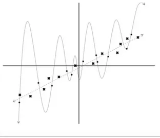
If the case is not a problem solution but a discovery of a correlation or anything interesting, unsupervised learning can be used (Figure 2.1). Machine can make a prediction with unsupervised algorithm on a given data and try to cluster them without any label. Then the user can put the label on the clusters or take them as a precursor to the research of interest.

Figure 2 1 Clustering as an unsupervised learning

By putting these two algorithms together with semi-supervised learning algorithm machine can try to classify huge amount of data with unsupervised learning and when user put some label on the classes, the algorithm assigns these given labels and proceed supervised learning.

(17)

10

2.1.3. Reinforcement Learning

In reinforcement learning machine is considered as an agent that makes decisions like biological organisms (Figure 2.2). Machine classifies all information as the process of penalty-award decision. All the decisions the agent make is evaluated and improved by having experiences on the new problems without explicitly programmed to behave in a specific way.

Figure 2 2 Reinforcement learning teaches the robot what to choose by penalty and award feedbacks. When the robot chooses the fire it gains a penalty and learns next time to avoid from fire.

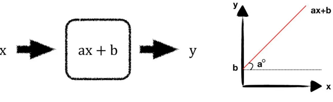
2.2 Supervised Learning

2.2.1. Linear Regression

Linear regression is one of the basic models in the field of statistics. Linear models are fundamentals and studied in the field of mathematics for decades. The simplest linear equation is 𝒂𝒙 + 𝒃 which 𝒂 is the slope of line and 𝒃 is the interception point on the y axis (Figure 2.3). Regression is the calculation of the correlation between the mean value of one variable and corresponding values of another. In this learning algorithm, linear model and regression model are combined to predict the output label y from input features x.

(18)

11

Figure 2 3 Line equation

Here is the mean value of X features of a data with a relation to the Y output values is measured by linear regression model.A linear regression formula is the following:

𝒚 = 𝒘[𝟎]. 𝒙[𝟎] + 𝒘[𝟏]. 𝒙[𝟏] + ⋯ 𝒘[𝒏]. 𝒙[𝒏] + 𝒃

This is the regression version of a data with n features. 𝒘[𝟎] is a weight parameter corresponding to the slope of the equation of 𝒘. 𝒙 + 𝒃 where b is the y intercept corresponding to the bias parameter. For a data set with a single feature gives the line equation of the following:

y= 𝒘. 𝒙 + 𝒃

When the number of feature increases weight of the parameter is taken as matrices in the shape of (𝒏, 𝒎) where n is the number of samples and m is the number of features. Thus, the prediction is done by the weighted sum of all the features with weights and biases.

(19)

12

In the figure above (Figure 2.4) regression model is shown. Here the data is only one dimensional which means one feature corresponds to the output label. As the features increase the dimension of the problem also increases. For example, the prediction of a house price in a city is based on the following features, the place, the size of the house, the type of the house, the amount of room, etc. So, each feature has different amount of contribution to the house price. The regression model tries to predict the price considering all the features. If there is an irrelevant feature in the data it can be excluded.

The application of the linear regression model to the problem can be implemented by the following code (Figure 2.5):

Figure 2 5 Python script for supervised classification problems

In the linear regression model, the distance between prediction and label is measured by cost function. The aim of the learning algorithm is to find a way to minimize the cost. Optimization is a process in which the minimization of these distances provided by adjusting the parameters in training step.

2.2.2. Binary Classification: Logistic Regression

Unlike linear models, logistic regression classifies a problem by giving the probabilistic distribution of output y values. Thus, the prediction is done by decision boundaries which separates the probability of the output labels. Logistic regression makes the prediction by using the following formula:

(20)

13

This formula gives the output either +1 or 0 like a logistic gate. Despite the name of regression this model is a classification algorithm. Like the regression model the formula provides the probability of the points in the feature and label coordinates. Hence, the decision boundary determined by inequality in the formula.

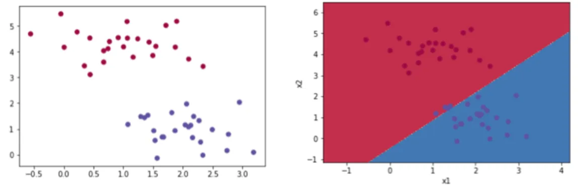
Figure 2 6 An example for logistic regression prepared by blob data set

In this artificial data (Figure 2.6) we want to separate the blobs according to their colors. If we have a binary classification, we can use the model logistic regression. In the figure, the data has two features. For each blob, we know the color and the location on the plane. Our aim is to draw the boundary for the plane so that, different colors are separated from each other. We have the following:

𝐗 = [𝒙_𝟏, 𝒙_𝟐] 𝚯 = [ 𝛉_𝟎, 𝛉_𝟏, 𝛉_𝟐]

Parameter tuning is continuing until finding the best parameter set that gives the accurate results. The parameter search is carried on until the training and testing accuracies are very close to each other. The question is, how do we tune the parameters to make them optimal for the problem? Optimization technique provides us the right parameters by iteratively tuning the model. Thus, the error is minimized and performance is maximized. There are several optimization methods, stochastic gradient descent (SGD), Adams etc. that we’ll be described later on.

In the figure (Figure 2.6), a blob data set is prepared and logistic regression applied with the following code (Figure 2.7):

(21)

14

Figure 2 7 Python script for Logistic Regression

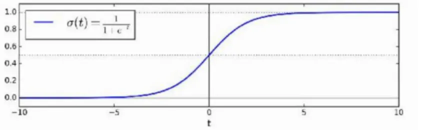
Logistic regression is used for binary classification problem with the sigmoid activation function. It is used for the binary classification problem like whether the picture is cat or dog.

Sigmoid is an activation function is applied to estimate the probability of a label by the threshold of 50%. In logistic regression, the inputs are firstly linearized (like linear regression) then output gives a logistic result with a sigmoid function. The given output is a number between 0 and 1 which represents the choice of category machine does. The sigmoid function and the formula is the following (Figure 2.8):

Figure 2 8 Sigmoid function makes decision in the logistic regression problems either 0 or 1

𝝈(𝒕) = _{𝟏+𝐞𝐱 𝐩(−𝒕)}𝟏 𝒚_{𝒑𝒓𝒆𝒅𝒊𝒄𝒕𝒊𝒐𝒏} = {𝟎, 𝒑 < 𝟎. 𝟓_{𝟏, 𝒑 ≥ 𝟎. 𝟓 (2.1)}

2.2.3. Multiclass Classification: Softmax Regression

Logistic regression can be generalized to multiclass classification by the softmax activation function. Unlike logistic regression, instead of output y, there are categories to which is assigned to a probability between 0 and 1.(Nahid, Mehrabi and Kong, 2018) Softmax activation function distributes the probabilities into output categories by the following formula:

(22)

15

𝑨

_𝒊

=

𝒕𝒊

∑𝒄_𝒊=𝟏𝒕_𝒊

𝒕𝒊= 𝒆𝒛𝒊 𝒛𝒊 = 𝒘𝒊 . 𝑨 + 𝒃 (2.2)

Where A is the feature matrix in the shape of (𝒎, 𝒏) m is the number of samples and n is the number of features, 𝒛_𝒊 is the logits of weighted sum, 𝒕_𝒊 is the exponential of logits, and 𝒄 is the

category number of outputs.

Figure 2 9 A single neuronal unit structure with softmax activation function.

For the multi label classification problems, we use the function softmax, to classify multi label blob data set.

Figure 2 10 As an example, multiclass classification with softmax regression

(23)

16

Figure 2 11 Softmax classification python script

Softmax regression is a generalization model for logistic regression which makes binary classification. With softmax regression multiple choice predictions can be processed, by calculating the probability of scores for each class in a given data set. After linearization function, weighted sums are calculated by the softmax activation function.

The models we used so far was included only one neuronal unit. With one unit and one activation function we can make only linear separations. However, this is not the case in many other problems. As we go further to much more complex problems; such as genome sequencing, pattern recognition our data becomes extremely high dimensional and non-linear.

Deep learning is one of the machine learning algorithm which has a very high capacity to make huge networks.(Learning, 2006) For all of these problems machine learning has an effort to build models with different architectures, by mimicking our brain structure, neural networks, commonly referred as deep learning. The models have been built so far, tackling problems in object recognition and language process has had magnificent success. Recent study shows that a sexual preferences of a person can be recognized by deep neural network. (De Schutter, 2018). Likewise face recognition, these algorithms have potential for future to tackle the problems even humans cannot reach (Buduma and Locascio, 2017).

(24)

17

2.3. Neural Networks

An artificial neuron takes signals as an input, processes it and sends it to the other neuron through axon as an output. Each neural pathway dynamically strengthened or weakened by how often they are used. Biological neurons can be mimicked by creating artificial neuron models to translate the information into computer language.

Figure 2 12 Neuron structure and function description (Buduma and Locascio, 2017)

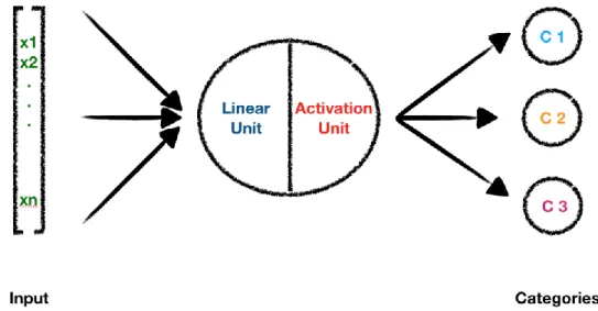
In the Figure 2.13, a functional unit that receives information as features [𝒙_𝟏, 𝒙_𝟐… 𝒙_𝒏] and multiplied by weights [𝒘_𝟏, 𝒘_𝟐… 𝒘_𝒏] are linearized and activated by functions in the neuron units. Linearization function creates logits 𝒁 = ∑ 𝒘_𝒊. 𝒙_𝒊 and activation function can be sigmoid, relu or tanh depends on the problem of choice. The logits are passed through one of these activation function 𝒚 = 𝒇(𝒛) so that, the output can be passed into another unit. The output result can be obtained by carrying out vector multiplications of features and weights with the addition of biases as the following formula;

(25)

18

Figure 2 13 An artificial neuron structure with features vectors X and parameter vectors W

2.3.1. Feed Forward Neural Networks

Technology has enabled us to discover the universe in many aspects. From stars to cells, from galaxies to atoms we’ve built machines that always serve us, make our life easier, make distance closer. Now we are at the edge of machine intelligence. we don’t need to solve the problem by giving instructions to machines, instead we give them what we have; experience, information as data.

Neural networks are mimicking our brain. The way neurons making synapsis and transferring one signal to another is electricity. A baby brain can recognize faces within months and within year babies start to distinguish the voice around them and understand the language.(Kuhn et al., 2006) The way they learn how to separate cat from dog is not by measuring or calculating the features of the objects. First, they are exposed to many images of cats and dogs, then they are reinforced by their parents whether they did something right or wrong. Just like human brain neural networks can distinguish different objects by deep learning which is an active field of artificial intelligence. (Buduma and Locascio, 2017)

(26)

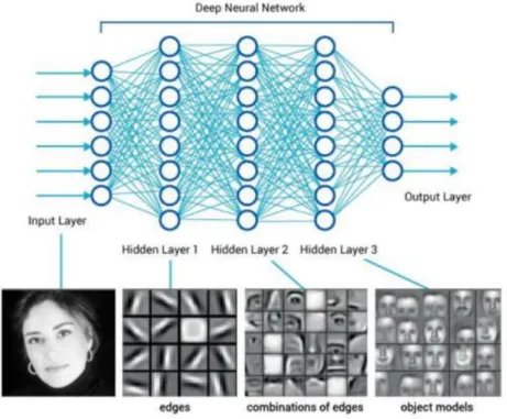
19

Figure 2 14 Deep neural network structure (Deep learning Essentials)

With the method of artificial neural network, input and output data is optimized in a neuron network structure with many layers and units. Each unit acts like a single neuron by taking input data and giving output data. In machine learning, a neuron network is called perceptron Each unit in a perceptron has linearization function and an activation function where aligned by all the layers. In a neural network there are three types of layers; input, output and hidden layers. Input layers are the features of the data and output layers are the labels of the data. On the other hand, in hidden layers all the neurons have activation function either tanh or relu which makes the equation non-linear. For the classification problems, in their last layer all the output neurons have sigmoid function as an activation.

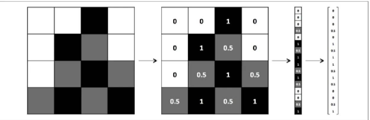
To solve a problem with a machine learning, featurization of a problem should be accomplished. In a problem, featurization is a process to vectorize the features in a way that machine can analyze, efficiently. In the Figure 2.15, there is an example of vectorization of a picture data.

(27)

20

Figure 2 15 Image vectorization process (Buduma and Locascio, 2017)

Our model is defined by the function of 𝒇(𝒙, 𝜽). The input x is the expression of picture in the form of vectors. White, gray and black pixels are given as numbers and translated into vector forms (Figure 2.15). The input 𝜽 is a list of parameters in our model. During learning, our machine tunes the parameter 𝜽 by the help of examples we gave it as an input.

2.3.2. Training Neural Networks

How do we find the best parameters, the weights in between the units, in a neural network? This so-called training process finds the best parameter through a neural network. During training, our data is fed into the neural network and iteratively modify the weights to minimize errors on the model. After training, we’re expecting that our model can solve the problem in the test set with high accuracy.

In the training process, input features are taken and trained by machine learning algorithm by mixing and optimizing weights and biases through hidden layers to make a prediction. This process is called forward propagation. These predictions and ground truth values (labels) are compared with loss functions that tells the distance between the predictions and true labels. After that, penalties are given by cross entropy function as a cost. At the end of the last layer, the predictions are obtained. Second step is backward propagation in which all weights and biases are changed with the derivative of cost functions. This is the way the machine corrects itself. All these steps are count as a single iteration. After many iterations (1000, 10.000 or more) all weights and biases continue to be optimized until the predictions are improved and give higher accuracy.

(28)

21

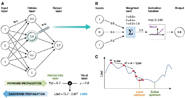
Figure 2 16 Artificial Neural Network training processes (Angermueller et al., 2016)

In the figure (Figure 2.16), a training step is illustrated by forward and backward propagations. (Figure 2.16A) The forward propagation accomplished to the direction from input features to the output layers. At the last layer, output layers yield some predictions to be measured. The measurement gives the difference between the predicted label and the true label as a loss. After many iterations, numerous forward and backward propagations are completed. (Figure 2.16B) When the loss is minimized enough the prediction is reached to the true label. (Figure 2.16C) Shows the minimization process of weight parameters.

2.3.2.1 Loss and Cost Function

In the, neural networks weights and biases are blending to match the input features through the training process. At the end of the layers, all parameters are evaluated by several performance measures. The performance is measured by the calculation of the distance between the prediction vector and the vector of ground truth values (labels). Several measurements are RMSE, MAE and cross entropy. Root mean square error (RMSE) corresponds to the Euclidian distance indicated by L2 norm. The formula is the following,

(29)

22

Where the 𝒉(𝒚) function represents the prediction of the y probability found in this category. And the y is the label. The distance between the label and prediction gives the performance of this model. In other words, it gives how well the model generalizes the data. Mean absolute error (MAE) corresponds to the L1 norm with the following formula:

MAE( X, h(x) ) = _𝒎𝟏∑𝒎_𝒊=𝟏| 𝒉(𝒚) − 𝒚| (2.5)

In each iteration of the training process, the parameters are modified by the aim of minimizing the cost function. Unlike logistic regression in which, the predictions are either True or False, cross entropy gives higher penalty to the wrong answers which is predicted with a higher probability. Calculating loss, with log effect makes it grow very large when the wrong answer is estimated with certainty. In this case, the function doesn’t only evaluate the correctness of the results but also evaluates how much the prediction is close to the correct answer.

The formula of the loss function of cross entropy is the following:

𝓛 = −[𝒉(𝒚) 𝐥𝐨𝐠 𝒚 + (𝟏 − 𝒉(𝒚))𝐥𝐨𝐠 (𝟏 − 𝒚)] (2.6)

At the end of the training, cost function takes the mean of summation for all the loss functions in a single iteration with the following formula:

𝑱 =

𝓛(𝒉(𝒚)𝟏,𝒚𝟏),𝓛(𝒉(𝒚)_𝒎𝟐,𝒚𝟐)…𝓛(𝒉(𝒚)𝒏,𝒚𝒏)

(2.7) 𝑱(𝒘, 𝒃) = _𝒎𝟏∑𝒎 𝓛(𝒉(𝒚)𝒊_{, 𝒚}𝒊₎

𝒊=𝟏 (2.8)

In order for search algorithm to work efficiently and guaranties a solution, cost function 𝑱(𝒘, 𝒃) needs to be convex function of w and b. It gives the penalty for the wrong answers as an adjustment procedure.

2.3.2.2 Gradient Descent

Gradient descent is a general optimization technique which is capable of finding the minimum by tuning parameters iteratively. It gives a convex cost function that only have a global minimum which makes it guarantee to minimize cost function correctly. If we draw a three-dimensional space with two weights w1, w2 on the x and y axis, and error on the z axes we can see the quadratic shape bowl (Figure 2.17).

(30)

23

Figure 2 17 The quadratic error surface for a neuron unit

We can also draw trace of this quadratic bowl with elliptic contours, where the minimum error is at the center. In this set up, elliptic contours are the combination of parameters w1 and w2 for the same Error value. In order to approach the minimum, we need to take perpendicular steps gradually. If parameters of weights and values are chosen randomly, by evaluating the steepest decent and going further through these steps minimum point is reached, shown in the

(Figure 2.18). This algorithm known as gradient descent. It’s a method used in training of

neural networks.

Figure 2 18 Approaching to the global minimum by learning rate (Buduma and Locascio, 2017)

Training a model, actually searching for a parameter set that minimize the cost function over iteration. Hence, it is a search in the parameter space, where each parameter corresponds to a dimension, the more you have it the harder to search for the right combination. Learning rate is one of the hyper parameter to carry out training process. During the optimization process of weights, gradient descent looking for the minimum. Learning rate is our steps to the minimum in gradient descent. If the steps are taken too small, it takes too much time to minimize. However, if it is taken too large it may jump over, means that it may end up a higher position then initial condition (Figure 2.19) (Buduma and Locascio, 2017).

(31)

24

Figure 2 19 If the learning rate taken too large convergence is difficult(Buduma and Locascio, 2017)

2.3.2.3 Preventing Overfitting and Regularization

To select the best model for the data, training parameters should be evaluated on the test set. Possible problems of a model for a specific data set are overfitting and underfitting. In the

(Figure 2.21) there are two models for a bunch of data. If the problem is to predict the y value

with a given x, which model would be best to describe our problem? A twelve-degree polynomial which travels around almost each of the data point or a linear model which is almost getting no training example correct?

Figure 2 20 Splitting data set into train and test sets in order to evaluate training fairly.

In order to decide which model is better, a different set of data should be added to the data set to see how well the models perform (Figure 2.20). Then it is clear that linear model fits data more than 12 polynomial models (Figure 2.22). The key point is that; a model should generalize on the test data without making too much differences with training data. For instance, a very complex model can very strictly fit the data, however on the test data set it may perform very poorly. The situation which the model cannot generalize well enough is defined as overfitting.

(32)

25

This issue becomes more problematic in deep learning where large numbers of neurons and hidden layers take place in the neural network.

Figure 2 21 Linear model and degree 12 polynomial model comparison for training(Buduma and Locascio, 2017)

Figure 2 22 Linear model and degree 12 polynomial model comparison when test data is added (adapted from Buduma and Locascio, 2017)

Overfitting:

If training error is lower than validation error, it means that your model cannot generalize well. The model over fits the data. The polynomial model makes overfitting, because it travels around every each of the data (Figure 2.21).

Underfitting:

The Second model (shown by dashed line) is an example to an underfitting (Figure 2.21). It gives a prediction with high error shows that model cannot generalize the data well enough. It’s like a student only knows the 4 operations of math but try to solve a calculus problem with

(33)

26

derivatives and integrals. The model makes the real problem so simple that any prediction doesn’t approach to the truth values.

Solution to this problem is;

First, model complexity and overfitting should be considered. If the model is not complex enough, training error becomes high because the model cannot train the data enough. On the other hand, if the model is too complex, it is more likely to over fit the data. It’s like a student memorizes every formula in a calculus book but cannot solve any problem other than the book.

Second, to evaluate the model, you need another evaluation set other than training set. Whole data should be split into two set; train and test set. This method provides user to see, how well does the model generalize on unseen data. Third, since the data is trained over iterations, early stopping is used as a regularization to prevent overfitting. To accomplish this, whole training process is divided into epochs. Each epoch is a single iteration with the processes of forward and backward propagation. In order to control your model during training, at the end of each epoch training and validation errors can be controlled. Validation set is also another split from the data. With the validation set, hyper parameters can be searched and tuned. If the training error decreases over iteration while validation error increases, it’s time to stop training because the model has begun to overfitting. Hyper parameter optimization, is the process where the validation set has a very close accuracy to the training accuracy. Best model is selected by looking for the best hyper parameters where the validation accuracy must be confirmed by test accuracy. Comparison between the validation and test accuracy is another confirmation for the user to understand whether hyper parameters have made overfitting.

Regularization:

In order to avoid the problem of overfitting, regularization steps are applied to the model. It prevents the excessive learning during training and reduces the overfitting. If the model under fits the data, training should be increased by splitting more training data or making the model more complex.

There are several ways to prevent training process form overfitting. These methods are; L1 and L2 regularization. Regularization strength is determined by the hyper parameter of lambda during minimization of weights. The larger the lambda, the higher the model is prevented from

(34)

27

overfitting. If L=0 there is no regularization applied to the model. L2 regularization is very common in machine learning. This method provides a homogeny distribution among the input values, instead of using some inputs a lot. In the figure, (Figure 2.23) there is a classification problem in which L2 regularization is applied with L= 0.01, L=0.1, L=1 L2 lambda values.

Figure 2 23 Regularization strengths of 0.01, 0.1 and 1. (Buduma and Locascio, 2017)

The second type of regularization is L1 regularization. It is used for the comprehension of feature distribution, to understand which neuron affects the decision more in a neural network. If the feature analyzes is not important, it is better to use L2 regularization. Moreover, Dropout method prevents the network from being too dependent on any one of the neurons in a layer. By deactivating only some neurons with probability p, neighboring neurons try to handle the representation for the missing neurons. In the (Figure 2.24) you can see how dropout carried out on the neural networks.

Figure 2 24 During training Dropout sets several units inactive in the network with some random probability. (Buduma and

(35)

28

2.3.2.4 Training, Development, Test Sets

In machine learning, 3 different data set is prepared for 3 different generalization error as follows;

Bias, is an error from incorrect predictions in the learning algorithm. High error usually leads to underfitting of the data by missing the relations between features and labels. The Variance, is caused by sensitivity error when the model includes all small variations inside the training set. High variance error occurs usually because, the model learns irrelevant details inside the training set. This situation leads overfitting. Irreducible error, is because of the data itself by nosiness.

A favorable model should be neither biased nor variance. Complex models usually tend to high variance while simple models tend to the high bias. That’s the reason it’s called bias variance tradeoff. Data splitting approaches have developed to avoid bias and variance. In addition to training and testing data sets a validation set should be split from data to make a good parameter estimation.

How do we know that our model is generalizing well on new data set? The only way to understand is to test our model on an unseen data set. If there is more than one model, the best way to understand which model is the best is, to use hold out method. With the holdout method, validation set can be split out from data (Figure 2.25). In general, the ratio of splitting train, validation and test should be 60%, 20%, 20%. The three types of data sets have to be evaluated by their biases and variances which cause the problem of overfitting and underfitting. The solution is; either to train more or prevent more training by regularization.

(36)

29

2.3.3 Recurrent Neural Networks

Language, music and genome have something in common, the structure of sequence. Naturally we are always predicting the future of a sequence when we are listening a speech or a music. In deep learning Recurrent Neural Networks (RNN) can predict the future a little. With RNN, time series data can be analyzed to predict the future price of a product. More generally, RNN can trained on different fractions of sequences rather than fixed sized inputs like Feed Forward Neural Network (FFNN).

Figure 2 26 Recurrent neuron and the unrolled version of it through time

An RNN is very much like a FNNN except they have a feedback loop that pointing themselves in a series of timeline. This structure gives them a second chance to correct themselves during training. In the figure (Figure 2.26) it is shown a single RNN with single input and output on the left side and the unrolled version of RNNs through time on the right side.

The capability of talking to itself of an RNN cell is expressed in the following formula: 𝒚_(𝒕)= 𝝓( 𝒙_(𝒕). 𝒘𝒙+ 𝒚(𝒕−𝟏). 𝒘𝒚+ 𝒃)

(37)

30

Figure 2 27 RNN architectures: sequence to sequence, sequence to vector, vector to sequence and encoder to decoder

(Figure 2.27) RNN architecture can be used in 4 different ways. On the top left graphic

represents the sequence to sequence analyzes. It takes the input as sequence and gives the output also in the form of sequence. On the top right, the structure can be built as sequence to vector. This type of analyzes ignores all the outputs but the last one. On the bottom left, graphic shows from vector to sequence structure. For example, from an input image to an output caption of that image. The last one, on the bottom right shows the encoder-decoder interaction. Encoder takes the input as sequence and gives it to the decoder as vector output, then the decoder takes the input as vector and gives the output in the form of sequence.

RNN can be used for sequence data in many forms however, there are some difficulties for long term training. Training with the RNN algorithm for long sequences brings the necessities of running over many time steps. Generally, this situation brings the problem of vanishing gradients which means that during gradient descent the gradients get smaller and smaller and finally stops converging to the minimum. In addition to long training problem, the memory is another problem for long running RNN. The information in the input neurons are fade away

(38)

31

through time. This may become a series problem, for example in language translations the first word of the sentence may change the meaning with the last word. The algorithm should link the beginning and the final part of the sentence through some memory state. With long term memories, LSTM (Long Short Term Memory) is an alternative for this kind of problems of RNN.

2.3.3.1 Long Short Term Memories

In general, Long Short Term Memories (LSTM) are also neural networks that have basic cells in several layers. Unlike the basic cells, LSTM cells perform much better. Training is converged faster and long term dependencies can be detected with LSTM cells. As the name refers, LSTM has two state vectors: ℎ_(𝑡) h stands for hidden and represents the short term stage. Long term stage is represented by 𝑐(𝑡) and c stands for cell. Briefly, LSTM cells can learn what should be stored in the long term, what should be thrown away and when it should be extracted. (Figure

2.28)

(39)

32

3. Preparation of Data

Learning is a process of generalization of the data into new problems. The data can be used for specific problems or it can be used for open-ended problem like unsupervised learning.

Having clean and appropriate data is the first important thing for a successful machine learning process. A data is composed of rows and columns in which features and samples are filled. In the data processing, features that are in consideration are called attributes and the samples are called instances. For a balance and accurate training results the data should be shuffled and all the attributes should be fulfilled before running the learning process.

Feature selection is a significant process to approach a problem with machine learning. In biological, medical and pharmaceutical fields, the most important thing is the representation of the natural phenomenon as vectors and matrices. This process is called featurization. In bioinformatics problem DNA and proteins can be transformed into vectors. In pharmaceutical problems such as, toxicity measurement, biological activity measurement or protein tertiary structure analysis the chemicals can be transformed into vectors by several approaches, such as physicochemical properties, presence or absence of a specific compounds or geometric characteristics.(Wu et al., 2017)

3.1. Cleaning Data

In a machine learning project, the most time spending part is the cleaning data. Most algorithms cannot work properly with missing data. There are two strategies for a missing data. Either excluding the entire instance or attribute or filling the missing value with zero, mean or median.

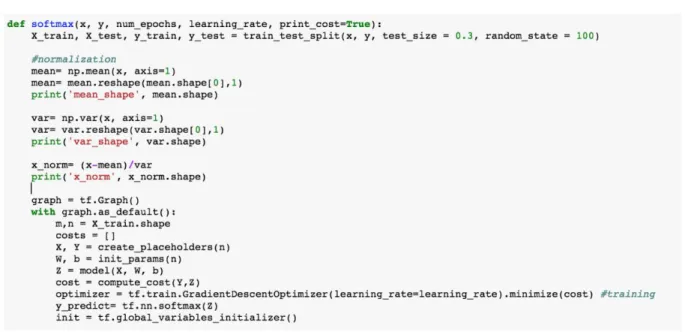
3.2. Input Normalization

In data preprocessing steps, input normalization (min-max scaling) is performed to standardize the data. To make all attributes in the same scale, minimum and maximum values should be scaled. Normalization makes the minimization procedure go faster. The center of the data is calculated by the mean and each value is subtracted by this mean. It makes the data shift back

(40)

33

to the origin. Then the result divided by the variance which calculates how far the data is spread apart. Input normalization is calculated by the following formulas;

Mean= 𝝁 = ∑ 𝒙𝟏 𝒊 𝒎 𝒎 𝒊=𝟏 Variance= 𝝈𝟐 = ∑ (𝒙𝟏 𝒊_−𝝁 𝟏)𝟐 𝒎 𝒎 𝒊=𝟏 (3.1) Normalization= 𝒙_{𝒏𝒐𝒓𝒎}𝒊 = 𝒙 𝒊_−𝝁 𝝈𝟐

The calculation can be implemented by this python script,

Figure 2 28 Input normalization python script

4. Implementing Machine Learning

4.1. Python and Jupyter Notebook

Python has become very popular programming language in recent years. It is used in a very broad field of application with explicit libraries for visualization, statistics, natural language processing, image processing and more. With python the user can directly interact with the code using terminal or different environments like Jupyter Notebook. The main libraries for machine learning are, numpy; which provides the array construction, pandas; data frame construction and manipulation, scikitlearn; machine learning functions, matplotlib; visualization for plots, histograms and creating artificial data.

(41)

34

4.2. Tensor Flow

Tensor Flow is a python library that we can perform highly complicated computations with a graph by flowing through the data as tensors (Figure 2.29). In this graph two edges (data) connected each other by nodes (mathematical operations). Data can be 1D tensor like vectors, 2D tensor like matrices in Tensor Flow. In order to build a deep learning network model with Tensor Flow, variables are used to represent the parameters. Unlike other tensors, variables are kept in the computational graph model. By each iteration, variables can be modified by gradient descent and can be saved for later use. Tensor Flow apply transformations to the tensors in the computational graph such as, elementwise mathematical operations, array operations, matrix operations etc. To pass the input data into our deep model we use placeholders. It is efficient because it is not initialized once like variables do. Instead, it is fed by data in every run in the computational graph. With variables, placeholders and operations we can draw a computational graph. With Tensor Flow sessions we can initiate and run the whole graph.

(42)

35

4.3. Keras

Keras is a python deep learning library. It is a high level neural network API (Application Programing Interphase), written in python. Tensor Flow, CNTK and Theano are the backend for Keras. Thus, it is capable of very fast experimentation with CPU and GPU. It is very user friendly, powerful and fast. With the Keras library, a simple neural network can be built in just a few lines. Modifying and evaluating the result with the Keras is very quick and efficient.

There are two types of usage for Keras; Sequential Modelling and Functional API. Sequential Modelling has neural network architectures, several optimization options, accuracy metrics and fitting methods. This gives the user a flexible and creative way of writing machine learning algorithms. The second option is Functional API. It gives more freedom, more words and more work to the user. With Tensor Flow backend, Keras has a higher capacity for expression of the computational demands.

5. Data sets

5.1 Anuran Call

Anurans (frog or toads) are important for the ecosystem and they are used as earl indicators for ecological stress. Their calls are indicator of their behavioral and biological differences. Thus biologist analyze anuran calls by processing the voice frequency which has enough information to identify an anuran species. (Colonna et al., 2016)

Mel- Frequency Cepstral Coefficient (MFCCs) are one of the most popular technique to present the audio signal as features in speech recognition. Therefore, data set is prepared for the challenge of detection of the species of anuran from its voice. This data set is created from 60 audio record of individual frog which belongs to 15 species. (Figure 5.1) For the segmentation process of audio frames into syllables, spectral entropy and binary cluster method is used. At the end of segmentation 7195 syllables are obtained. from each syllable 22 MFCCs are extracted and normalized between -1< mfcc <1 (Colonna et al., 2016).

(43)

36

For the machine learning process 7195 syllables are considering as instances and 22 MFCCs are the attributes. At the last column, frog species labels are located.

All family labels are;

Anuran Species The amount of species in the Data set AdenomeraAndre AdenomeraHylaedact… Ameeregatrivittata HylaMinuta HypsiboasCinerascens HypsiboasCordobae LeptodactylusFuscus OsteocephalusOopha Rhinellagranulosa ScinaxRuber 672 3478 542 310 472 1121 270 114 68 148

Figure 5.1 Processing anuran calls for classification. (Colonna et al., 2016)

5.2 Thyroid Patients

This data set is a combination of different medical sources about thyroid. The goal is to detect whether the patient is healthy, hyperthyroid or hypothyroid. There are 72,000 patients’ records with 21 attributes, which is shown in the table:

(44)

37

Table 6 1 Thyroid patients attributes

5.3 E. coli

This data set predicts the localization site of a protein in the prokaryotic organism E. coli. There are 336 instance and 8 attributes for the E. coli data set.

Attributes

mcg: McGeoch's method for signal sequence recognition. gvh: von Heijne's method for signal sequence recognition. lip: von Heijne's Signal Peptidase II consensus sequence score. chg: Presence of charge on N-terminus of predicted lipoproteins.

aac: score of discriminant analysis of the amino acid content of outer membrane and periplasmic proteins. alm1: score of the ALOM membrane spanning region prediction program.

(45)

38 Class Labels

cp (cytoplasm)

im (inner membrane without signal sequence) pp (perisplasm)

imU (inner membrane, uncleavable signal sequence) om (outer membrane)

omL (outer membrane lipoprotein) imL (inner membrane lipoprotein)

imS (inner membrane, cleavable signal sequence)

5.4 HIV

In the Human Immunodeficiency Virus (HIV) data set 746, 1625, schilling and Impens data sets are concatenated to 6,590 instances. The attributes are 8 letter strings as octamers and a binary label that tells whether this octamer is cleaved by the HIV cleavage enzyme. Octamer strings are 8 letter amino acids which vectorized into numbers. Each number corresponds to one of the 20 amino acid. This problem is a binary classification. The aim of machine learning in this data set is to analyze the octamer sequence whether they are cleaved by enzyme or not.

6. Results and Discussions

All data sets are applied to different machine and deep learning algorithms gradually. From single neuronal unit to multi layers and from multi-layer to recurrent cell. Single cell can classify the problem by linear division. However, neural networks have additional neuronal units with non-linear activation function. This non-linearity gives model to draw a flexible division.

(46)

39

6.1 Softmax Classifications

The simplest approach to apply is a single neuronal unit. Each data sets are classified linear separation with sigmoid and softmax function. For binary classification problems like HIV data sigmoid is used because it gives an output either 0 or 1. Frog, thyroid and E. coli data sets are multi label classifications. Therefore, softmax classification gives a probability distribution between 0 and 1. Table 6.2 shows training and testing accuracies of the four data sets. In order to increase an accuracy there are 3 ways to apply. First, finding a better optimizer which we already changed the optimizer to ADAM. Second, train more which we already train long enough so that, the line is flattened enough. Final approach is, using a complex model. Thyroid data set shows a very high accuracy. However, Frog, HIV and E. coli data need to be improved with a complex model strategy. E. coli data set cannot be implemented to a more complex model because it has only 336 instances and model with this much parameter would be very flexible. And flexible models are over fits the data. In other words, they have high variance error. Finally, all the results are calculated according to the accuracy metric. The formula is the following:

𝐴𝑐𝑐𝑢𝑟𝑎𝑐𝑦 =_{𝑡𝑝+𝑡𝑛+𝑓𝑝+𝑓𝑛}𝑡𝑝+𝑡𝑛 (6.1)

In the (Table 6.2), the accuracy and loss plot results are shown for all different data sets. For HIV data 5.000 iteration is applied with 10−3_{learning rate. The training and testing accuracy} are 81% and they are the same. The closer the training error and testing error the higher consistent of the learning. However, 81% accuracy can be improved by a higher complex model like Feed Forward Neural Network. For the thyroid patient data set, 5,000 iteration is applied with 10−3_{learning rate. The accuracy is very high and the plot lines are the same which means} a successful prediction. For the E. coli data set, 20,000 iterations are applied with 10−3_learning. The training and testing error are the same. Finally, in the frog data set, 5,000 epochs (iterations) are done by 10−3 learning rate and the accuracy is 78% with both training and testing. Like HIV data, frog data set can be improved with a higher complex model.

For softmax multiclass classification algorithm all learning process is optimized by ADAM optimizer. It is a strengthen form of gradient descent. It makes the minimization quicker and more sustainable. The other optimizers, SGD (Stochastic Gradient Descent), RMSprop (Root Mean Square Propagation) are also tested. It can be concluded that, from all the different optimizers ADAM is the most effective one for our data sets.

(47)

40

Table 6 2 Loss and training accuracy plots of softmax multiclass classification

In the (Table 6.3) the training and testing accuracies are compared with all different data sets. It is concluded that; Frog and HIV data set can be implemented to a neural network which has more complex structure with multiple layers and units.

(48)

41

Table 6 3 Softmax Classification on 4 different Data sets

6.2 Classification using Feed Forward Neural Networks

Frog and HIV data set can be improved by Feedforward Neural Network (FFNN). Unlike softmax classification, FFNN can have more complex architecture so that, it can give more accurate results. Constructing a neural network is a state of art approach. How many hidden layers should be added? How many neuron units should be included? Do they have to be symmetric or not? All these situations are depending on the problem, data and computer power, time etc. There is no strict rule to build a neural network architecture. However, there are several rule of thumbs method (Heaton, 2008) ;

• The number neurons should be between the size of the input layer and the output layer. • The number neurons should be 2/3 of the attributes plus the labels.

• The number neurons should be less than twice the size of attributes.

These methods can be considered as a beginning of trial and error process of model selection. Building a neural network, splitting and shuffling the data are the first step of FFNN. Running and parameter tuning is the second step. The first and second part of FFNN should be considered as separate. If different models are examined on different split of data, the

(49)

42

predictions cannot be fair. Therefore, after the model selection trials can be proceed by regularization steps in which hyper parameters are evaluated.

Frog data is applied to several different Neural Network models. (Table 6.4) shows the selected models. Model 1 has two hidden layers with 7 neuron units and Model 2 has 22 neuron units with 2 hidden layers. It is selected to make a comparison with accuracy levels between a very complex and rather simple structure. Learning rate is chosen as 10−3 with ADAM optimizer. Different activation functions such as tanh, relu are both applied and tanh activation function shows a better performance. Each neuron unit has one linearization unit and one activation part. The selection of tanh and relu are for the hidden layer neurons. On the other hand, softmax is also an activation function but it is applied only on the output layer neuron units. More specifically, softmax functions are capable of multilayer classifications. In this example frog data set are meant to predict the species of a frog from the audio record. And there are 15 different frog species which gives 15 neuronal units with softmax activation function in the output layer.

Table 6 4 Different 2 FFNN models for frog data set

(Table 6.5) shows the loss and accuracy plot for Model 1 and Model 2. The difference between

the training and validation shows how well the machine learns the parameters. In the Model 1 the difference is around 0.3% and in the model 2 it is almost 2.0% which tells that Model 1 is better than Model 2. Also it can be seen that, on the second model training and validation lines (the blue and orange lines) are breaks apart at the end of the iterations. However, in the first model it was overlapped. Furthermore, these results are not strict and can be varied with the epoch numbers. Here we choose to run the plot with 200 epochs. As it is seen, the loss plot approach to zero and becomes steady.

(50)

43

Table 6 5 Loss and Accuracy plot for Model 1 and Model 2 Multilayer Perceptron

Model 1 with 96% accuracy can be regularized and the difference between the training and validation can be decreased. L2 and Dropout methods applied with 3 different regularization steps (Table 6.6).

(51)

44

Table 6 6 Regularizations for Frog FFNN Model 1

In the (Table 6.7) Frog species Model 1 with 3 different regularizations are shown with their loss and accuracy plots. For each plot 200 epochs are applied. Regularization 2 with 0.1 dropout is the best form of Model 1 because training and validation accuracies are almost the same. However, in regularization 3, both dropout and L2 is too much and the distance has increased a little bit.

(52)

45

(Table 6.8) shows the train and validation accuracy for the frog species Model 1. The next step

is to test the best model and best regularization with a test set as a third split. The validation set indicates the overfitting in the training set by analyzing the parameters. The test is like a double check for consistent learning by analyzing the hyper parameters. Therefore, the best accuracy is calculated after prediction on the test set.

Table 6 8 Evaluation for the best regularization decision for the frog species Model 1

Table 6 9 Implementation of test set and prediction accuracy for frog species data set.

Finally, (Table 6.9). Shows the improvement of the accuracy for Frog Species data set. Softmax multiclass classification gives the 78% accuracy and Feed Forward Neural Network has developed this result to 95% accuracy.

(53)

46

HIV Data set

With the Softmax multiclass classification algorithm, HIV cleavage sites are predicted up to 81% accuracy. Softmax is a single neuronal unit and we can develop Model 1 and Model 2

(Table 6.10). Both of two models have ADAM optimizer and relu function for the activation

unit and they minimized gradient descent with 10−3_{learning rate. Model 1 has 2 hidden layers} with 7 neuronal units which makes it simpler than Model 2. This number has chosen by the rule of thumb strategies, mentioned earlier. Model 2 has 13 units in each layer which also gives reasonable parameters with respect to attributes given to the model. Moreover, if the performance doesn’t differ much when two models are compared, the simpler model is preferred to the complex one.

Table 6 11 HIV Model 1 and Model 2 with Feed Forward Neural Network

In the table above (Table 6.11) Model 1 and Model 2 is chosen to show how well the accuracy on rather simple and complex models. Learning rates, optimizers and activation functions are chosen as it is shown on the table.

(54)

47

(55)

48

Table 6 13 Model comparison for HIV cleavage site data set.

(Table 6.13) shows the different regularizations applied for Model 2. Dropout and L2 is put on

the model gradually. The one with two regularizations causes overfitting.

Table 6 14 The test accuracy result for the best regularization of HIV Model 2

Finally, the test split also implemented to the model in order to see the final accuracy of Model 2 for HIV data set (Table 6.14)

(56)

49

6.3 Long Short Term Sequence Memory (LSTM)

When the test results are compared with Softmax and FFNN on (Table 6.14) and (Table 6.3), HIV data set has not improved a lot. It is because the data is composed of short octamer sequences. This data set is a binary classification problem which can be implemented by sigmoid function on logistic regression or softmax activation function on softmax classification. However, the problem is not the labels but the attributes. It is a sequence data which means before and after of an amino acid should be considered as a pattern. Since the data is sequential, we also tried a sequential model: the Long Short Term Memory (LSTM) model. (Table 6.15) shows the LSTM implementation for HIV data set with; total number of amino acids, max review length and embedding vectors as a single octamer length. Memory Cell is the hyper parameter for memory. In this case it keeps the value of weights and biases in the memory and connects them with an ulterior attribute.

Table 6 15 LSTM model structure for HIV data set.

LSTM architecture has an additional layer in the neural network. (Table 6.15) shows the hyper parameters of LSTM layer. The total amino acids number is 52.720 and all individual sequences are octamer (8 amino acids). If they were in different lengths max review length hyper parameter can truncate and pad the sequences so that they can be in the same length. Embedding vector keeps the location information of an amino acid in a sequence. Moreover, with memory cells (smart neurons) LSTM network keep the information during training for long sequences. We used sigmoid activation function because the problem is binary classification.

(57)

50

Table 6 16 LSTM regularizations

Here in (Table 6.16) different regularizations are applied gradually and the best hyper parameters are searched.

(58)

51

(Table 6.17) shows different regularizations applied to LSTM neural network. Regularization

1 and 3 have shown a very similar effects on LSTM. Over 500 iterations regularization 1 and 3 shows a very clear accuracy plots (Table 6.18). Regularization 1 is very tending to overfitting however, regularization 3 shows a perfect overlapping.

Table 6 18 Comparison plots for LSTM regularization with longer training

(59)

52

(Table 6.19) Shows the testing accuracy for regularization 3 in comparison to the LSTM with

no regularization.

Table 6 20 The final comparison for HIV sequence data for Softmax, FFNN and LSTM algorithms.

Finally, HIV cleavage site sequence data has implemented on Softmax, FFNN and LSTM algorithms and as it is seen on the (Table 6.20) it is improved from 81% to 92% accuracy with LSTM.

(60)

53

7. Conclusion

In conclusion, machine learning and more specifically deep learning algorithms are applied on 4 different data sets: Frog species identification, Thyroid diagnoses, determination of E. coli protein localization and activation analyzes of HIV cleavage cite sequence. All types of problems are analyzed by, first a single neuronal unit Softmax and then Feed Forward Neural Network. The improvement is analyzed in terms of training and testing errors. On the other hand, HIV sequence data is classified using an LSTM model, which is a special kind of RNN model. With this master study, it is shown that, deep learning is an effective and promising tool for understanding complex biological systems in a variety of fields by discovering: patterns, correlations between the diagnosis and diseases and drug targets.