BROADBAND DOUBLE-MATCHING VIA LOSSLESS
UNSYMMETRICAL LATTICE NETWORKS
Metin ŞENGÜL
Kadir Has University, Dept. of Electronics Engineering,
Faculty of Engineering and Natural Sciences, 34083, Cibali-Fatih, Istanbul, Turkey Tel: +90-212-533-6532, Fax: +90-212-533-4327
Abstract: In this paper, a broadband double-matching network design algorithm has been presented. In the network, an unsymmetrical lattice network has been used. The branch impedances of the lattice network are composed of singly terminated lossless LC networks. After giving the procedure, its usage has been illustrated via an example.
Keywords: Broadband networks; Lossless networks; Lattice networks; Broadband matching; Synthesis.
1. Introduction
Broadband matching network design is an essential problem for microwave engineers [1]. So analytic theory of broadband matching [2-3] and computer-aided-design (CAD) methods are two essential tools for them [4-6]. But it is well known that analytic theory is difficult to utilize even if the source and load impedances are simple. Therefore, it is always preferable to use CAD methods. All the CAD techniques optimize the matched system. But this optimization is highly nonlinear and requires very good initial values [7]. As a result, initial element values are extremely important for successful optimization.
The matching problem can be classified basically as filter, single matching, double-matching and active two-port problems. If both terminating impedances are resistive, it is a filter problem. In single matching problem, generator impedance is resistive and load impedance is complex. If both terminating impedances are complex, then the problem is referred to as the double-matching problem. If the input and output of an active device is simultaneously matched to given load and generator impedances, then this is called as the active two-port problem. Design of a microwave amplifier is a typical example of this matching problem.
In matching network design problems, ladder networks are preferred, since these structures
have very low sensitivity [8]. If one requires more than one path of transmission between the input and output ports, this can be realized by parallel or bridged structures. Without the common ground between the input and output ports, right half-plane zeros can be realized by a bridge structure. If the bridge leads are twisted, the configuration seen in Fig. 1 is obtained, which is known as an unsymmetrical lattice network [9].
Figure 1.Unsymmetrical lattice network with complex
terminations.
Therefore, in this paper, two-port bridge structures are utilized in broadband double-matching networks. The proposed method generates very good initials to improve the matched system performance by optimizing the element values via commercially available CAD tools. In the following section, real frequency broadband matching will be summarized. Then, the design algorithm and an example will be presented.
2. Real frequency broadband matching
The matching conditions of the complex load ZL to the complex generator ZS can be formulated in terms of the normalized reflection coefficients at ports 1 and 2. The input reflection coefficients 1 can be defined byS in S in Z Z Z Z * 1 (1)
where Zin is the input impedance seen at port 1 when port 2 is terminated by the load ZL. Similarly the reflection coefficient at port 2 can be defined by
L out L out Z Z Z Z * 2 (2)
where Zout is the impedance seen at port 2 when port 1 is terminated by the source impedance ZS, and the upper asterisk denotes complex conjugation. Here, 2 is the normalized reflection coefficient at port 2. Since the two-port is considered as lossless, we have on the imaginary axis of the complex frequency plane
2 2 2
1
(3)
Then, the transducer power gain (TPG) at real frequencies can be expressed as
2 2 2 1 1 1 ) ( TPG (4)
The goal in broadband matching is to design the lossless network N, which consists of the arm impedances Z1(p),Z2(p),Z3(p) and
) ( 4 p
Z , such that TPG() given by Eq. (4) is maximized inside a desired frequency band. Obviously, maximizing TPG() means to minimizing the modulus of the reflection coefficients 1 or 2 . In this context, the matching problem is reduced to the determination of a realizable impedance function Zin or Zout.
Let the equalizer input impedance Zin be expressed in terms of its real and imaginary parts on the real frequency axis as
) ( ) ( ) ( in in in j R jX Z (5)
By using Eq. (5), Eq. (4) and Eq. (1) we obtain transducer power gain in terms of the real and imaginary parts of the input impedance Zin
and the source impedance
) ( ) ( ) ( S S S j R jX Z as follows: 2 2 )) ( ) ( ( )) ( ) ( ( ) ( ) ( 4 ) ( in S in S in S X X R R R R TPG (6)
Namely the matching problem consists of finding Zin(j) such that TPG() is maximized inside a desired frequency band. Once Zin is
determined properly, the equalizer network N can be synthesized directly by using the obtained impedance or the corresponding reflection coefficient.
3. Rationale of the matching procedure
For a lossless two-port like the one shown in Fig. 1, the canonic form of the scattering matrix is given by [10,11] ) ( ) ( ) ( ) ( ) ( 1 ) ( ) ( ) ( ) ( ) ( 22 21 12 11 p h p f p f p h p g p S p S p S p S p S (7) where pj is the complex frequency variable, and 1 is a unimodular constant. If the two-port is reciprocal, then the polynomial f( p) is either even or odd. In this case, 1 if f( p) is even, and 1 if f( p) is odd.For a lossless 2-port, energy conversation requires that I p S p S( ) T( ) , (8)
where I is the identity matrix. The explicit form of Eq. (8) is known as the Feldtkeller equation and given as
) ( ) ( ) ( ) ( ) ( ) (p g p h p h p f p f p g . (9)
In Eqs. (7) and (9), g( p) is a strictly Hurwitz polynomial of nth degree with real coefficients, and
) ( p
h is a polynomial of nth degree with real coefficients. The polynomial function f( p) includes all transmission zeros of the two-port.
Consider the bridge network seen in Fig. 1 or Fig. 2. Since it is not desired to dissipate any power in the impedances Z1(p),Z2(p),Z3(p) and Z4(p), they
must be lossless, so they must be composed of only inductors and capacitors. Also their terminations must be either short or open, not resistive terminations. So these impedances are singly terminated lossless LC networks [12].
In [12], it has been shown that for a lossless singly terminated network, the input reflection coefficient can be expressed as
) ( ) ( ) ( ) ( ) ( 11 p g p g p g p g p S (10)
where 1 and 1 corresponds to an open and short termination, respectively. So the procedure proposed in [12] can be used to design the impedances
) ( ), ( ), ( 2 3 1 p Z p Z p
Z and Z4(p). Then the following algorithm is used to design the broadband matching network by using unsymmetrical lattice networks.
Algorithm
Inputs
i(actual)2fi(actual); i1,2,,N: Measurement or calculation frequencies selected arbitrarily.
N: Total number of measurement or calculation frequencies.
ZL(actual)(ji)RL(actual)(i) jXL(actual)(i) ; i1,2,,N: Measured or calculated load impedance data at N frequency points.
ZS(actual)(ji)RS(actual)(i)jXS(actual)(i) : i1,2,,N: Measured or calculated source impedance data at N frequency points.
fNorm: Normalization frequency.
R0: Normalization resistance, usually 50. nk; k1,2,3,4: Desired number of elements in the arms of the bridge network.
k 1; k1,2,3,4: Desired termination type of the arms of the bridge network.
gk( p); k1,2,3,4: Initialized polynomial )
( p
g describing the arm impedances of the bridge network.
T0: Desired flat transducer power gain level.
: The stopping criteria. For many practical problems, it is sufficient to choose 103. Computational Steps
Step 1: If the given load and source impedances and frequencies are actual values, not normalized, then normalize the frequencies with respect to
Norm
f and set all the normalized angular frequencies Norm actual i i f( )/ f .
Normalize the load and source impedances with respect to normalization resistance R0 over the entire frequency band as
0 ) ( 0 ) ( /R ,X X /R R RL Lactual L Lactual , 0 ) ( 0 ) ( /R ,X X /R R RS Sactual S Sactual .
It should be noted that if the load and source is specified as admittance data, then the normalization resistance R0 multiplies the real and imaginary parts of the admittance data (i.e.,
0 ) ( 0 ) ( R ,B B R G GL Lactual L Lactual , 0 ) ( 0 ) ( R ,B B R G GS Sactual S Sactual ).
But if the given load and source impedances and frequencies are already normalized, and then go to the next step directly without any normalization process.
Step 2: Calculate the input impedance values of the arms of the bridge network as
N i and k j S j S j Z i k i k i k , , 2 , 1 4 , 3 , 2 , 1 , ) ( 1 ) ( 1 ) ( 11 ), ( 11 ), ( ) ( (11) where ) ( ) ( ) ( 11 ), ( i k i k k i k j g j g j S is the input
reflection coefficient of the arms of the bridge network. Step 3: Calculate the input impedance of the bridge network when port 2 is terminated by the load impedance ZL via the following equation,
D N Zin (see Fig. 1), where
4 3 2 3 2 4 2 4 2 4 3 3 2 3 4 1( ) Z Z Z Z Z Z Z Z Z Z Z Z Z Z Z Z Z Z Z Z N L L L L and L L L L Z Z Z Z Z Z Z Z Z Z Z Z Z Z D 3 4 3 4 2 3 2 4 2 1( )
The input impedance expression has been obtained by using toY transformation equations [13].
Step 4: Calculate transducer power gain via Eq. (6) as follows 2 2 ( ( ) ( )) )) ( ) ( ( ) ( ) ( 4 ) ( i in i S i in i S i in i S i X X R R R R TPG where RS(i)Real(ZS(ji)), Rin(i)Real(Zin(ji)), )) ( ( Im ) ( i S i S aginaryZ j X ,Xin(i)Imaginary(Zin(ji))
Step 5: Calculate the sum of the squared error via
N i i C j 1 2 ) ( where (ji)T0TPG(i). Step 6: If C , synthesize ) ( ) ( ) ( 11 ), ( p g p g p S k k k k and obtain the arm networks of the bridge, then stop. Otherwise, change k (termination types) and/or
) ( p
gk (initialized polynomials) via any optimization routine and go to Step 2.
The algorithm explained above has been applied to broadband single-matching problems in [14]. But in this paper, the method is utilized to broadband double-matching problems.
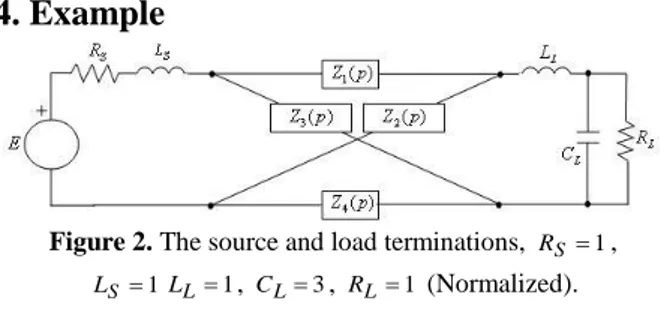
4. Example
Figure 2. The source and load terminations, RS 1, 1
S
L LL1, CL3, RL1 (Normalized). In this section, an example will be given to illustrate the proposed algorithm. Here all the calculations will be made by using normalized values. After designing the matching network, all components
can be de-normalized by using the given normalization frequency (fNorm) and resistance (R0).
The source and load impedances in normalized values can be seen in Fig. 2. So there is no need a normalization process. In Table 1, the calculated source and load impedance values are given.
Table 1. Given normalized source and load impedance
data RS XS RL XL 0.1 1.0 0.1 0.9174 -0.1752 0.2 1.0 0.2 0.7353 -0.2412 0.3 1.0 0.3 0.5525 -0.1972 0.4 1.0 0.4 0.4098 -0.0918 0.5 1.0 0.5 0.3077 0.0385 0.6 1.0 0.6 0.2358 0.1755 0.7 1.0 0.7 0.1848 0.3118 0.8 1.0 0.8 0.1474 0.4450 0.9 1.0 0.9 0.1206 0.5743 1.0 1.0 1.0 0.1000 0.7000
The selected initial coefficients of the polynomials (gk(p)), the alpha constants (k) and the desired flat transducer power gain level (T0) are as follows, g1
6 20 3
,
6 7 1
2 g , g3
13 6 1
, g4
1 13 12
, 1 1 , 2 1, 31, 41, and 8 . 0 0 T , respectively.After running the proposed algorithm, the following polynomial coefficients and alpha
constants are obtained,
0.001 21.6652 1.9256
1 g ,
8.3578 4.1205 0.001
2 g ,
14.1635 4.1955 0.3547
3 g ,
0.001 17.8068 10.4634
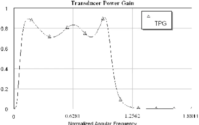
4 g , 11, 1 2 , 3 1, 4 1, respectively.After synthesizing the corresponding reflection coefficients the bridge network seen in Fig. 3 is reached. The obtained transducer power gain curve is given in Fig. 4.
Figure 3. Designed matching network, L14.6157105, 2511 . 11 1 C , L24120.5, C22.0284, L311.8283, 3759 . 3 3 C , L41.7019, C45.6158105 (Normalized).
Actual element values can be obtained by de-normalization. So actual element values are given by
. ) Re ( Re , ) 2 / ( , / ) 2 / ( 0 0 0 R sistor Normalized sistor Actual R f Inductor Normalized Inductor Actual R f Capacitor Normalized Capacitor Actual Norm Norm
Since the matching network is designed by using normalized values, the cutoff frequency of the network is 1 (see Fig. 4). After de-normalization process, it shifts to the given normalization frequency, since fi(actual)ifNorm.
As can be seen in Fig. 4, a fluctuating transducer power gain curve is obtained within the required frequency band at the desired flat gain level (T0 0.8).
5. Conclusions
An algorithm has been proposed to design broadband impedance matching networks via lossless unsymmetrical lattice networks. Since it is not desired to dissipate power in the equalizer, the arm impedances of the lattice network are selected as singly terminated lossless LC sections. In the paper, double-matching problem (complex source and complex load impedance) has been considered.
In the example, the desired flat transducer power gain level is selected as 0.8. As can be seen from the transducer power gain graph, a fluctuating gain curve around this level has been obtained.
It is shown that the proposed method generates very good initials to improve the matched system performance by optimizing the element values. Therefore, it is expected that the proposed algorithm can be used as a front-end for the commercially available CAD tools to design broadband matching networks for communication systems.
Figure 4.Transducer power gain curve.
6. References
[1] B. S. Yarman, “Broadband Networks”, Wiley Encyclopedia of Electrical and Electronics Engineering, 1999.
[2] D. C. Youla, “A new theory of broadband matching”, IEEE Trans. Circuit Theory, vol.11, pp.30-50, 1964.
[3] R. M. Fano, “Theoretical limitations on the broadband matching of arbitrary impedances”, J. Franklin Inst., vol. 249, pp.57-83, 1950.
[4] Awr: Microwave office of applied wave research inc. www.appwave.com.
[5] Edl/ansoft designer of ansoft corp. www.ansoft.com/products.cfm.
[6] Ads of agilent techologies. www.home.agilent.com. [7] B. S. Yarman, M. Şengül, A. Kılınç, “Design of
practical matching networks with lumped-elements via modeling” IEEE Trans. on Circuits and Systems I: Regular Papers, vol.54(8), pp.1829-37, 2007. [8] W. K. Chen, “Passive and active filters”, Wiley,
New York, 1986.
[9] W. C. Yengst, “Procedures of Modern Network Synthesis”, The Macmillan Company, New York, 1964.
[10] V. Belevitch, “Classical Network Theory”, Holden Day, San Francisco, 1968.
[11] A. Aksen, “Design of lossless two-port with mixed, lumped and distributed elements for broadband matching”, Dissertation, Bochum, Germany: Ruhr University, 1994.
[12] M. Şengül, Reflectance-based foster impedance data modeling, Frequenz Journal of RF Engineering and Telecommunications, vol.61(7-8), pp.194-6, 2007. [13] J. W. Nilsson, “Electric Circuits”, Addison-Wesley,
New York, 1993.
[14] M. Şengül, “Broadband impedance matching via lossless unsymmetrical lattice networks”, Int. J. Electron. Commun. (AEU), vol: 66(1), pp: 76-79, Jan. 2012.
Metin ŞENGÜL received his
B.Sc. and M.Sc. degrees in Electronics Engineering from Istanbul University, Turkey in 1996 and 1999, respectively. He completed his Ph.D. in 2006 at Işık University in Istanbul, Turkey. He worked as a technician at Istanbul University from 1990 to 1997 and was a circuit design engineer at the R&D Labs of the Prime Ministry Office of Turkey between 1997 and 2000. He was employed as a lecturer and assistant professor at Kadir Has University, Istanbul, Turkey between 2000 and 2010. Dr. Şengül was a visiting researcher at the Institute for Information Technology, Technische Universität
Ilmenau, Ilmenau, Germany in 2006 for six months.
Currently, he is an associate professor at Kadir Has University, Istanbul, Turkey and working on microwave matching networks/amplifiers, device modeling, circuit design via modeling and network synthesis.