Received 16 November 2013, Revised 23 November 2015, Accepted 26 November 2015 Published online 13 January 2016 in Wiley Online Library (wileyonlinelibrary.com) DOI: 10.1002/asmb.2154
On the Modeling of CO
2
EUA and CER Prices of
EU-ETS for the 2008–2012 Period
¨
Ulkü Gürler
a*†, Deniz Yenigün
b, Mine Ça˘glar
cand Emre Berk
dIncreased consumption of fossil fuels in industrial production has led to a significant elevation in the emission of greenhouse gases and to global warming. The most effective international action against global warming is the Kyoto Protocol, which aims to reduce carbon emissions to desired levels in a certain time span. Carbon trading is one of the mechanisms used to achieve the desired reductions. One of the most important implications of carbon trading for industrial systems is the risk of uncertainty about the prices of carbon allowance permits traded in the carbon markets. In this paper, we consider stochastic and time series modeling of carbon market prices and provide estimates of the model parameters involved, based on the European Union emissions trading scheme carbon allowances data obtained for 2008–2012 period. In particular, we consider fractional Brownian motion and autoregressive moving average–generalized autoregressive conditional heteroskedastic modeling of the European Union emissions trading scheme data and provide comparisons with benchmark models. Our analysis reveals evidence for structural changes in the underlying models in the span of the years 2008–2012. Data-driven methods for identifying possible change-points in the underlying models are employed, and a detailed analysis is provided. Our analysis indicated change-points in the European Union Allowance (EUA) prices in the first half of 2009 and in the second half of 2011, whereas in the Certified Emissions Reduction (CER) prices three change-points have appeared, in the first half of 2009, the middle of 2011, and in the second half of 2012. These change-points seem to parallel the global economic indicators as well. Copyright © 2016 John Wiley & Sons, Ltd.
Keywords: CO2carbon market; Kyoto Protocol; ARMA–GARCH models; fractional Brownian motion; EU-ETS; CER; EUA
1. Introduction
Increased consumption of fossil fuels in industrial production has led to an increase of greenhouse gas emissions and to global warming. Carbon dioxide (CO2) is the primary contributor of greenhouse gases emitted, and human activity-related emissions are responsible for the significant increase of CO2 in the atmosphere since the industrial revolution. According to the report by the EPA (United States Environmental Protection Agency) [1], CO2accounted for about 84% of all US greenhouse gas emissions from human activities. The most effective international action against global warming is the Kyoto Protocol, which is an agreement directed by the United Nations Framework Convention on Climate Change. According to the measures taken with respect to this agreement, starting in 2013 the carbon emission allowances will gradually decrease and until the year 2020, and a reduction of 2% relative to 2005 will take place (State and Trends of Carbon Market 2010, 2011, 2012 World Bank Reports). The Kyoto Protocol has introduced three market-based mechanisms to achieve the targets, known as Kyoto Mechanisms. These are emissions trading, the clean development mechanism, and joint implementation. The European Union Emissions Trading Scheme, known as EU-ETS is the largest trading market in operation. The EU Allowance (EUA) refers to carbon credits traded in the EU-ETS, where an EUA unit corresponds to one ton of CO2that the holder is allowed to emit. Joint implementation and clean development mechanism are project-based tools that aim for carbon emissions reductions through joint projects.
The reports of the World Bank [2] provide the general picture of the carbon market starting from 2005 and indicate a steady increase in market values until 2009, followed by a decline starting in 2009, when the signs of a global crisis started to appear. In 2005, the global carbon trade volume was $10bn, of which $8.2bn was traded at EU-ETS which is supposed
aDepartment of Industrial Engineering, Bilkent University, Ankara, Turkey
bDepartment of Industrial Engineering, Istanbul Bilgi University, Istanbul, Turkey
cDepartment of Mathematics, Koc University, Istanbul, Turkey
dManagement Faculty, Bilkent University, Ankara, Turkey
*Correspondence to: Ülkü Gürler, Department of Industrial Engineering, Bilkent University, Ankara 06800, Turkey.
†E-mail: [email protected]
to be equivalent to 322 billion tons of CO2. The market reached $30bn in 2006, $64bn in 2007, and continued to increase in 2008, doubling the preceding year with $126bn, increasing the trust in the carbon market. However, the emissions and the price movements of 2005–2007 (generally considered a learning period) revealed that carbon allowances were not correctly distributed in this period, resulting in price reductions and volatility. Starting in the summer of 2008, the prices entered a decreasing trend with steep decreases in the allowances demand at the end of 2008 and the beginning of 2009. To hedge against potential risks, the companies started to sell their allowances, resulting in a highly volatile spot market that reduced to $EU7.96 in February 2009, which was almost 75% lower than July 2008.
On the other hand, in November 2010, Europe determined its road map for 2050 as to become an economy based on the low carbon levels in Cancun. The encouraging decisions taken by 5200 government officials indicate that official and international measurements for carbon reduction will continue to take place and carbon markets will become a more integral component of the industrial world. Furthermore, the increased environmental consciousness, supported by international regulations, still points to an active and competitive market in the coming periods.
Regarding the macro policies, Soleille [3] investigates and compares the cap-and-control and emission trading policies, and deduces that emissions allowance plans will play a critical role in reduction activities. Perdan and Azapagic [4] examine several carbon trading schemes and argue that the emergence of new schemes and the gradual enlargement of the exist-ing ones may lead to an expansion of carbon tradexist-ing on geographical and sectoral levels. Zhang and Wei [5] discuss the operational mechanisms and the effectiveness of EU-ETS. Blyth et al. [6] emphasize that price dynamics of carbon emis-sions are highly complicated. Carmona et al. [7] and Carmona and Hinz [8] study carbon price formation using stochastic control models.
The literature on the financial analysis of carbon prices has been increasing in recent years, and most of them focus on the modeling aspects. Paolella and Taschini [9] study the carbon prices in Europe and the sulfur prices in the USA and deduce that normal mixture generalized autoregressive conditional heteroskedastic (GARCH) models fit better to sulfur prices than the standard GARCH models. They report that rather than stationary models the models that assign more weight to recent prices provide better forecasts. In another study, Chevallier and Sevi [10] observe that standard Brownian motion models do not explain the European Climate Exchange data well and they propose the use of jump processes with long tails. Daskalakis et al. [11] study the carbon futures pricing in three markets (Powernext, Nord Pool, and the European Climate Exchange [ECX]) in the trial phase of 2005–2007. Using several models, including geometric Brownian motion and mean reverting processes, they emphasize the importance of banking the allowances to subsequent periods and develop a framework for the pricing of intra-phase and inter-phase futures. In another study, Gruell and Kiesel [12] also argue that jump processes better fit the carbon prices and that the prices are related to the remaining time as well as the remaining amount of allowances. The study by Eugenia et al. [13] reveals that the autoregressive moving average (ARMA)–GARCH structure does not fit the the EUA prices for December 2008 and that stochastic jump models and Gaussian-mixed models better reflect the data. Similar observations are made by Bierbrauer et al. [14] for energy prices. Chevallier et al. [15] use GARCH models to study the impact of options mechanisms to the stability of the market and conclude that the options do not have much of an impact on the volatility of the market. Borak et al. [16] analyze the volatility and correlations of the spot prices of EUA’s and observe that the prices follow a different pattern in later stages. Chesney and Taschini [17] consider the carbon price dynamics in a setting with several firms in the market, where the allowances can be borrowed and transferred to the next period. They note that in such an environment, the net present value of the allowance prices follows a martingale structure. Regarding the factors that impact the carbon prices in EU-ETS, Mansanet-Bataller et al. [18] deduce that the major factors that affect these prices are energy resources, and that the weather has a noticeable impact only under extreme conditions. A similar result is obtained by Alberola et al. [19] in an analysis conducted with the data between 2005 and 2007. In another recent work, Gruell and Taschini [20] study emission allowance prices using several models, including Brownian motion and use them for forecasts. Benz and Truck [21] study the dynamics of short-term spot carbon prices under the EU-ETS system for January 2005–December 2006 period and conclude that regime switching and AR-GARCH models better fit the data and provide better forecasts, while providing density forecasts. In a more recent study, Bredin and Muckley [22] examine the carbon allowances future prices during the 2005–2009 period with an expiry date in Phase 2, together with determinants such as energy prices, economic growth, and weather conditions. They point to an emerging price regime change in Phase 2 and a maturing market using cointegration testing tools. In this paper, we consider modeling the EUA and CER price and trade volume data traded in EU-ETS during the period of 2008–2012. First, a basic description and analysis of the data are provided, which point to possible structural changes in the underlying models over the mentioned period. This evidence is investigated with formal change-point detection methods. In our analysis, we consider two modeling tools, namely: (i) stochastic modeling with fractional Brownian motion (fBm) and (ii) time series analysis, involving ARMA–GARCH models.
In the first approach, we investigate whether the data exhibit a long range dependency. Structural changes are studied with wavelet transformation methods. The results indicate that the first change-point for EUA prices occurs around mid-May 2009 and the second at the beginning of September 2011. On the other hand, for the CER prices, three significant
change-points are detected in mid-May 2009, mid-September 2011, and at the end of August 2012, when the certificate was close to its expiration in December 2012. The model parameter estimates are then obtained for each of the sub-periods indicated by the change-points, assuming that the underlying process is an fBm. While fBm would allow for arbitrage, there exist stochastic processes which can approximate fBm and are free of arbitrage to facilitate option pricing. Therefore, we use fBm as a parsimonious price model, as it has few parameters to estimate, and also closed-form prediction formulas are available. Long-range dependence is indicated by the Hurst parameter. In the first sub-period, long-range dependence is observed with a Hurst parameter of 0.662, which justifies the modeling of the data with fBm, and is consistent with other price series reported in Bayraktar et al. [23] and Caglar et al. [24]. The second sub-period indicates no long-range dependence because the Hurst parameter value is obtained as H = 0.532. In the third sub-period, a more emphasized change is observed in the variance coefficient rather than a significant change in H. Hence, we conclude that after mid-2009, a Brownian motion would be an appropriate process to describe the EUA prices. Similar findings are obtained for the CER prices as follows: in the first sub-period, an fBm fits the CER prices well with H = 0.765, whereas in the remaining parts of the series, a Brownian motion can describe the data.
In the second approach, alternative ARMA–GARCH models are investigated for modeling the EUA and CER prices where trade volume is considered as a potential covariate. An extensive search among the ARMA–GARCH models indi-cated the ARMA(4,3)–GARCH(1,1) model for the EUA series, and the ARMA(4,4)–GARCH(3,4) model for the CER series to be the best performing models among the considered ones. In both models, trade volume turned out to be insignifi-cant as a covariate. For comparison purposes, a benchmark model and a best parsimonious model have also been discussed. Rolling horizon estimation of the parameters of the best performing models provided evidence for structural change-points over the time span of 2008–2012. Hence, such structural change-points are investigated using alternative search meth-ods. As a complete search among all possible change-points over the entire time span rapidly increases the problem size, we reduced the search process by considering only a reasonably wide interval around the change-points proposed by the fBm method. For comparison purposes, we also considered the fixed change-points provided by the fBm analysis and the change-points suggested by the search algorithm PELT, discussed in the following sections. Our analysis indicates that the results obtained by the search method perform the best in terms of the Akaike Information Criterion (AIC) values. The change-points indicated by the ARMA–GARCH model were in March 2009 and September 2011 for the EUA series and in February 2009, June 2011, and September 2012 for the CER series.
The rest of the manuscript is organized as follows: In Section 2, the EUA and CER data sets are described, and basic statistics are provided. In Section 3, fBm and mean reverting processes are introduced, and model parameters are estimated. In Section 4, ARMA–GARCH models are applied to the price and trade volume data, and several statistical features are explored. In Section 5, a brief discussion of the results is given; and finally, in Section 6, conclusions are stated.
2. Data description and basic statistics
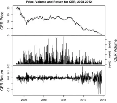
The data used in this paper are obtained from Thomson Reuters Point Carbon, a provider of independent news, analysis, and consulting services for European and global power, gas, and carbon markets. Access to this data requires paid membership. We focus on price and trade volume for both EUA and CER between June 2008 and December 2012. For both assets, price, trade volume, and log-return series are given in Figures 1 and 2. The dynamics of the carbon market as discussed in the previous section are clearly reflected in these figures. In particular, we observe a high market in both EUA and CER prices in the beginning of 2008–2012 period, followed by a steady decline and high volatility in the log-return series of both commodities in the second half of the period. The EUA and CER volume series behave somewhat differently. It is observed that EUA trade volumes show a more steady behavior throughout the entire period, where the CER volumes show higher averages and more variability in the first half. Autocorrelation functions and Q–Q normality plots for log-returns are provided in Figures 3 and 4. We observe from Figure 3 that the EUA returns show low correlations in the earlier lags and higher autocorrelations for higher lags, indicating a long-range dependence. Also, the Q–Q plots point to non-normality in the tails. Figure 4, on the other hand, indicates autocorrelations both in smaller and larger lags, showing a stronger evidence for long-range dependence. We also present the some descriptive statistics of the data in Table I, and correlations among the series in Table II.
As mentioned in the preceding text, the autocorrelation functions of the data indicate long-range dependence as a first sign. Formally, a stationary sequence is said to exhibit long-range dependence if its auto covariance function𝛾 tends to 0 so slowly that∑k=∞k=−∞𝛾(k) diverges (Samorodnitsky and Taqqu [25, pg.335]). This amounts to long-term correlations across arbitrarily large time lags. Our analysis in the next section shows that an asymptotic power-law behavior holds at least in some parts of the data. Therefore, the autocorrelation functions of the log-returns are not summable, and they are long-range dependent. Moreover, a self-similarity characteristic, which is defined as the compensation of a scaling in time by a scaling in space, can also accompany long-range dependence in data. This property appears as burstiness over a wide range
Figure 1.Price, volume, and return series for EUA, 2008–2012.
Figure 2.Price, volume, and return series for CER, 2008–2012.
of timescales. The search for long-range dependence and heavy-tails in financial data has been of interest, for example, Cont [26]. In particular, it is reported that 2005–2006 emission allowance prices are non-stationary, which they exhibit abrupt discontinuous shifts, and the distribution of the logarithmic returns is non-normal with heavy tails (Daskalakis et al. [11]). Several approaches for modeling the returns of emission allowances in this period are investigated in Benz and Truck [21], and the use of Markov switching and AR–GARCH models is suggested. Geometric Brownian motion and mean reverting square-root process, both with added jumps, have been found to fit best to the 2005–2006 data. Although jumps are reported to account for volatility in the data, these diffusion models are Markovian and do not capture long-range dependence. Therefore, we use fractional fBm as a continuous-time model with both long-long-range dependence and self-similarity.
Because the observed-price series are discrete time processes, we also considered ARMA and GARCH models, which are versatile tools commonly employed for the analysis of time series data. These models have become important in the analysis of time series data, particularly in financial applications. The ARMA specification is usually employed for modeling conditional mean, and GARCH models proved to be useful for modeling non-constant variance in the series.
Figure 3.Autocorrelation function and normality plot for European Union Allowance returns.
Figure 4.Autocorrelation function and normality plot for CER returns.
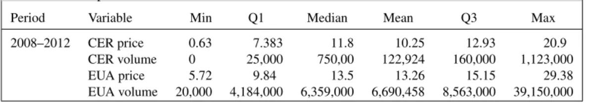
Table I.Descriptive statistics for EUA and CER.
Period Variable Min Q1 Median Mean Q3 Max
2008–2012 CER price 0.63 7.383 11.8 10.25 12.93 20.9
CER volume 0 25,000 750,00 122,924 160,000 1,123,000
EUA price 5.72 9.84 13.5 13.26 15.15 29.38
EUA volume 20,000 4,184,000 6,359,000 6,690,458 8,563,000 39,150,000 EUA, European Union Allowance.
Table II.Correlation matrices.
Period CER price CER volume EUA price EUA volume
2008–2012 CER price 1 0.097 0.958 −0.069
CER volume 1 0.052 −0.003
EUA price 1 −0.102
EUA volume 1
EUA, European Union Allowance.
Because the introduction of ARMA models in 1982 by Engle and the GARCH models in 1986 by Bollersev, these models have been intensively studied in the literature. Hence, we do not further elaborate on them here but present the particular models that we have used in Section 4. In the rest of our study, we refer to these models as ARMA–GARCH models.
3. Continuous time modeling of European Union Allowance and CER prices
In this section, we fit fBm to log-return data and compare with mean reverting process as a benchmark model. 3.1. Fractional Brownian motion
We begin with a brief description of the model. A fBm BH with Hurst parameter H ∈ (0, 1) is a Gaussian process with
covariance function
Cov(BHs, BHt )=1 2 [
t2H+ s2H−|t − s|2H] .
It was first introduced by Mandelbrot and van Ness [27] and has found applications in various fields. The increments of fBm over unit time intervals are called fractional Gaussian noise (fGn) ([25]). When we consider increments of one unit of time, the autocovariance function of fGn is found as
𝛾(k) ∶= E[BH1 (BHk+1− BHk)]
= E[BH1BHk+1− BH1BHk]= (k + 1)
2H+ (k − 1)2H− 2k2H
2 .
It follows that fGn is a stationary Gaussian process, and 𝛾(k) = 1
2 [
2H (2H − 1) k2H−2+ O(k2H−4)] (1)
by a binomial expansion for large k values. As a result,𝛾(k) ∝ k2H−2and it is not summable, that is∑k=∞
k=−∞𝛾(k) diverges,
when 1∕2< H < 1. For these values of H, fGn is called long-range dependent. This property is also said to hold for the original process, namely, fBm. Note that the autocovariance function of a long-range dependent process has a slow power-like decay, while that of a Markovian process decays exponentially. Higher H values indicate stronger dependence. For H = 1∕2, fBm simply reduces to a Brownian motion.
In our analysis, we model the price series Pt, t = 1, 2, … with mean parameter 𝜇 and variance parameter 𝜎 > 0 by
Pt = P0e𝜇t+𝜎BHt, (2)
which is called a geometric fBm. Accordingly, the logarithmic return series is given by
Xt = log Pt− log Pt−1=𝜇 + 𝜎(BHt − BHt−1), (3) t = 1, 2, …, and involves fGn.
First of all, we have studied if there is any seasonality in the logarithmic returns which are expected to form a stationary process. In view of general linear model (GLM procedure) implemented in SAS, we have not observed a significant effect of days and months, or their interaction on the mean with p-values 0.433, 0.046, and 0.629, respectively. Although 0.046 is somewhat low, the effect is not highly significant. Therefore, any effect of the months is also assumed to be negligible. 3.2. Model fit with fBm
In this section, we fit the parameters of an fBm model to EUA and CER series. All calculations are carried out in MATLAB with our codes of the relevant algorithms and those available in [28].
3.2.1. Change-point analysis. We first search for the the change-points in data as indicated by the change-points in the parameters of the fBm model (3). The Hurst parameter H determines the autocorrelation structure of the data. Therefore, a method based on locating the variance change-point has been proposed for a fractal time series such as fBm in Rincon and Sallent [29]. It is based on the wavelet transform of the data so that a less correlated series is obtained. Then, the variance of the transformed data is monitored for a change-point using Schwarz information criterion (SIC) as developed by Chen and Gupta [30]. Multiple variance change-points can be located by performing the same analysis on the subparts found after the first change-point, and continuing in this manner on further subparts.
We have chosen the method of Rincon and Sallent [29], as it is based on a well-studied theory for Gaussian series, for example, the asymptotic analysis of the statistic based on SIC is available with critical values for determining the statistical significance [30]. It is applicable to the wavelet transform of fBm, which is also Gaussian. Moreover, this approach is in
accordance with the method we use in the succeeding text for estimating the parameters of fBm, as both methods benefit from wavelet transform to exhibit superior properties. Discrete wavelet transform is also proposed in Zuraniewski [31] in combination with SIC for Hurst parameter change-point detection. Another statistic is analyzed in Chatterjee et al. [32], again based on discrete wavelet transform for variance change-point.
The change-points in the transformed data indicate regions in the original sequence where the change may have occurred. If this happens around the same region in sufficient number of resolution levels corresponding to wavelet analysis, we consider the union of these regions and report the mid-point. The first change-point for EUA series occurs around mid-May 2009. After applying the method to the first and second parts separately, we detect another change-point at the beginning of September 2011 in the second part. There remains no change-points in the series at a significance level of 0.10, which is chosen to be not so small as to capture all the points. As a result, the EUA series is split into three pieces as also visually anticipated from Figure 1 (these change-points are indicated as vertical lines in Figure 8). On the other hand, the CER series mostly behaves like EUA except for the final part. Three significant change-points are detected in mid-May 2009, mid-September 2011, and at the end of August 2012 when the certificate is close to its expiration in December 2012. The resulting four segments are also indicated by the vertical lines in Figure 2. We will interpret these regions in connection with the parameter estimates below.
3.2.2. Parameter estimates. We use the Abry–Veitch estimator derived in Veitch and Abry [33] for estimating the Hurst parameter. The method is based on the wavelet transform of the data. There are also other methods for Hurst parameter estimation. In Jeong et al. [34], various estimators are compared on the basis of simulated fGn. When compared with most methods used, the wavelet method emerges as an unbiased and half parametric method that is adequate to estimate the Hurst parameter. The Whittle estimator with a similar performance is also unbiased, but the computations are heavier, and it depends on the Gaussian distribution hypothesis.
In Veitch and Abry [33], stationary processes with autocovariance function satisfying
𝛾(k) ∼ c𝛾k−(1−𝛼), (4)
as k→ ∞, where c𝛾> 0, 0 < 𝛼 < 1, are considered. The range of values of the parameter 𝛼 implies long-range dependence for the process. In view of (1), long-range dependence parameter 𝛼 in (4) is a function of the Hurst parameter of fGn, given by
𝛼 = 2H − 1, and the coefficient is found as
c𝛾= 𝜎
2
22H (2H − 1).
The property (4) is equivalent to the condition that Fourier transform f of𝛾 satisfies f (𝜈) ∼ cf𝜈−𝛼,
when 𝜈 → 0 in the frequency space, where cf > 0. The estimation of these parameters is a difficult problem because the autocorrelation function decays slowly. Clearly, we do not have i.i.d data, which would yield nice properties for the estimator. Instead, the data are transformed by wavelets to take the autocorrelations into account and the estimator ̂cf is derived simultaneously with ̂𝛼 as Abry–Veitch estimators in [33].
In this section, using the estimate of cf and the relation
cf = 2(2𝜋)−𝛼c𝛾𝚪 (𝛼) sin((1 − 𝛼)𝜋∕2), (5)
we simply estimate the variance coefficient𝜎 as
̂𝜎 = √ √ √ √ (2𝜋)̂𝛼̂cf 2 ̂H(2 ̂H − 1)𝚪 (̂𝛼) sin((1 − ̂𝛼)𝜋∕2), where ̂H = (̂𝛼 + 1)∕2.
We apply the estimation method to EUA first, for which the price series and log-returns are given in Figure 1. The drivers of the eventual fall in prices might be the global financial crisis, and other market factors discussed in the first section, as well as the termination of the second stage of Kyoto Protocol that began in 2008. Because we have identified three different subseries, we estimate the parameters as given in Table III. The three periods indeed have different variance parameters as
Table III.Fractional Brownian motion parameter estimates for EUA series.
Period for EUA series ̂H and 95% CI ̂𝜎 ̂𝜇
6/12/2008 to 5/11/2009 0.662 [0.509, 0.816] 0.0336 −0.0027 5/12/2009 to 9/2/2011 0.532 [0.447, 0.617] 0.0172 −0.0003 9/3/2011 to 12/5/2012 0.496 [0.374, 0.618] 0.0375 −0.0022 EUA, European Union Allowance.
Table IV.Fractional Brownian motion parameter estimates for CER series.
Period for CER series ̂H and 95% CI ̂𝜎 ̂𝜇
8/12/2008 to 5/5/2009 0.765 [0.584, 0.947] 0.0368 −0.0028 5/6/2009 to 9/14/2011 0.540 [0.462, 0.619] 0.0155 −0.0005 9/15/2011 to 8/24/2012 0.538 [0.384, 0.693] 0.0428 −0.0051
indicated from either H and/or𝜎. We can conclude that the EUA prices have shown fluctuations with long-term correlations just after introducing the certificates in the market. In the first period, long-range dependence is observed with a Hurst parameter of 0.662, and 0.509 as the lower limit of the 95% confidence interval, and it is reasonable to model the prices with fBm. A Hurst parameter value around 0.6 is consistent with the previous studies of other price series as reported in [23, 24]. In mid-May 2009, the first regime change is observed to be a series having essentially no long-range dependence with H = 0.532. The second change-point is detected as September 2011, but mainly due to the variance coefficient 𝜎 rather than a significant change in H. Recall from (4) that the autocorrelation function is a function of both H and𝜎. To validate the model visually, we have also performed simulations of (2) and obtained random trajectories that are similar to real price data. We have also inspected the residuals, and the results are separately discussed in the succeeding text.
For CER, the price series and log-returns are plotted in Figure 2. The fBm parameter estimates are given in Table IV, according to which CER prices also show long-range dependence in the first period, from the beginning till mid-May 2009, as in the EUA series. The Hurst parameter estimate is 0.765, a higher value than H of EUA series. In the second and third periods, the Hurst parameter estimates are close to 1/2, and actually very close to each other as well. First, we conclude that a Brownian motion would fit well in these periods. Second, the fact that variance coefficient𝜎 is quite different must have led to a change-point in mid-September 2011 by our detection algorithm, rather than a change in H. In the fourth period covering August 24, 2012 to December 5, 2012, there are too few observations for a reliable estimation of the parameters by the wavelet method. In this period, the price basically vanishes as the term ends; hence, no results are reported.
Residual Analysis:
We analyze the residuals resulting from the fBm fit using the prediction formulas derived in Norros [35]. We use the conditional expectation
̂Xt+1= E[Xt+1|Xs, 0 < s ⩽ t] for prediction of the log-returns. By Eq. (3), we have
̂Xt+1=𝜇 + 𝜎 ̂dBt+1, (6)
where ̂dBt+1= E[Bt+1− Bt|Bs, 0 < s ⩽ t]. By using the differential equation satisfied by fBm ̂
dBt+1= ∫
t
0
gt(1, s) dBt−s (7)
is derived by Gripenberg and Norros [36] where
gt(a, s) = sin(𝜋 (H − 1∕2)) 𝜋 s−H+1∕2(t − s)−H+1∕2∫ a 0 rH−12(r + t)H−1∕2 r + s dr,
382
in particular a = 1 in our case. Numerical evaluations in [35] show that function g gives more weight to the very recent observations, and the effect of the past values decreases sharply. The prediction formula (7) becomes only a sum with our discrete data. Therefore, we scale the predicted values ̂dB to obtain a sequence with variance 1, before substituting it into Eq. (6).
For the EUA returns series with n = 1, 119 days, residual analysis is conducted as follows: For each period, the residuals Xt− ̂Xt,
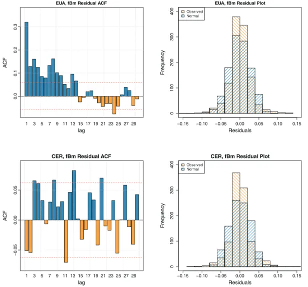
where Xt is the logarithmic return series given in (3), and ̂Xt is obtained from (6), are computed. We obtained residual sum of squares (RSS) = 0.8650661 and the mean equare error (MSE) = RSS/n = 0.000773. For the CER returns series n = 996 days (shorter because we did not fit a model to the very last part, where the series is diminishing) RSS is obtained as RSS = 0.7873647 and MSE = 0.000791. The autocorrelation functions and histograms of the residuals for EUA and CER series are given in Figure 5. Residual histograms are plotted against histograms of randomly generated samples from normal distributions with the same sample size, mean and standard deviation as the observed residuals. Although histograms and the autocorrelation functions visually indicate reasonably good fit of the fBm model, the formal Jarque– Bera [37] test for the normality of the residuals is rejected (p-value<2.2–16) for both the EUA and CER data. This may be attributed to a slight leptokurtic behavior of the residual histogram with a higher peak in the center and relatively thick on the tails compared with normal. We also note that because the sample sizes are quite large, even small shifts may lead to rejection of the hypothesis.
Figure 5.Autocorrelation functions (ACF) and residual histograms for European Union Allowance (EUA) and CER for the fractional Brownian motion (fBm) method.
3.3. Mean-reverting process as a benchmark
As a continuous-time benchmark model, a diffusion process can be considered as in [11]. A mean-reverting model is a promising candidate because the series seems to converge to a stationary regime after an oscillation. This is observed both in the beginning and towards the end of the trajectories. Therefore, we analyze the data in two halves. A mean reverting square-root process with jumps was found to fit best to the 2005–2006 emission allowance prices. Our analysis aims to compare a Markovian model with a long-range dependent model on the basis of goodness of fit. Therefore, we consider a mean-reverting process with no additional jumps as a basic model. Introducing jumps would be only fine-tuning, which is not necessary for comparison purposes. In Abadie and Chamorro [38], the authors used a mean-reverting model for electricity prices, which is not associated with EUA prices. They modeled the EUA prices with geometrical Brownian motion. On the other hand, the emission allowance is modeled with a mean-reverting, in particular, the Ornstein–Uhlenbeck process in Laurikka [39]. A related model for discrete time which is a special AR(1) process is used in Benz and Truck [21] where two regimes are mentioned.
The mean-reverting model is expressed by the Ito differential equation
dPt=𝜂(𝜇 − Pt)dt +𝜎dBt (8)
where𝜂 is a parameter that determines the rate of reversion to the mean, and 𝜇 and 𝜎 are directly equal to the mean price and variance parameters, respectively (e.g., Oksendal [40]). It is a linear model, so (8) can be solved analytically. The solution is given by Pt= P0e−𝜂t+𝜇(1 − e−𝜂t)+𝜎e−𝜂t t ∫ 0 e𝜂sdBs. When t→ ∞, the price Ptconverges to𝜇.
The maximum likelihood method is used for parameter estimation using the following numerical approach: First𝜇 and𝜎 are expressed in terms of 𝜂 using the first order conditions. In this way, the numerical search is simplified because the likelihood function is expressed only in terms of 𝜂. Then, the maximization is performed over the single variable 𝜂 (Johnson and Barz [41], Franco [42, pg.4]) with MATLAB’s ‘fminsearch’ function, which is used in its default form without modifying its options. The parameters𝜇 and 𝜎 are estimated in turn. The results are given in Table V for the first and second half of both series.
According to the results given in Table V, EUA prices converge to 15.46, and CER prices converge to 12.99 in the first half. These two means are observed in Figures 1 and 2. On the other hand, prices tend to decline in the second half. For this part, the steady state EUA prices predicted in Table V is 10.22. The model predicts that even if the prices were below 10.22 at the end of 2012, it would fluctuate around 10.22 during that time. Similarly, it is predicted that CER in the second part converges to 6.61, which is higher than the observations. Therefore, the mean-reverting model is not considered appropriate for the second part of CER. We have studied the mean-reverting process (8) as a baseline diffusion model in comparison with fBm. However, the residuals are much higher. This is easy to see because it is a Markovian model that predicts the next days price only from todays price by
E[Pt+1|Pt] = e−𝜂Pt+𝜇(1 − e−𝜂).
Using the estimated values of𝜂, the predicted values are practically equal to mean 𝜇. Moreover, this model cannot capture long-range dependence, in contrast to fBm.
Table V.Parameter estimates for mean-reverting model.
EUA CER
2008–2010 2011–2012 2008–2010 2011–2012
𝜂 39.35 39.75 39.35 39.35
𝜇 15.46 10.22 12.99 6.61
𝜎 35.67 31.92 20.57 35.57
EUA, European Union Allowance.
4. Autoregressive moving average–generalized autoregressive conditional heteroskedastic
modeling of European Union Allowance and CER prices
In this section, we model the EUA and CER log-return series as univariate ARMA–GARCH processes, with trade volumes as potential covariates. In financial data, usually trade volume is not taken as a price determinant, but we wanted to inspect the trade volume effect. Because the carbon market is not a traditional market and because the ultimate idea is to reduce carbon emissions, this market could respond to trading volumes differently. All computations in this section are carried out with the rugarch package [43] for the statistical computing software R.
4.1. Autoregressive moving average–generalized autoregressive conditional heteroskedastic modeling
We model the time series of EUA and CER returns as univariate ARMA–GARCH processes, where the mean equations are assumed to be ARMA processes, and the innovations are assumed to be generated from GARCH processes. Consider a univariate time series Xt. The ARMA(m, n) process of autoregressive order m and moving average order n is given by
Xt=𝜇 + m ∑ i=1 aiXt−i+ n ∑ j=1 bj𝜖t−j+𝜖t, (9)
where𝜇 is the mean, ai(i=1,...,m) are autoregressive coefficients, bj(j =1,...,n) are the moving averages, and𝜖t are the innovations or residuals. The mean equation cannot take into account the typical features of financial data such as het-eroskedastic effects, volatility clustering, and leverage effect. In order to model such financial phenomena, Engle [44] introduced Autoregressive Conditional Heteroskedastic model (ARCH), which was later generalized by Bollerslev [45] and named Generalized Autoregressive Conditional Heteroskedastic model (GARCH). The innovations of the ARMA mean equation are often modeled with GARCH. The variance equation of the GARCH(p, q) model is given by
𝜖t = zt𝜎t, zt ∼ D𝜈(0, 1), 𝜎2 t = 𝜔 + k ∑ j=1 𝛾j𝜃jt+ p ∑ i=1 𝛼i𝜖2t−i+ q ∑ j=1 𝛽j𝜎t−j2 , (10)
where D𝜈 is the distribution of the innovations with zero mean and unit variance,𝜎2t is the conditional variance, 𝜔 is the intercept,𝜃j(j=1,...,k) are possible covariates (external regressors), and𝜖tare the residuals from the mean (filtration) process. In this study, we employ ARMA(m, n) models with innovations following GARCH(p, q) models, denoted by ARMA(m, n)–GARCH(p, q), with possible covariates.
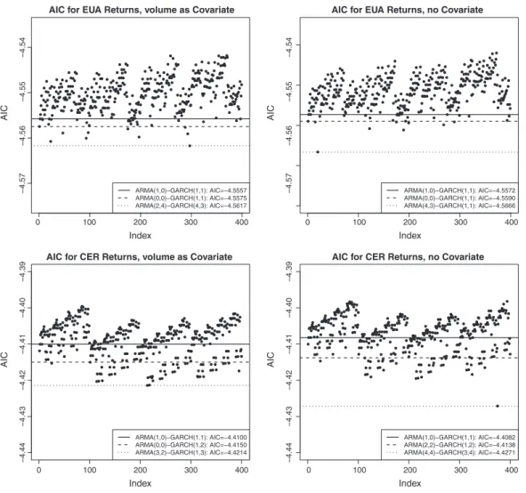
4.1.1. Model specification. In order to identify the best performing ARMA–GARCH models that explain the EUA and CER prices, we carried out an extensive search in this class, over the model parameters (m, n, p, q). In particular, the ARMA(m, n)–GARCH(p, q) models given in (9) and (10), where Xtis taken as the log-returns, that perform best in terms of the AIC criteria are investigated for the EUA and CER series over the period of 2008–2012. We conducted the search over the set 0 ⩽ m, n ⩽ 4 and 1 ⩽ p, q ⩽ 4, which resulted in a total of 25×16 = 400 alternative models for each of the two series. As both series are also considered with and without the volume series taken as a covariate, 1600 models in total are investigated in our search. We based our decision on the Akaike Information Criterion (AIC), a common criterion for comparing models, which seeks for balance between lack of fit and complexity of the models, small values of which imply a better performance. As a benchmark to our investigation, we used the results of Benz and Truck [21] who proposed to use AR(1,0)–GARCH(1,1) model to analyze the short term behavior of the EUA data over the period of 2005–2006. Because the number of investigated models are very large and the total number of estimated parameters can be as high as 16, we also were interested in the behavior of relatively simpler models, which we referred to as parsimonious models, where we restricted the (m, n, p, q) parameters to be less or equal to 2. Hence, we inspected the performances of 3×3×2×2 = 36 such models with relatively less number of parameters. The AIC values of the 400 models considered are given in Figure 6, where the AIC values of the best performing; the benchmark and the best parsimonious models are indicated by the horizontal lines. The top two figures refer to the results for the EUA returns, the left one with the sales volume taken as a covariate and the right one without the covariate. Similar figures for the CER returns are given in the bottom. We observe that the best parsimonious models perform better than the benchmark in all four cases, and the best model results in a significantly lower
Figure 6.Plots of the search for autoregressive moving average (ARMA)(m,n)–generalized autoregressive conditional heteroskedas-tic(p,q) models. European Union Allowance (EUA) and CER returns studied with and without trade volume as a covariate. Top
models, top parsimonious models, and the benchmark models are indicated with horizontal lines.
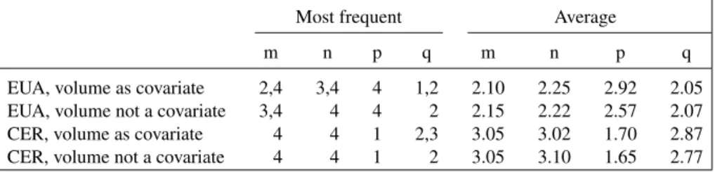
AIC value, especially in the CER data with no covariate. For both the EUA and CER prices, the best performing ARMA– GARCH models with parameters (4,3,1,1) and (4,4,3,4), respectively, turned to yield a better performance when the sales volume is not taken as a covariate. Notice however that for the CER data, both the benchmark model with parameters (1,0,1,1) and the most parsimonious model with parameters (0,0,1,2) have a better performance when sales volume data is in the model. This may suggest that, when simpler models are used additional information provided by the sales volume data may be helpful to improve the model performance, whereas this advantage disappears as more complicated models are employed, that is with increased number of parameters further information on the sales volume may become redundant. Because a large number of models have been inspected, some other features of the results would also be of interest. In Table VI, we present the most frequently occurring and the average (m, n, p, q) values of the top %10 of the models which may give a quick idea about the values that these parameters assume for reasonably good models. As it obviously makes more sense to capture the joint behavior of these parameters, we provide the results for the three best ARMA–GARCH models, three best performing parsimonious models and the benchmark models, together with their AIC values and the overall rankings in Table VII. From this table, we observe that the best parsimonious model performs notably well for the EUA data with a ranking of 10 and 9 out of 400 models, and the ranking of the benchmark model is quite reasonable with corresponding values of 32 and 26. For the CER data, the rankings deteriorate somewhat and drop to 55 and 48 for the parsimonious models in models with and without the covariate respectively and to 145 and 150 for the benchmark models. 4.1.2. Rolling estimation. Another interesting question is the stability of the underlying ARMA–GARCH models over the time span of 2008–2012. The initial inspection of the observed series pointed to possible structural changes in the data over the considered time interval. To investigate for further evidence on this issue, we considered a rolling estimation of the
Table VI.Most frequent and Average m,n,p,q values for the best % 10 of the models.
Most frequent Average
m n p q m n p q
EUA, volume as covariate 2,4 3,4 4 1,2 2.10 2.25 2.92 2.05
EUA, volume not a covariate 3,4 4 4 2 2.15 2.22 2.57 2.07
CER, volume as covariate 4 4 1 2,3 3.05 3.02 1.70 2.87
CER, volume not a covariate 4 4 1 2 3.05 3.10 1.65 2.77
EUA, European Union Allowance.
Table VII.Summary of the search for ARMA(m,n)–GARCH(p,q) models. EUA and CER returns studied with and without trade volume as a covariate.
m n p q AIC Rank
EUA, volume Top 2 4 4 3 −4.5617 1
as covariate 2 4 1 1 −4.5608 2 3 3 4 1 −4.5601 3 Top parsimonious 0 0 1 1 −4.5575 10 1 1 1 1 −4.5560 25 0 1 1 1 −4.5558 29 Benchmark 1 0 1 1 −4.5558 32
EUA, volume Top 4 3 1 1 −4.5666 1
not a covariate 4 2 4 2 −4.5611 2 2 4 1 2 −4.5608 3 Top parsimonious 0 0 1 1 −4.5590 9 0 1 1 1 −4.5573 25 1 0 1 1 −4.5573 26 Benchmark 1 0 1 1 −4.5573 26
CER, volume Top 3 2 1 3 −4.4214 1
as covariate 2 3 1 3 −4.4213 2 3 2 1 2 −4.4203 3 Top parsimonious 0 0 1 2 −4.4150 55 2 2 1 2 −4.4143 65 2 2 2 2 −4.4133 82 Benchmark 1 0 1 1 −4.4100 145
CER, volume Top 4 4 3 4 −4.4271 1
not a covariate 3 2 1 3 −4.4195 2 2 3 1 3 −4.4194 3 Top parsimonious 2 2 1 2 −4.4138 48 0 0 1 2 −4.4128 64 1 0 1 2 −4.4111 85 Benchmark 1 0 1 1 −4.4082 150
Top three models, top three parsimonious models, and the benchmark models are reported. The best models among the considered ones are given in boldface. ARMA, autoregressive moving average; GARCH, generalized autoregressive con-ditional heteroskedastic; EUA, European Union Allowance.
parameters. Commonly used as a backtest of a statistical model on historical data, a rolling estimation procedure computes the parameter estimates over a rolling window of a fixed size through the sample. If the parameters change at some points, the rolling estimation captures these structural changes. We applied rolling estimation with the best fitting models discussed previously. For illustrative purposes, we only present the results for the EUA data with the ARMA(4,3)–GARCH(1,1) model with no covariate. In the rolling estimation, we used the first 120 days as the training period which corresponds to a 6 months data because weekends are excluded, from which the initial estimates of the model parameters are obtained. Then, one-step ahead predictions using these parameters are carried out for the next 60 days that corresponds to a quarter of a year. After 60 days, the model parameters are re-estimated, based on the most recent 120 days, that is, days 61–180.
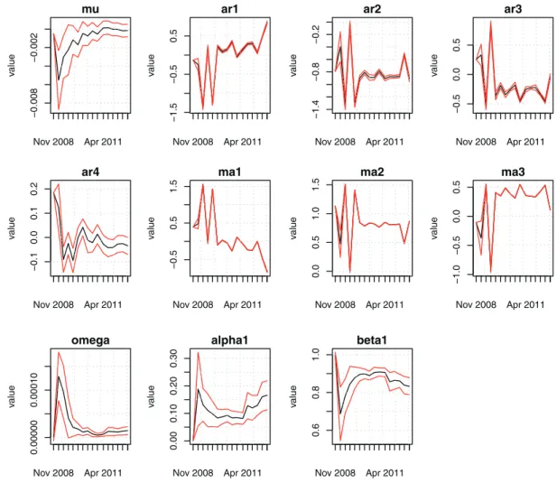
Figure 7.Evolution of autoregressive moving average(4,3)–generalized autoregressive conditional heteroskedastic(1,1) parameters in the 16 fits of the rolling estimation for European Union Allowance returns.
This procedure continues in this rolling window manner until the end of the available data range. The results are given in Figure 7. As the parameter estimates are updated every 60 days, we have a total of 16 estimates for each parameter which are plotted in the figure. Because Figure 7 was automatically generated by the rugarch package of R, we were unable to use the parameter names introduced in Section 4.1. Note here that in these plots the parameters mu, ar1, ar2, ar3, ar4, ma1,
ma2, ma3 correspond to𝜇, a1, a2, a3, a4, b1, b2, b3; and omega, alpha1, beta1 correspond to𝜔, 𝛼1,𝛽1, respectively. A common feature for all parameter estimates is that almost all of them indicate a changing behavior. After an initial drop, the
muvalue shows a steady increase in the first half and then stabilizes more in the second half. Some of the other estimates such as ar1, ma1, and alpha1 present a change both in the level and in the variability, whereas the parameters omega and beta1 show more variability in the beginning but then stabilize in the second half. These observations indicate that highly sophisticated factors play roles in the determination of the prices. The changes in the parameter estimates mentioned previously motivated us to carry out a more detailed change-point analysis to identify the possible structural changes in the model.
4.2. Change-point analysis
Consider an observed univariate time series x1∶N = (x1, ..., xN). A change-point is said to occur if there exists a time 𝜏 ∈ {1, ..., N − 1} such that statistical properties of {x1, ..., x𝜏} and {x𝜏+1, ..., xN} are different in some way. Generalizing to
multiple change-points, we denote the r change-points by𝜏1∶r = (𝜏1, ..., 𝜏r), where 1< 𝜏1 < 𝜏1 < ...𝜏r< N. Consequently, r change-points will split the data into r+1 sub-series. Our purpose is to estimate the unknown ARMA–GARCH parameters along with the change-points, based on N observations. For the estimation procedure, we used time series methods where dummy variables taking values one or zero are used to indicate within which sub-series an observed value falls. Hence, if there are r change-points, there will be r dummy variables to characterize the sub-series, where all the dummies being
zero indicates that the observation is in the (r + 1)st sub-series. Let M𝜏
1∶rdenote the ARMA–GARCH model with a given
set of orders (m, n, p, q), and given covariates 𝜃. Let AIC(M𝜏
1∶r) denote the AIC obtained when M𝜏1∶r is fitted to the data.
The estimated change-point set will be the set that minimizes the AIC criteria, that is,
̂𝜏1∶r = argmin𝜏1∶rAIC(M𝜏1∶r). (11)
The search for the minimizing set also returns the possible change-points together with the corresponding parameter esti-mates of the ARMA–GARCH model that minimizes the AIC criteria. Although this approach is standard and conceptually straightforward, it rapidly becomes computationally prohibitive when all possible choices for all r values are considered. In order to shrink the search space, we referred to the results of the change-point analysis of Section 3. In particular, we focused only on the candidate change-points that lie over a reasonably large interval constructed around the change-points suggested by the fBm analysis. For the three ARMA–GARCH models discussed earlier (the best performing, the best parsimonious and the benchmark models), the estimates for the change-points and the ARMA–GARCH parameters are obtained by the minimization given in (11). The results of this approach will be referred to as Search Based (̂𝜏) in the following discussion. For comparison purposes, we also present two other results obtained by fitting the ARMA–GARCH models with fixed change-points suggested by (i) the midpoints of the intervals obtained by the fBm analysis and (ii) the change-points suggested by the PELT algorithm, referred to as Mid Point and PELT, respectively. The PELT (Pruned Exact Linear Time) algorithm is a recent method for detecting multiple change-points in a time series. A common approach in change-point literature is to minimize a cost function for a segment, and at the same time, minimize a penalty term to guard against overfitting. Once the cost and penalty terms are selected, one of the iterative search algorithms, such as binary segmentation, segment neighborhood, or optimal partitioning methods, can be used. The PELT method aims to increase the computational efficiency of the optimal partitioning method by pruning some of the iteration paths, that is, removing those values of change-point candidates that can never be a minima for the minimization performed at each iteration. Proposed by Kilick et al. [46], the PELT algorithm assumes normality of data points and returns change-points which minimize the cost and penalty functions mentioned previously. Changing a tuning parameter sets the number of change-points estimated by this algorithm.
4.2.1. Change-point analysis of EUA returns. According to the fBm analysis, EUA returns exhibit two structural changes, the first one in mid-May 2009, and the second at the beginning of September 2011. We used this result as a basis to reduce the search efforts in the point analysis presented in the preceding text. In particular, we focused on the change-point alternatives𝜏1∶2= (𝜏1, 𝜏2), where𝜏1varies between February 24 and July 17 of 2009 (days 180 and 280 of our data
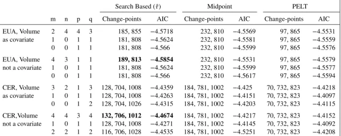
Table VIII.Change-point search results for the considered ARMA(m,n)–GARCH(p,q) models. EUA and CER returns studied with and without trade volume as a covariate.
Search Based(̂𝜏) Midpoint PELT
m n p q Change-points AIC Change-points AIC Change-points AIC
EUA, Volume 2 4 4 3 185, 855 −4.5718 232, 810 −4.5569 97, 865 −4.5531 as covariate 1 0 1 1 181, 808 −4.5624 232, 810 −4.5581 97, 865 −4.5559 0 0 1 1 181, 808 −4.566 232, 810 −4.5599 97, 865 −4.5576 EUA, Volume 4 3 1 1 189, 813 −4.5854 232, 810 −4.5531 97, 865 −4.5579 not a covariate 1 0 1 1 181, 808 −4.5624 232, 810 −4.5599 97, 865 −4.5577 0 0 1 1 181, 808 −4.566 232, 810 −4.5617 97, 865 −4.5594 CER, Volume 3 2 1 3 128, 704, 1008 −4.4359 184, 781, 1002 −4.425 70, 732, 823 −4.4218 as covariate 1 0 1 1 128, 704, 1008 −4.4263 184, 781, 1002 −4.4151 70, 732, 823 −4.4097 0 0 1 2 128, 704, 1026 −4.4315 184, 781, 1002 −4.4203 70, 732, 823 −4.4115 CER,Volume 4 4 3 4 132, 706, 1012 −4.4674 184, 781, 1002 −4.4217 70, 732, 823 −4.4152 not a covariate 1 0 1 1 128, 704, 1008 −4.4271 184, 781, 1002 −4.4145 70, 732, 823 −4.4092 2 2 1 2 116, 706, 1028 −4.4535 184, 781, 1002 −4.5251 70, 732, 823 −4.4208
Change-points estimated by the search based algorithm(̂𝜏) for the best, best parsimonious, and benchmark ARMA–GARCH models are indicated. Change-points suggested by the fBm analysis (Midpoint) and the PELT algorithm are also included in the table. Models with the lowest AIC are given in boldface.
ARMA, autoregressive moving average; GARCH, generalized autoregressive conditional heteroskedastic; EUA, European Union Allowance; PELT, pruned exact linear time; fBm, fractional Brownian motion.
Table IX.Descriptive statistics for EUA and CER in different segments.
Variable Min Q1 Median Mean Q3 Max
EUA Segment 1 Price 8.00 14.75 19.65 19.01 24.30 29.38
Volume 100,000 4,375,000 6,600,000 6,827,126 8,900,000 20,659,000
EUA Segment 2 Price 10.10 13.10 14.29 14.18 15.13 16.94
Volume 20,000 4,136,000 6,074,500 6,624,081 8,720,000 20,071,000
EUA Segment 3 Price 5.98 6.93 7.60 8.01 8.48 12.27
Volume 261,000 3,904,000 6,077,000 6,748,513 8,636,500 39,150,000
CER Segment 1 Price 7.60 12.82 15.11 15.20 19.00 20.90
Volume 0 10,000 36,000 89,875 112,250 548,000
CER Segment 2 Price 9.25 11.75 12.35 12.36 13.02 14.59
Volume 0 43,250 100,000 160,555 215,000 1,123,000
CER Segment 3 Price 2.40 3.78 4.48 5.85 8.09 12.53
Volume 0 21,750 55,000 83,246 111,750 575,000
CER Segment 4 Price 0.63 0.89 1.12 1.31 1.75 2.43
Volume 0 10,000 29,000 41,367 60,000 173,000
EUA, European Union Allowance.
Figure 8.Change-point estimates for European Union Allowance (EUA) and CER series based on search based, midpoint, and pruned exact linear time algorithm (PELT) approaches.
set), and𝜏2varies between June 24 and November 11 of 2011 (days 760 and 860 of our data set). The results are given in the first six rows of Table VIII, which correspond to the best, best parsimonious and the benchmark models with and without the covariates. We observe that the change-points suggested by the three methods differ notably and in terms of the corresponding AIC values, search-based models are the best ones, followed in general by the midpoint and then the PELT based models. The best performance is obtained by the ARMA(4,3)–GARCH(1,1) model with no covariate, and the model where sales volume is included as a covariate performs better only in the midpoint alternative with the best ARMA– GARCH model. The best performing ARMA(4,3)–GARCH(1,1) model suggests change-points at the days 189 and 813, which correspond to March 9, 2009 and September 7, 2011. This model splits the time span of 2008–2012 to three segments where the underlying models may have structural changes. The basic descriptive statistics for each segment are given in Table IX where notably different values for all measures are observed over different segments. Comparing these quantities with those in Table I that gives similar statistics for the entire data also reveal significant differences, which justifies the search for structural changes. The change-points returned by all three methods considered are given in Figure 8. Finally, we provide the estimated parameters of this model in Table X.
4.2.2. Change-point analysis of CER returns. According to the fBm method, CER return series exhibit three structural changes reported to be in mid-May 2009, in mid-September 2011, and at the end of August 2012. Similar to the analysis for the EUA returns, we only focus on candidate change-points𝜏1∶3 = (𝜏1, 𝜏2, 𝜏3), where𝜏1varies between January 5 and May 28 of 2009 (days 100 and 200 of our data set),𝜏2varies between April 27 and October 12 of 2011 (days 680 and 800), and𝜏3varies between July 12 and October 10 of 2012 (days 970 and 1,030). The results are given in the last six rows of Table VIII. We observe for this series also that the lowest AIC values are attained by the search based method, followed by the midpoint, and then the PELT algorithm. The best performing model appeared to be the ARMA(4,4)–GARCH (3,4) model without the covariate. We note however that the midpoint approach and the PELT algorithm result in better models with the sales volume as covariate with the best ARMA–GARCH and the benchmark models. The change-points that the best performing model indicates are at the 132, 706, and the 1,012 days, corresponding to February 24, 2009, June 2, 2011, and September 6, 2012. The basic statistics for the four segments implied by the previous change-points are given in Table IX. For this series also, we observe that there are notable differences in the values of all measures across the four segments. The change-points returned by all three methods considered are given in Figure 8. Comparison with the
Table X.Parameter estimates of the best ARMA–GARCH models among the considered ones, for EUA and CER.
EUA, ARMA(4,3)–GARCH(1,1) CER, ARMA(4,4)–GARCH(3,4)
with change-point dummies with change-point dummies
Estimate p-value Estimate p-value
𝜇 −0.0067 0.000 𝜇 −0.0039 0.000 a1 1.7869 0.000 a1 −0.1051 0.000 a2 −0.7158 0.000 a2 −0.0494 0.000 a3 −0.0086 0.000 a3 −0.0172 0.000 a4 −0.0929 0.000 a4 0.9528 0.000 b1 −1.8346 0.000 b1 0.0437 0.000 b2 0.7019 0.000 b2 −0.0048 0.000 b3 0.1585 0.000 b3 −0.0415 0.000 𝛾1 0.0073 0.000 b4 −1.0303 0.000 𝛾2 0.0048 0.001 𝛾1 0.0038 0.000 𝜔 0.00001 0.000 𝛾2 −0.0018 0.000 𝛼1 0.1666 0.000 𝛾3 −0.018 0.000 𝛽1 0.8304 0.000 𝜔 0.000 0.0745 𝛼1 0.2151 0.000 𝛼2 0.0257 0.861 𝛼3 0.000002 0.999 𝛽1 0.2183 0.737 𝛽2 0.0422 0.866 𝛽3 0.0474 0.738 𝛽4 0.4502 0.072
ARMA, autoregressive moving average; GARCH, generalized autoregres-sive conditional heteroskedastic; EUA, European Union Allowance.
Figure 9.Autocorrelation functions (ACF) and residual histograms for European Union Allowance (EUA) and CER for the autore-gressive moving average– generalized autoreautore-gressive conditional heteroskedastic (ARMA–GARCH) method. Presented are the best
(minimum AIC) among the considered models.
corresponding measures in the entire data given in Table I again point to the appropriateness of change-point models. The estimated parameters of the best performing model are given in Table X.
Residual Analysis
As a final point, we wanted to inspect the residuals of the models suggested by the ARMA–GARCH fitting. The plots of the ACF and histogram of the residuals from the best fitting ARMA–GARCH models for both the EUA and the CER series are given in Figure 9. For comparison purposes, the histogram of a normal sample with the same sample size, mean, and variance obtained from the observed data is also given on the same graph. The histograms and the autocorrelation functions indicate a reasonable fit to normally distributed error terms, although the variance of the residuals seem to be less than that of the normal sample, which may indicate an overfitting with the best performing ARMA–GARCH model. The formal Jarque–Bera [37] test for the normality of the residuals for the EUA and CER series are also rejected (p-values 8.5e-06 and< 2.2e-16 respectively), possibly due to the higher peak in the center and smaller variance compared with a normal distribution.
5. Discussion
European Union Allowance and CER price and return series are analyzed using both a continuous time stochastic process (fBm) and the time series (ARMA–GARCH) models. It is observed that the two analysis approaches provided comparable results, and their performances were superior compared with the benchmark counterparts. As for the interpretation of our
findings with respect to the global economic state, we observe that the period of interest in our analysis coincides with the global financial crisis starting in August 2007, with re-evaluation of the derivative instruments primarily specializing in the US mortgage markets. In May 2008, the weaknesses in the real estate and financial sectors in the USA became apparent with the release of the ‘stress tests’ results on the large banks and the reported losses of Fannie Mae and Freddie Mac, resulting in their being taken into receivership and the Lehman bankruptcy later in the year. To prevent a domino effect, western governments were obliged to inject vast sums of capital into their banks, culminating in a global decrease in credit flows and a recession. In late 2008, interest rates were cut drastically, and fiscal stimulus packages of varying sizes were announced, including quantitative easing. A further policy development occurred at the London G20 summit on April 2, 2009, when world leaders committed themselves to a fiscal expansion. In our analysis, such developments are indicated in the change-points observed in May 2009 for the EUA and CER prices captured by fBm analysis, and in March 2009 for EUA, and in February 2009 for CER indicated by the ARMA–GARCH models. By the end of 2010, the issue was no longer the solvency of banks but the solvency of governments. In May 2011, the US debt ceiling was reached (May 11), and Portugal’s rescue plan was approved (May 16). In September 2011, the second Greek bailout and austerity program ran into difficulties, resulting in government crises, and Italy passed its second austerity package (September 14), causing a revising-down of its credit ratings (September 16). The fBm analysis indicates changes in the beginning and middle of September of 2011 for the EUA and CER prices, respectively, whereas the ARMA-GARCH model captures changes for both the EUA and CER series in September of 2011. The last change in CER prices observed in August 2012 by fBm and in September by the ARMA–GARCH seems to be primarily due to the expiration in December of that year, but also the impact of the difficulties arising from the Greek debt crisis should not be overlooked.
6. Conclusion
In this work, the EUA and CER prices in the EU-ETS carbon market are studied during 2008–2012 period. Both stochastic and time series modeling of the market data obtained from Point Carbon company are considered.
Different from previous studies on stochastic models for price series, long-range dependence is analyzed in our work, using fractional Brownian motion. Mean reverting behavior is also investigated, which is not supported by the data. Initial analyses pointed to a possible change in the underlying models over the observation period. Hence, change-point detection is performed using data-driven approaches to identify the change-points where structural changes may come into play. The fBm analysis indicated that the EUA prices may have structural changes in May of 2009 and September of 2011, whereas CER prices indicate changes at mid-May of 2009, mid-September of 2011 and the end of August 2012.
Time series models are also employed for the analysis of the data. In particular, ARMA–GARCH models are used, where transactions volume is considered as a covariate. An extensive search is made over 400 models to determine the (m, n, p, q) parameters of the ARMA(m, n)–GARCH (p, q) models. Rolling horizon estimates of these parameters for the best fitting model supported evidence for several changes in the estimated parameters. Possible change-points are investigated using data-driven methods. In particular, a search based method is used to find possible change-points over intervals indicated by the fBm analysis. The results are compared to those provided by two other approaches based on fixed change-points proposed by the fBm method and the PELT algorithm. Obtained by the search based method, the best fitting model for the EUA series appeared to be an ARMA(4, 3)–GARCH (1, 1) model with two change-point dummy variables as covariates. Obtained similarly, the best fitting model for the CER series appeared to be an ARMA(4, 4)–GARCH (3, 4) model with three change-point dummy variables as covariates. Results for parsimonious models and a benchmark model are also provided. The change-points indicated by the ARMA–GARCH model were in March 2009 and September 2011 for the EUA series and in February 2009, June 2011, and September 2012 for the CER series.
The change-points indicated by both analysis methods are observed to parallel the global economic events as well, as discussed in the previous section. Although the global economic, political, and natural states have significant impacts on the prices of carbon related trade units in EU-ETS, our study shows that both fBm and time series models proved to be useful tools to uncover many properties of the price series as illustrated for the particular EUA and CER prices considered in our study. The behavior of the carbon markets in the third phase of EU-ETS, running from 2013 to 2020, is yet to be seen. However, it is not hard to say that this new stage introduces new challenges to the market and its researchers, as the regulations differ significantly from previous stages. We believe that the approaches provided in our work will also be useful to analyze and compare the the market specifics of EU-ETS in the coming phases.
Acknowledgement
This work is partially funded by the TUBITAK 110M307 research grant.