The expressive power of temporal relational query languages

The Expressive Power

of Temporal Relational Query Languages

Abdullah Uz Tansel, Member, IEEE Computer Society, and

Erkan Tin, Student Member, IEEE Computer Society

Abstract—We consider the representation of temporal data based on tuple and attribute timestamping. We identify the

requirements in modeling temporal data and elaborate on their implications in the expressive power of temporal query languages. We introduce a temporal relational data model where N1NF relations and attribute timestamping are used and one level of nesting is allowed. For this model, a nested relational tuple calculus (NTC) is defined. We follow a comparative approach in evaluating the expressive power of temporal query languages, using NTC as a metric and comparing it with the existing temporal query languages. We prove that NTC subsumes the expressive power of these query languages. We also demonstrate how various temporal relational models can be obtained from our temporal relations by NTC and give equivalent NTC expressions for their languages. Furthermore, we show the equivalence of intervals and temporal elements (sets) as timestamps in our model.

Index Terms—Attribute timestamping, expressive power of temporal query languages, N1NF relations, temporal relational algebra,

temporal relational calculus, temporal relational completeness, temporal relations, tuple timestamping. —————————— ✦ ——————————

1 I

HERE is a growing interest in temporal databases. This is because many applications require information not only about the present but also about the past. An object’s attributes may assume different values over time. The set of these values forms the history of that object. A temporal da-tabase (TDB) is thus defined as a dada-tabase that maintains object histories, i.e., past, present, and possibly future data.

Maintaining temporal data within a traditional relational database is not a straightforward endeavor. There are is-sues peculiar to temporal data, such as comparing database states at two different time points, capturing the periods for concurrent events and accessing times beyond these con-current periods, representing and restructuring temporal data, etc. These issues form the basis for the diversity in this field, which has been manifested by more than a dozen temporal relational data models and query languages pro-posed to date [1]. We believe that this diversity has helped delineate the issues in modeling and querying temporal data and has paved the way to explore the expressive power of the temporal relational query languages.

A comprehensive treatment of various approaches for handling temporal data is provided in [2]. A recent work-shop was dedicated to the establishment of an infrastruc-ture for temporal databases [3]. Data modeling, query lan-guages, standardization, and implementation issues were discussed. An outgrowth of this workshop has been an

ef-fort to design a temporal extension to SQL-92, called TSQL2. The design of TSQL2 has been completed, and its full specification is reported in [4]. This document includes a wide array of specifications for timestamp representation, data modeling, operations, and a core algebra.

Two studies have explored the expressive power of temporal data models and their query languages [5], [6]. Gadia defines a temporal relational algebra and proposes to use it as a yardstick in evaluating the expressive power of temporal query languages [6]. Gadia and Yeung also define a tuple calculus for this model [7] and use it to compare intervals and temporal elements (defined below) in modeling temporal data. They show that TQuel, a well-known example of First-Normal-Form (1NF) relations and interval tuple timestamping, can express temporal com-plementation by the retrieve and delete statements. Clif-ford, Croker, and Tuzhilin (CCT) introduce a Non-First-Normal-Form (N1NF) relational model and a 1NF rela-tional model, which they call a temporally grouped model and a temporally ungrouped model, respectively [5]. For these models, they define temporal calculi based on a first-order logic with temporal operators. CCT also define a calculus language, Lh, and use it as a metric to evaluate four query languages: their own algebra [8], Gadia’s cal-culus [9], TQuel [10], and Lorentzos and Johnson’s algebra [11]. CCT provide a transformation from HRDM [8] to Lh, excluding some operations, but not to the other lan-guages. They also do not consider languages like Bhar-gava and Gadia’s algebra [12], Gadia and Yeung’s tuple calculus [7], Tansel’s algebra [13], etc. The latter in par-ticular allows nonhomogeneous relations. CCT help us to understand the issues in temporal relational complete-ness. However, the scope of their study is limited since it considers only some query languages, it does not provide conversions between the data models compared, and Lh is

1041-4347 /97/$10.00 © 1997 IEEE ————————————————

• A.U. Tansel is with the Baruch College and Graduate Center, City University of New York, 17 Lexington Ave., Box E0435, New York, NY 10010. E-mail: uztbb@cunyvm.cuny.edu.

• E. Tin is with the Department of Computer Engineering and Informa-tion Science, Bilkent University, Bilkent, Ankara 06533, Turkey. E-mail: tin@cs.bilkent.edu.tr.

Manuscript received May 4, 1994; revised Apr. 18, 1995.

For information on obtaining reprints of this article, please send e-mail to: transkde@computer.org, and reference IEEECS Log Number K96100.

T

not powerful enough to be a metric for temporal query languages.

We will confine this study to the temporal relational al-gebra and calculus languages developed so far and their basic features. We do not consider temporal aggregates [14], since they are not covered formally in many of these languages. We also do not consider temporal extensions to SQL, since formal semantics have not been defined for these extensions. If their formal semantics are defined in terms of relational algebra or calculus, our work naturally applies to them. We include TQuel [10] since it has a prominent position in temporal databases and its formal semantics are defined in tuple calculus.

In this article, we use a temporal relational data model based on N1NF relations with one level of nesting. We also use a tuple relational calculus that includes set membership formulae and set constructors. This model meets the re-quirements of temporal data and captures a larger part of the reality. Its calculus can express all the queries expressi-ble by the relational database languages since it is a super-set of traditional tuple calculus. Therefore, we use this lan-guage as a yardstick in evaluating the expressive power of the temporal query languages.

We feel that our work makes the following contribu-tions to the field of temporal databases. First, it provides a temporal relational data model and a calculus language that meets all of the requirements of temporal data (see Section 2.1). Second, it shows that intervals and temporal elements (sets) are equivalent in expressive power by showing that intervals can be obtained from temporal sets and vice versa. Third, it provides a metric for comparing the expressive power of temporal query languages. This metric is a nested tuple calculus language with an equiva-lent algebra [13] and subsumes traditional tuple calculus. Fourth, it provides conversion, in both directions, between various temporal relational data models and the model we propose. It also shows how various temporal query guages can be expressed in our nested tuple calculus lan-guage. Hence, it brings clarity to the field of temporal rela-tional databases and provides a solid foundation for under-standing and evaluating them as well as the expressive power of their query languages. It also lays the ground-work for unifying temporal relational data models and de-signing commercial temporal query languages.

Representation of temporal data and its requirements are considered in Section 2. In Section 3, a temporal relational data model is introduced, and the formal definition of a relational tuple calculus and its safety is given in Section 4. Our notion of temporal relational completeness is defined in Section 5. In the next eight sections, we follow a com-parative approach in evaluating the expressive power of temporal query languages. We show that our tuple calculus is at least as expressive as the calculi of Gadia [9]; Clifford, Croker, and Tuzhilin [5]; Tuzhilin and Clifford [15]; and Snodgrass [10]. We also show that it is at least as expressive as the temporal algebra of Bhargava and Gadia [12], Clif-ford and Croker [8], and Lorentzos and Johnson [16]. We then briefly examine the approaches of Navathe and Ah-med [17], Sarda [18], McKenzie and Snodgrass [19], Clifford [20], Tansel [20], and Tansel [21]). Section 14 is a

compara-tive summary of these query languages with some possible directions for future research.

2 R

T

D

Atoms take their values from some fixed universe U. This universe is the set of all atomic values such as reals, inte-gers, and character strings. Some values in U represent time, and T denotes the set of these values. We assume for simplicity that time values range over the natural numbers 0, 1, … It is a commonly adopted view that time is discrete and is linearly ordered. There are two special constants, now and forever (fe), that represent the current time and the largest time possible, respectively [4]. In the context of time, a subset of T is called a temporal set. A temporal set that contains consecutive time points {ti, ti+1, …, ti+n} is repre-sented either as a closed interval [ti, ti+n] or as a half-open interval [ti, ti+n+1). A temporal element is a finite union of dis-joint (maximal) intervals [9]. Note that temporal element and temporal set are the same constructs. There is only a notational difference between them.

Time-varying data is commonly represented by times-tamped values. The timestamps can be time points [8], in-tervals [16], [17], [18], [10], [21], temporal sets [1], [22], or temporal elements [9]. Timestamps can be added to tuples or to attributes, which leads to two different approaches for handling temporal data in a relational data model. Fig. 1 gives an example where time points, intervals, temporal elements, and temporal sets are used as attribute times-tamps to represent the same data. The example can also be used for tuple timestamping; that is, these timestamps can be attached to tuples. Since time points, intervals, temporal elements, and temporal sets are needed in temporal query languages, we have to clarify their relationships (see the propositions in Section 4). SALARY SALARY 1, 20K [1, 5), 20K 10, 20K [10, 16), 20K 16, 30K [16, fe], 30K (a) (b) SALARY SALARY [1, 5) < [10, 16), 20K {1, 2, 3, 4, 10, 11, …, 15}, 20K [16, fe], 30K {16, 17, …, fe}, 30K (c) (d)

Fig. 1. Different timestamps: (a) time points; (b) intervals; (c) temporal element; (d) temporal set.

Note that using time points cannot capture the full ex-tent of the temporal reality if the history is not continuous (Fig. 1a). This is because the time point at which a value becomes valid is not sufficient to indicate the whole validity period of this value, since the end of this period is indicated by the starting time of the next value. This can be circum-vented by introducing special null values [8].

2.1 Requirements for Temporal Data Models

The representation capability of a data model depends on the modeling constructs it allows and the query languages it provides. In this study, we confine ourselves to the rela-tional data model and relarela-tional query languages for han-dling temporal data. The relational data model provides a solid formal base for capturing the semantics of temporal data.

Numerous criteria have been adopted in temporal rela-tional data models for fuller and better representation and manipulation of temporal data. A comprehensive list of these criteria is compiled in [1]. We believe that the follow-ing requirements (explained below) are crucial in repre-senting temporal data:

1) The data model should be capable of modeling and querying the database at any instance of time, i.e., Dt (the database state at time t). The data model should at least provide the modeling and querying power of a 1NF relational data model. Note that when t is now, D_t corresponds to a traditional database.

2) The data model should be capable of modeling and querying the database at two different time points, i.e., Dt and Dt¢ where t ? t¢. This should be the case for the intervals and temporal sets as well.

3) The data model should allow different periods of va-lidity in attributes within a tuple, i.e., nonhomogeneous (heterogeneous) tuples.

4) The data model should allow multivalued attributes at any time point, i.e., in Dt.

5) A temporal query language should have the capability to return the same type of objects that it operates on. 6) A temporal query language should have the capability

to regroup the data according to a different criterion. 7) The model should be capable of expressing

set-theoretic operations, as well as set comparison tests, on the timestamps, be it time points, intervals, or temporal sets (elements).

This core set of requirements is fundamental for captur-ing the temporal data and determincaptur-ing the expressive power of a temporal query language. Except for require-ment 4, these requirerequire-ments already appear in various pro-posed data models, as follows: requirements 1 and 2 in [23], [1], [10], requirement 3 (see discussion below) in [9], [19], [1] and a restricted form of requirement 3 in [12], [5], [9], [4], requirement 5 in [9], [1], requirement 6 in [12], [4], and requirement 7 in [12], [9]. Moreover, references [23] and [1] include additional desirable criteria for temporal databases that we do not consider here since they are not relevant to the expressive power of temporal query languages. The requirements we list here are intended for the most general case. Depending upon application needs, the user can relax any of these requirements. For example, homogeneity is widely assumed in temporal data models.

Requirements 1 and 2 are straightforward and do not need any further justification.

Homogeneity [9] requires that the attributes of a tuple be defined over the same period of time. This assumption simplifies the model and is built into many models. How-ever, it also limits the data model and its query language,

since the Cartesian product operation can be defined only for the time period common to tuples participating in the operation. Let t and t¢ be two tuples, and t_T and τ′_T be the times (temporal sets) over which t and t¢ are defined, re-spectively. The Cartesian product of these two tuples can be defined only over tT > τ′T. Portions of tT and τ′T outside of

their intersection are not accessible, i.e., tT - τ′T or τ′T - tT. In a homogeneous temporal query language, one can set the semantics to allow a virtual Cartesian product of tu-ples with different times. Although this allows interpreta-tion of one single expression, it is not possible to carry the intermediate results from one expression to another. Furthermore, conversion from one language to another (i.e., algebra/calculus transformations) would not be possible. We have opted to relax this assumption (to allow nonho-mogeneous tuples) to have a full representation of temporal data. Examples supporting the usefulness of relaxing this assumption can be found in [9].

Requirement 4 allows an attribute to have several values at a point in time, and such attributes are common in real life. Generally, multivalued attributes are decomposed into 4NF relations in temporal models based on 1NF rela-tions. Naturally, the data in a multivalued attribute is split into several tuples. This is also the case for the data models that define attribute values as functions of time or that work by cutting 1NF relations (snapshots) from N1NF temporal relations.

Requirement 5 specifies that a temporal query lan-guage should return the same type of relations it operates on. This is closely related to how the tuples of a relation are formed. When attributes or tuples are timestamped, we encounter a situation that does not arise in traditional relations, i.e., keeping related data in one tuple (unique relations) or breaking the data into several tuples (weak relations [9]). There are two aspects of this issue [13]. First, timestamp of a value can be broken into its subsets. For instance, the timestamped value <[1, 5), a> can also be represented as <[1, 3), a> and <[3, 5), a>, among many other possibilities. Second, an object’s entire history can be grouped into a single tuple with respect to an attribute identifying that object. Relations containing such tuples have a unique representation. We simply call them unique relations. For example, the EMP relation in Fig. 3 is a unique relation since each tuple contains all the data for an employee, i.e., employee data is grouped with respect to E#. Relations having unique representation are first introduced by Tansel [20] and Gadia [6], [9] independ-ently. Such relations are called temporally grouped (TG) in [5]. Ideally, given unique relations a temporal query lan-guage should retrieve unique relations. If it retrieves weak relations, it should be capable of transforming them into equivalent unique relations. Moreover, an operation may return a weak relation even if its operands are in unique representation. Consider the scheme of the EMP relation in Fig. 3. Let r1 be the relation containing Ann’s

data in the interval [25, 27) and r2 be the relation having

Ann’s data in the interval [27, 30). r1 < r2 contains two

tuples, or they can be combined into one single tuple for the time period [25, 30). The former would be a weak re-lation, whereas the latter would be a unique relation.

The ability to regroup a temporal relation with respect to a different attribute [12] should be available in a tempo-ral query language. Fig. 2 demonstrates regrouping of temporal data. In the DEPARTMENT relation (Fig. 2a) data is grouped with respect to DNAME. Fig. 2b repre-sents the same data regrouped according to the manager (MGR) attribute. Regrouping facilitates answering queries with respect to manager values. A sample query might be “given the DEPARTMENT relation, does the validity pe-riod of any manager include [10, now) or are there manag-ers having the same validity period?” The details of this capability can be found in Section 7. Essentially, re-grouping facilitates queries requiring a different view of the data with respect to another attribute. A limited form of regrouping is also needed in data models employing tuple timestamping [4]. DEPARTMENT DNAME MGR <{[1, 5)}, Tom> <{[1, 30)}, Toy> <{[5, 15)}, Ann> <{[15, 30)}, Bill> <{[5, fe)}, Shoe> <{[5, 15)}, Tom> <{[15, fe)}, Ann> (a) MANAGER MGR DNAME <{[1, 15)}, Tom> <{[1, 5)}, Toy> <{[5, 15)}, Shoe> <{[5, fe)}, Ann> <{[5, 15)}, Toy> <{[15, fe)}, Shoe> <{[15, 30)}, Bill> <{[15, 30)}, Toy> (b)

Fig. 2. Example for the regrouping: (a) data is grouped with respect to DNAME; (b) data is grouped with respect to MGR.

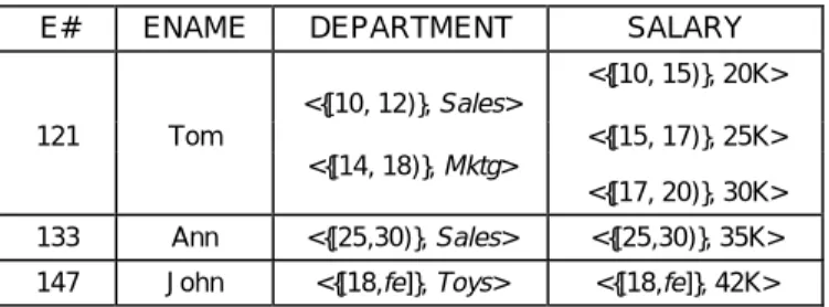
E# ENAME DEPARTMENT SALARY

<{[10, 12)}, Sales> <{[10, 15)}, 20K> 121 Tom <{[15, 17)}, 25K> <{[14, 18)}, Mktg> <{[17, 20)}, 30K> 133 Ann <{[25,30)}, Sales> <{[25,30)}, 35K> 147 John <{[18,fe]}, Toys> <{[18,fe]}, 42K> Fig. 3. EMP relation.

For requirement 7, any data model using temporal sets (elements) as timestamps naturally supports set-theoretic operations and set comparison tests on timestamps. How-ever, the case of time points and intervals is not straight-forward. Any data model using them should be able to simulate these operations.

3 T

T

R

D

M

In this section, we define a temporal relational data model. P(U) denotes the powerset of the set U, and ‘¥’ denotes Cartesian product operation.

DEFINITION 1. A temporal atom is an ordered pair <t, v> where t is a temporal set or an interval (t Õ T) and v is an atomic value (v Œ U).

The temporal atom <t, v> asserts that v is valid for the time period t, which may not be empty. If a is a temporal atom, then a.T and a.v denote its temporal set and value components, respectively. A temporal atom represents a historical value of an attribute. The history of an attribute of an object can be modeled by a set of temporal atoms.

There are four types of attributes in a temporal relation. If an attribute, say A, has atomic values, then its domain is a subset of U. If attribute A has temporal atoms, then DOM(A) Õ Uta where Uta = P(T) ¥ U. The domain of an at-tribute may also be a subset of P(U). In this case, the attrib-ute’s values are sets of atoms. Finally, an attribute may have sets of temporal atoms, in which case its domain is a subset of P(Uta).

DEFINITION 2. R(A₁, A₂, …, A_n) is a temporal relation scheme where n is its degree and A₁, …, A_n are its attributes. An attribute A_i has an associated domain, DOM(A_i).

R is an N1NF relation with a nesting depth of at most 1, i.e., its attributes can be sets of atoms or temporal atoms. In this study, we restrict nesting depth to 1 since it is capable of simulating all the other proposed temporal relational data models, excluding their feature we do not include in our discussion. Moreover, one level of nesting is sufficient to represent a history of objects and their relationships. However, in cases where a relationship is embedded into a relation as an attribute, more levels of nesting are needed, one level for the relationship and another level for the his-tory of the attribute that belongs to the relationship. It is also straightforward to generalize the conclusions of this study to arbitrarily nested temporal relations. In [13], we give the formal definition of a generalized relational data model that allows arbitrary levels of nesting.

DEFINITION 3. An instance of relation scheme R is a set of n-tuples, <a1, º, an >, where ai is the value of attribute Ai and n is its arity. Each ai is either an atom, a temporal atom, a set of atoms, or a set of temporal atoms.

We use the terms atom, temporal atom, set of atoms, and set of temporal atoms for the scheme and its instance. We also use the terms relation and temporal relation inter-changeably.

DEFINITION 4. A relational database schema D is {R, S, º} where R, S, º are relation schemes.

In Fig. 3, we show a heterogeneous employee relation, called EMP, over the scheme E# (employee number), ENAME (employee name), DEPARTMENT, and SALARY. E# and ENAME are atomic attributes, and DEPARTMENT and SALARY are attributes with temporal atoms. Note that there are no department values for Tom in the peri-ods [12, 4) and [18, 20). Perhaps he was not assigned to any department during this time. We can also convert E# and

ENAME into temporal atoms by assigning an appropriate validity period as their timestamps.

4 N

T

C

In this section, we define the Nested Tuple Calculus (NTC) language [13] for the temporal relational data model given in the previous section. We give the symbols and the well-formed formulae of the language, followed by their interpretations.

4.1 Symbols

• Predicate names: There is a finite number of predicate names, P, Q, R, S, … one for each relation instance in the database.

• Variables: There is a countable number of tuple vari-ables, s, t, u, v, … A variable has the same scheme and degree (arity) as the relation scheme it is associated with. Variables may be indexed. If s is a variable, then s[i] is an indexed variable where i is between 1 and the arity of s. s[i] can be an atom, a temporal atom, a set of atoms, or a set of temporal atoms. If s[i] is a temporal atom, s[i].v and s[i].T are also variables de-noting the value and the temporal set parts of this temporal atom, respectively. We use t as a special variable for time points and add a subscript whenever more time variables are needed. This is done for the sake of clarity; otherwise there is no need for such a distinction.

• Constants: There is a countable number of constant symbols, a, b, c, … Each constant has a scheme, an atom, a temporal atom, a set of atoms, or a set of tem-poral atoms.

4.2 Well-Formed Formulae

1) P(s); P is a predicate name and s is a variable.

2) s[i] op r[j]; s[i] op c; where op is one of =, ?, <, £, >, ≥; and s[i], r[j], and c are atoms. The position of oper-ands can be changed to form a new formula.

3) s[i].v op p[j].v; s[i].v op r[k]; or s[i].v op c; where op is one of =, ?, <, £, >, ≥; s[i] and p[j] are temporal atoms; and r[k] and c are atoms. The position of operands can be reflected to form a new formula.

4) s[i] = r[j]; r[j] = s[i]; s[i] = c; or c = s[i]; where s[i], r[j], and c have the same scheme, i.e., set of atoms, tempo-ral atom, or set of tempotempo-ral atoms. Here, = is an iden-tity test, and hence π may also be used. s[i].T = r[j].T is allowed if s[i] and r[j] are temporal atoms.

5) Formulae involving membership test:

• s[i] Œ r[j], where s[i] is an indexed variable that is an atom and r[j] is an indexed variable that is a set of atoms. If s[i] is a temporal atom, indexed vari-able r[j] is also a set of temporal atoms. In this for-mula, either of the indexed variables can be re-placed by an appropriate constant.

• s[i].v Œ r[j], where s[i] is a temporal atom and r[j] is a set of atoms. Either operand can be replaced by an appropriate constant.

• s[i] Œ r[j].T, where s[i] is an indexed variable that is an atom and r[j].T is also an indexed variable that is a temporal atom. Either of the indexed variables can be replaced by an appropriate constant. Fur-thermore, s[i].v can also be specified if s[i] is a temporal atom.

6) If y and l are formulae, so are y Ÿ l, y ⁄ l, and ÿy. 7) If y is a formula with the free variable s, then $sy(s)

and "sy(s) are formulae and s no longer occurs freely in y.

8) r[i] = {s(1)| y(s, u, v, …)} is a formula with free vari-ables s, u, v, … The variable s has arity 1 and does not occur freely in y. The scheme of indexed variable r[i] is a set of atoms or temporal atoms. In the resulting formula, variables u, v, … are free and s is bound. This formula is called a set constructor, and it may not be used in y.

4.3 Interpretation of Calculus Objects

The domain of interpretation for a calculus object x is fined relative to the set U, universe of atoms, and is de-noted by Domx(U). Atoms take their values from U. The

domain of interpretation for temporal atoms is Uta.

An interpretation of a constant c, denoted as I_c, is a member of Dom_c(U). If c is an atom or a set of atoms, then Dom_c(U) is U or P(U), respectively. If c is a temporal atom or a set of temporal atoms, then Dom_c(U) is Uta or P(Uta_), respectively. An interpretation of a predicate name P, de-noted as I_P, is a relation instance, and I_P Œ Dom_P(U). A vari-able s is interpreted as a tuple instance, and Is Œ Doms(U) where Doms(U) = L1 ¥ … ¥ Ln and n is the degree of s. For each i, Li is U, P(U), U

ta

, or P(Uta) if s[i] is an atom, set of atoms, temporal atom, or set of temporal atoms, respec-tively. Is(i) denotes the ith component of the tuple that is the interpretation of variable s. Formulae are interpreted as true or false by assigning interpretations to their constants, predicate symbols, and free variables.

The following are the rules for the interpretation of for-mulae in NTC.

1) P(s) is true if Is ΠIP.

2) s[i] op r[j] is true if Is(i) op Ir(j). s[i] op c is true if Is(i) op Ic.

3) s[i].v op p[j].v is true if Is(i).v op Ip(j).v. s[i].v op r[k] is true if Is(i).v op Ir(k). s[i].v op c is true if I_s(i).v op I_c. 4) s[i] = r[j] is true if I_s(i) = I_r(j). s[i] = c is true if I_s(i) = I_c. 5) s[i] Œ r[j] is true if I_s(i) Œ I_r(j). s[i].v Œ r[j] is true if Is(i).v Œ Ir(j). s[i] Œ r[j].T is true if Is(i) Œ Ir(j).T. 6) y Ÿ l is true if both y and l are true. y ⁄ l is true if either y or l is true. ÿy is true if y is false.

7) $sy(s) is true if there is at least one assignment to s which makes y(s) true, i.e., y(s) is true for at least one value of Is. "sy(s) is true if y(s) is true for any as-signment to s.

8) r[i] = {s(1)| y(s, u, v, º)} is satisfied (made true) by the interpretations Ir, Is, Iu, Iv, … of its free variables if the

following condition is met: Ir(i) equals the set of as-signments I_s satisfying y(s, u, v, ...) for the interpreta-tions I_u, I_v, º If there are no such tuples I_s, and I_r(i) is empty, then this formula evaluates to false. In other words, the set constructor formula does not create an empty set.

An NTC expression is {sk| y(s)} where s is a free variable with arity k and y(s) is a well-formed formula. An inter-pretation of this expression is the set of instances of s that satisfy the formula y(s), i.e., an element of Doms(U).

4.4 Safety of NTC

We define a safe subset of NTC according to the definition given in [24]. Let y be a formula with one free variable, t. The formula y is safe if it satisfies the following conditions:

1) The universal quantifier (") is not allowed. This is not a restriction, since the universal quantifier can always be replaced by the existential quantifier ($).

2) Whenever a ⁄ operator is used, the two subformulae connected, say y ⁄ l, should have the same free tuple variables.

3) Consider any maximal conjunct y1 Ÿ y2 Ÿ º Ÿ yn of y. All components of tuple variables appearing free in any y_i must be limited in the following sense:

a) If y_i is a nonnegated atomic formula in the form R(u), then all components of tuple variable u are limited.

b) If y_i is u[i] = c or c = u[i], where c is a constant, then u[i] is limited.

c) If yi is u[i] = v[j] or v[j] = u[i], and v[j] is limited, then u[i] is limited. Note that rules b and c apply to the parts of the temporal atoms as well. A tem-poral atom is limited if its temtem-poral set and value parts are both limited.

d) If yi is u[i] Πv[j] and v[j] is limited, then u[i] is limited. If u[i] is a temporal atom, its temporal set and value parts are also limited.

e) If yi is u[i] = {s,| y¢(s, u, v, …)} and y¢(s, u, v, …) is safe, then u[i] is limited.

4) A ÿ can apply only to a term in a conjunction of the type discussed in condition 3. Furthermore, there should be at least one nonnegated formula in a maximal conjunct.

We now give some examples, using the EMP relation of Fig. 3 to illustrate NTC. Answers to the example queries are shown in Fig. 4. For the reader’s convenience, we use at-tribute names instead of position indexes in the following NTC expressions.

QUERY 1. What are the names and salaries of those employ-ees in the Sales department at time 16?

{x(2)| ($r) (EMP(r) Ÿ ($u) ($z) (u Œ r[DEPARTMENT] Ÿ z Œ r[SALARY] Ÿ ($t) (t Œ u.T Ÿ t = 16 Ÿ t Œ z.T Ÿ u.v = ‘Sales’ Ÿ x[1] = r[ENAME] Ÿ x[2] = z.v)))}. QUERY 2. What are the histories of those employees who

have worked only in the Sales department?

{x(4)| ($r) (EMP(r) Ÿ

($u) (u Œ r[DEPARTMENT] Ÿ u.v = ‘Sales’ Ÿ ÿ($z) (z Œ r[DEPARTMENT] Ÿ

z.v ? ‘Sales’) Ÿ

x[1] = r[E#] Ÿ x[2] = r[ENAME] Ÿ x[3] = r[DEPARTMENT] Ÿ x[4] = r[SALARY]))}.

QUERY 3. What are the name and salary histories of the em-ployees whose current salary is the same as the salary of another employee when that employee was work-ing for the Sales department?

{x(2)| ($r)($s) (EMP(r) Ÿ EMP(s) Ÿ

($u) (u Œ r[SALARY] Ÿ now Œ r[SALARY].T Ÿ ($z)($y) (z Œ s[SALARY] Ÿ y Œ s[DEPARTMENT] Ÿ y.v = ‘Sales’ Ÿ ($t) (t Œ y.T Ÿ t Œ z.T Ÿ u.v = z.v) Ÿ x[1] = s[ENAME] Ÿ x[2] = s[SALARY])))}.

QUERY 4. What was the salary and department of Tom im-mediately after his last salary increase?

{x(3)| ($r) (EMP(r) Ÿ r[ENAME] = Tom Ÿ

($u)($s) (u Œ r[SALARY] Ÿ s Œ r[SALARY] Ÿ ($t1)($t2) (t2 < t1 Ÿ t1 Œ u.T Ÿ t2 Œ s.T Ÿ s.v < u.v Ÿ ÿ($z) (z Œ r[SALARY] Ÿ ($t₃) (t₃ Œ z.T Ÿ t₂ < t₃ Ÿ t₃ < t₁)) Ÿ ÿ($t4) (t1 < t4 Ÿ ($y)($w) (y Œ r[SALARY] Ÿ w Œ r[SALARY] Ÿ ($t5) (t5 < t4 Ÿ t4 Œ y.T Ÿ t5 Œ w.T Ÿ w.v < y.v Ÿ ÿ($q) (q Œ r[SALARY] Ÿ ($t6) (t6 Œ y.T Ÿ t5 < t6 Ÿ t6 < t4))) )) Ÿ ($h) (h Œ r[DEPARTMENT] Ÿ t1 Œ h.T Ÿ x[1] = r[ENAME] Ÿ x[2] = h.v Ÿ x[3] = u.v))))}.

We now give some useful propositions that will be needed in the remainder of the article.

ENAME SALARY

Tom 25K

Query 1

E# ENAME DEPARTMENT SALARY

133 Ann <{[25, 30)}, Sales> <{[25, 30)}, 35K> Query 2

∆ Query 3

ENAME DEPARTMENT SALARY

Tom Mktg 30K

Query 4 Fig. 4. Results of the example queries.

PROPOSITION 1. NTC can form the union, intersection, and dif-ference of temporal sets (and hence of temporal atoms). PROOF. Straightforward from the definition of NTC. † PROPOSITION 2. NTC can simulate formulae involving set

com-parison, e.g., set inclusion.

PROOF. Straightforward from the definition of NTC. † PROPOSITION 3. NTC can convert temporal atoms with temporal

sets to temporal atoms with intervals.

PROOF. Let R(A) be a relation scheme where values of at-tribute A are temporal atoms. We first take the Carte-sian product of the relation T with itself to obtain a relation (TI) having tuples giving all possible intervals over the temporal domain T. For each time interval in TI, we obtain the set of time points in this interval. Then, we select the time intervals containing time points in the temporal atoms of R. Some of these in-tervals are superset of inin-tervals in the temporal at-oms. Such intervals are weeded out to yield the final result. For the detailed proof, see [26]. † PROPOSITION 4. NTC can convert temporal atoms with temporal

sets to temporal atoms with time points.

PROOF. A conversion procedure similar to the one in the

proof of Proposition 3 can be devised. †

PROPOSITION 5. NTC can convert temporal atoms with intervals to equivalent temporal atoms with temporal sets.

PROOF. Combine the intervals of temporal atoms whose values are the same into a temporal set. It is obvious

that this can be done in NTC. †

5 A N

T

R

C

In traditional database theory, relational calculus (RC) is used as the standard in evaluating the expressive power of query languages [25]. A language that has the same expres-sive power as RC is called relationally complete. We use the same approach in defining temporal completeness as was used in [5], [6]. We take NTC as the yardstick against which a temporal language is evaluated. There are several reasons for this. First, NTC is a superset of relational calculus. Ad-ditionally, it has set membership test and set constructor formulae. If only 1NF relations are used, these formulae are not needed, and thus NTC reduces to the relational calcu-lus. Therefore, NTC subsumes the expressive power of re-lational calculus. Second, the data model of NTC is very powerful, and it meets all of the requirements listed in Sec-tion 2.1. It can handle both heterogeneous and homogene-ous tuples, since the latter is a subclass of the former. We believe that this model provides full representation of real-ity. Third, NTC can generate both relations in unique repre-sentation and weak relations, and allows conversion be-tween these two types of relations. Fourth, there is a tempo-ral relational algebra that has the same expressive power as NTC [13]. Fifth, NTC provides conversion in both direc-tions, between various temporal data models and our tem-poral relations.

In the following, we compare various temporal query

languages with NTC. In these comparisons, we consider only those features of the temporal query languages rele-vant to the requirements specified in Section 2.1. Some of these languages may have additional features that we briefly mention but do not consider in our comparisons. We provide a transformation procedure from the temporal re-lational data model to each of the proposed data models. The reverse, conversion from these models to temporal re-lations, can similarly be done by NTC. The only exception is HRDM [8]; for an explanation see the last paragraph in Section 2. After the transformation procedure, we give an equivalent NTC expression for the language constructs of these models, showing that NTC is as expressive as these languages and that these languages are bounded in expres-sive power by NTC.

In the remainder of the article, we will write NTC for-mulae as if all the attributes of a temporal relation consist of sets of temporal atoms. We assume that attributes whose values are atoms or sets of atoms (i.e., E# and ENAME) are assigned appropriate timestamps. We will also use at-tribute names instead of position indexes, whenever it is more convenient.

6 G

’

A

Gadia proposes a homogeneous relational model [9]. Each attribute value is assigned a temporal element. A temporal assignment to an attribute A_i is a function from a temporal element into the domain of A_i. Each tuple has a temporal domain that varies from tuple to tuple. However, all attrib-utes of a tuple must have the same temporal domain. In other words, temporal tuples in his model are homogene-ous. A subset of attributes of R is defined as the temporal key for r, a (temporal) relation over scheme R, if that subset is a key for all snapshots of r. Fig. 5 illustrates the EMP relation under Gadia’s model. Gadia introduces a relational algebra and a temporal tuple relational calculus for this model. He then proves the equivalence of the algebra and the calculus. In the next subsection, we will consider only his calculus, which we call GTC.

PROPOSITION 6. Gadia’s relations can be generated from a tempo-ral relation by NTC.

PROOF. Directly follows from the equality of temporal sets

and temporal elements. †

6.1 Expressiveness of GTC and NTC

1) Relation formula. Let R be a predicate name and x be a tuple variable in GTC. R(x) is also a formula in NTC. 2) Q-comparison. Let Q be a binary comparator, A and B

be two attributes that are Q-comparable, and c be a constant in the domain of attribute A. Also let x and y be tuple variables. Then,

• x(A) Q y(B) ∫

($u)($z) (u Œ x[A] Ÿ z Œ y[B] Ÿ

($t) (t Πu.T ٠t Πz.T ٠u.v Q z.v ٠d)).

• x(A) Q c ∫

d represents an NTC expression to restrict the time of x(A) and y(B) if they appear in the target specifi-cation. It is null otherwise. d is the same as the se-lection formula without a Boolean condition of Bhargava and Gadia (see Section 7, case 3).

3) ' x l(x) is a temporal expression in GTC where l(x) is a formula with the free variable x. ' x l(x) represents the temporal domain of the tuple denoted by x. It can be computed by taking the union of temporal sets of all temporal atoms in any attribute A of tuple x. Let y(x) be the NTC expression for l(x).

' x l(x) ∫ ($x)($u) (u Œ x[A] Ÿ t Œ u.T Ÿ y(x)). Note that t may be existentially quantified, depending on the use of ' x l(x) in the larger GTC expression. 4) Let v₁ and v₂ be two temporal expressions in

GTC, and let l1(t1) and l2(t2) be the corresponding

NTC expressions.

• v1 , ∫ ($t1) (l1(t1) Ÿ t ? t1) Ÿ t Œ T,

• v1 < v2 ∫ ($t1)($t2) (l1(t1) Ÿ l2(t2) Ÿ (t = t1 ⁄ t = t2)), • v1 > v2 ∫ ($t1)($t2) (l1(t1) Ÿ l2(t2) Ÿ t = t1 Ÿ t = t2), • v1 - v2 ∫ ($t1)($t2) (l1(t1) Ÿ l2(t2) Ÿ t = t1 Ÿ t ? t2).

5) For a temporal expression v and a tuple variable x, x : v is a formula in GTC such that x : v restricts the temporal domain of the tuple x to 'x > v. Let the scheme of x be A1, …, An. The equivalent formula in NTC is:

x : v ∫

($t)($u1) … ($un)

(t Œ u1.T Ÿ … Ÿ t Œ un.T Ÿ l(t) Ÿ u1 Œ x[A1] Ÿ … Ÿ un Œ x[An]) where l(t) is an NTC expression for v. If the GTC expression returns any attributes, then the temporal domain of these attributes should also be restricted to 'x > v. In this case, the GTC expression is the same as case 3 in Section 7 where there is no Boolean formula.

Logical operators, quantification, and constant temporal elements of GTC can directly be expressed in NTC.

{x,| l(x)} is a relational expression in GTC where l(x) is a formula with one free variable. The corre-sponding temporal relational calculus expression in NTC is given as {x(n)|y(x)} where y(x) ∫ l(x), n is the degree of the result.

PROPOSITION 7. NTC is at least as expressive as GTC.

PROOF. Directly follows from the preceding analysis. † GTC meets only requirements 1 and 5 listed in Section 2.1. However, it cannot convert weak relations into relations in unique representation. GTC does not satisfy requirement 2, since it cannot express query 3 in Section 4. It cannot handle multivalued attributes, since attribute values are defined as functions of time. Moreover, GTC does not have the re-grouping capability.

7 B

G

’

A

Bhargava and Gadia introduce a temporal relational data model that includes a data history store and a transaction log as parts of their zero information loss model for database transactions [12]. We consider only the data history store, since transaction data is beyond the scope of this study. A data history relation is the same as the homogeneous tempo-ral relation of Gadia [9]. Fig. 5 shows the EMP relation in the data store model. Bhargava and Gadia introduce an algebra for their data model. We will call this algebra BGA and compare it with NTC. An equivalent tuple calculus language is given in [7].

7.1 Expressiveness of BGA and NTC

In order to demonstrate that NTC is at least as powerful as BGA in expressiveness, we will consider all algebraic ex-pressions of BGA and give their semantic equivalents in NTC. We first examine the binary comparators, which play a crucial role in the algebraic expressions of BGA. Given two Q-comparable attributes A and B, and a constant c, then A Q B, A Q c, and c Q A are valid formulae used in selection operations of BGA. Equivalent NTC expressions are the same as the ones provided for Q-comparison in Section 6.1.

Bhargava and Gadia classify algebraic expressions into temporal expressions, Boolean expressions, and relational expres-sions. We will define expressions in each category and then show that they are expressible by NTC formulae.

1) Temporal expressions. Basic temporal expressions in BGA are of the form [[A]], [[r]], [[A Q B]], and [[A Q c]]. The notation [[…]] represents the temporal domain of the object specified. More complex expres-sions can be formed by using the union (<), intersec-tion (>), and difference (-) operaintersec-tions. Note that in-corporating the converted subformula into the larger NTC expression may sometimes require quantifica-tion over the free variables. Let x be a tuple variable.

E# ENAME DEPARTMENT SALARY

[10, 12) [10, 12) [10, 12) [10, 12) Sales < 20K < 121 < Tom [14, 15) [14, 18) [14, 18) [14, 18) Mktg [15, 17) 25K [17, 18) 30K [25, 30) 133 [25, 30) Ann [25, 30) Sales [25, 30) 35K [18, fe] 147 [18, fe] John [18, fe] Toys [18, fe] 42K Fig. 5. The temporal relation EMP in Gadia’s temporal model.

• Temporal elements are also temporal expressions. The NTC equivalent of a constant temporal ele-ment n, [l₁, u₁) < … < [l_n, u_n), is:

(t ≥ l1 Ÿ t < u1) ⁄ … ⁄ (t ≥ ln Ÿ t < un) Ÿ t Œ T, • [[A]] ∫ ($u) (t Œ u.T Ÿ u Œ x[A]),

• [[A Q B]] ∫ ($u)($z) (t Œ u.T Ÿ t Œ z.T Ÿ u.v Q z.v Ÿ u Œ x[A] Ÿ z Œ x[B]),

• [[A Q c]] ∫ ($u) (t Œ u.T Ÿ u.v Q c Ÿ u Œ x[A]),

• [[r]] ∫ ($x)($u) (P(x) Ÿ t Œ u.T Ÿ u Œ x[A]) where A is an attribute of R and P is an NTC predicate name representing r.

2) Boolean expressions. TRUE, FALSE, A Q B, and m Õ n, where m and n are temporal expressions, are the ba-sic Boolean expressions in BGA. More complex Boolean expressions can be obtained by using the logical connective Ÿ and ⁄ and the negation ÿ. TRUE and FALSE can easily be represented in NTC. The Boolean expressions of the form A Q B are expressi-ble in NTC as shown under Q-comparison in Section 6.1. Logical connectives of BGA directly correspond to the logical connectives of NTC. As for the expres-sion m Õ n, it is expressible in NTC (Proposition 2). 3) Relational expressions. Restructuring operator, union,

selection, difference, projection, Cartesian product, and renaming are all expressible in NTC. We illustrate the selection operation below. Semantic equivalents of other expressions in NTC can be found in [26].

Selection (s). Given a relational expression r, a Boolean expression y, and a temporal expression m, the selection operation s(r ≠ m, y) of BGA selects those tuples of r satisfying the expression y and re-stricts their temporal domain to m. Let P, f(t), and y¢ be the NTC expressions for r, m, and y, respectively. We first determine the tuples satisfying y¢ and then restrict the temporal domain of these tuples to f(t). Each attribute of P is restricted by m individually, which afterwards combines by forming a side-by-side copy of P to regain the original structure. In the following, for two tuple variables x and y we use x = y as a shorthand for x[A₁] = y[A₁] Ÿ … Ÿ x[A_n] = y[A_n].

l1(x) ∫ P(x) Ÿ ($y) (P(y) Ÿ x = y Ÿ y¢)

where y¢ is a formula on tuple variable y, l₂(x) ∫

($y) (l1(y) Ÿ x[A1] = y[A1] Ÿ … Ÿ x[An] = y[An] Ÿ x[An+1] = y[A1] Ÿ … Ÿ x[An+n] = y[An]),

λA1(x) ∫

($y) (l2(y) Ÿ x[A1] = y[A1] Ÿ … Ÿ x[An] = y[An] Ÿ ($z) (z Œ y[An+1] Ÿ x[An+1].v = z.v Ÿ ($u) (x[An+1].T = u Ÿ u = {t | f(t) Ÿ t Œ n+1].T Ÿ t Œ z.T}))), ′ λA1(x) ∫ ($y) (l_A1(y) Ÿ

x[A1] = y[A1] Ÿ … Ÿ x[An] = y[An] Ÿ

x[An+1] = {z[An+1] | λA1(z) Ÿ z[A₁] = y[A₁] Ÿ … Ÿ z[A_n] = y[A_n]}). The last two steps should be repeated for the remaining attributes Ai, i.e., λAi and λ′Ai for 2 £ i £ n, by changing

z Œ y[An+1] to z Œ y[An+i] in λA1(x). Finally,

l(x) ∫ ($y₁) … ($y_n) (λ′_A 1(y1) Ÿ … Ÿ λ′An(yn) Ÿ y1 = y2 Ÿ y2 = y3 Ÿ … Ÿ yn-1 = yn Ÿ x[A₁] = y₁[A_n+1] Ÿ … Ÿ x[A_n] = y_n[A_n+1]). l(x) is the desired equivalent expression for s(r ≠ m, y). PROPOSITION 8. NTC is at least as expressive as BGA.

PROOF. Direct result of the previous conversions. † BGA meets requirements 1, 2, 5, 6, and 7 of Section 2.1. BGA retrieves relations in unique representation from one relation. It may return weak relations when tuple compo-nents from several relations appear in the target specifica-tion. The result can be converted to unique representation by the restructuring operation.

8 C

C

’

A

Clifford and Croker introduce a temporal relational data model, namely HRDM, and an algebra based on the notion of lifespans [8]. A subset, L, of T is called a lifespan. They attach time to every tuple and every attribute. Each tuple is associated with a lifespan and can have values only at time points in its lifespan. Each attribute of a relation scheme R, including its key attributes, is assigned a value domain, which is a set of atomic values, and a lifespan. Attribute values are timestamped by time points and seen as func-tions from time to the values in the value domain. All the key attributes must be constant-valued. Fig. 6 illustrates the employee relation EMP in this model. LTuple denotes the lifespan for each tuple. Note that the discontinuity in de-partment values of Tom’s tuple requires the introduction of a special null value. Clifford and Croker define a historical algebra, which we will call CCA. In order to show that NTC is at least as expressive as CCA, we provided an equivalent expression in NTC for each algebraic operation and expres-sion in CCA [26].

PROPOSITION 9. NTC can generate an equivalent historical rela-tion in HRDM from a temporal relarela-tion.

PROOF. See [26] for the proof. †

CCA meets requirement 1 and partially meets require-ment 5 of Section 2.1. It retrieves relations in unique repsentation as well as weak relations. CCA does not meet re-quirement 2, since it cannot express query 3 in Section 4. It does not support multivalued attributes, since attribute values are defined as functions of time. CCA does not have the capability to convert weak relations to unique relations and to regroup temporal data.

9 T

L

L

In [15], Clifford, Croker, and Tuzhilin (CCT) name the N1NF temporal relational models as temporally grouped and the 1NF temporal relational models as temporally ungrouped models. We now examine their grouped model and con-sider the expressive power of its associated language, Lh.

In the temporally grouped model, as in HRDM, every tuple has a lifespan, and its attributes can have values at the time points in its lifespan. Each attribute value is a temporal-based function that assigns a value from its asso-ciated domain to time points in tuple’s lifespan. Tuples of the temporally grouped model are homogeneous.

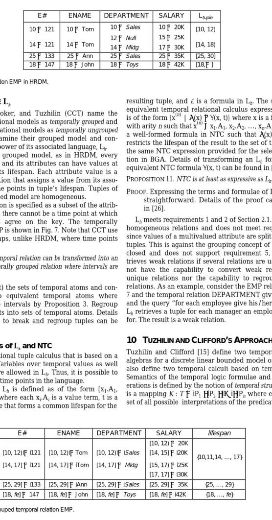
The key of a relation is specified as a subset of the attrib-utes A of R such that there cannot be a time point at which two different tuples agree on the key. The temporally grouped relation EMP is shown in Fig. 7. Note that CCT use intervals as timestamps, unlike HRDM, where time points are the timestamps.

PROPOSITION 10. A temporal relation can be transformed into an equivalent temporally grouped relation where intervals are the timestamps.

PROOF. Break (unnest) the sets of temporal atoms and con-vert them into equivalent temporal atoms where timestamps are intervals by Proposition 3. Regroup (nest) the results into sets of temporal atoms. Details of a procedure to break and regroup tuples can be found in [13].

9.1 Expressiveness of Lh and NTC

Lh is a temporal relational tuple calculus that is based on a many-sorted logic. Variables over temporal values as well as ordinary values are allowed in Lh. Thus, it is possible to explicitly refer to the time points in the language.

An expression in Lh is defined as of the form [x1.A1,

x2.A2, …, xn.An : t]f where each xi.Ai is a value term, t is a free temporal variable that forms a common lifespan for the

resulting tuple, and f is a formula in L_h. The semantically equivalent temporal relational calculus expression in NTC is of the form {x(n) | y(x) Ÿ l(x, t)} where x is a free variable with arity n such that x(n) ∫ x₁.A₁, x₂.A₂, …, x_n.A_n and y(x) is a well-formed formula in NTC such that y(x) ∫ f. l(x, t) restricts the lifespan of the result to the set of t values. It is the same NTC expression provided for the selection opera-tion in BGA. Details of transforming an Lh formula to an equivalent NTC formula l(x, t) can be found in [26]. PROPOSITION 11. NTC is at least as expressive as Lh.

PROOF. Expressing the terms and formulae of Lh in NTC is straightforward. Details of the proof can be found in [26].

Lh meets requirements 1 and 2 of Section 2.1. Lh supports homogeneous relations and does not meet requirement 4, since values of a multivalued attribute are split into several tuples. This is against the grouping concept of Lh. Lh is not closed and does not support requirement 5, since it re-trieves weak relations if several relations are used. Lh does not have the capability to convert weak relations into unique relations nor the capability to regroup temporal relations. As an example, consider the EMP relation in Fig. 7 and the temporal relation DEPARTMENT given in Fig. 2a and the query “for each employee give his/her managers.” L_h retrieves a tuple for each manager an employee worked for. The result is a weak relation.

10 T

C

’

A

Tuzhilin and Clifford [15] define two temporal relational algebras for a discrete linear bounded model of time. They also define two temporal calculi based on temporal logic. Semantics of the temporal logic formulae and algebra op-erations is defined by the notion of temporal structure, which is a mapping K : T Æ P1 ¥ P2 ¥ º ¥ Pn where each Pi is the set of all possible interpretations of the predicate Pi. Hence,

E# ENAME DEPARTMENT SALARY L_tuple

10 Æ 121 10 Æ Tom 10 ÆSales 10 Æ 20K [10, 12) 12 ÆNull 15 Æ 25K 14 Æ 121 14 Æ Tom 14 ÆMktg 17 Æ 30K [14, 18) 25 Æ 133 25 Æ Ann ₂₅ ÆSales 25 Æ 35K [25, 30] 18 Æ 147 18 Æ John ₁₈ ÆToys 18 Æ 42K [18,Æ] Fig. 6. The temporal relation EMP in HRDM.

E# ENAME DEPARTMENT SALARY lifespan

[10, 12) Æ 20K [10, 12) Æ 121 [10, 12) ÆTom [10, 12) Æ Sales [14, 15] Æ 20K {10,11,14, …, 17} [14, 17] Æ 121 [14, 17] Æ Tom [14, 17] Æ Mktg [15, 17) Æ 25K [17, 17] Æ 30K [25, 29] Æ 133 [25, 29] Æ Ann [25, 29] Æ Sales [25, 29] Æ 35K {25, …, 29} [18, fe] Æ 147 [18, fe] Æ John [18, fe] ÆToys [18, fe] Æ 42K {18, …, fe} Fig. 7. The temporally grouped temporal relation EMP.

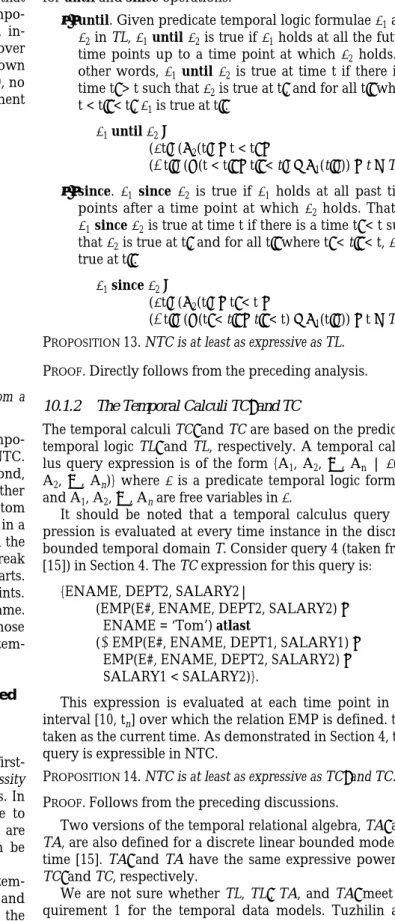
K assigns to each time point an instance of each of the predicates P₁, P₂, º, P_n at that time point. This means that each predicate P_i in a temporal structure provides a tempo-ral relation and that each relation changes over time, in-stead of each of its individual attributes changing over time. The temporal structure for the EMP relation is shown in Fig. 8. Note that for the time points 12, 13, 18, and 19, no data is specified for Tom since there are no department values.

Time Ki (EMP)

i = 10, 11 EMP(121, Tom, Sales, 20K)

i = 14 EMP(121, Tom, Mktg, 20K)

i = 15, 16 EMP(121, Tom, Mktg, 25K)

i = 17 EMP(121, Tom, Mktg, 30K)

i = 18 … 24 EMP(147, John, Toys, 42K)

i = 25 … 29 EMP(133, Ann, Sales, 35K) EMP(147, John, Toys, 42K)

i = 30 … fe EMP(147, John, Toys, 42K) Fig. 8. The temporal structure for the EMP relation.

PROPOSITION 12. A temporal structure can be obtained from a temporal relation.

PROOF. We give a sketch of a procedure to obtain a tempo-ral structure from a tempotempo-ral relation by using NTC. First, break (unnest) sets of temporal atoms. Second, trim the temporal set of each attribute by every other attribute. This makes sure that every temporal atom has the same temporal set, i.e., there is no change in a tuple for this period. Third, discard the time of all the attributes except one attribute, say, A1. Then break

attribute A1 into its temporal set and value parts.

Fourth, break this temporal set into its time points. Then group (nest) the tuples whose time is the same. Finally, group the time points of the tuples whose value parts are the same. This gives the desired tem-poral structure.

10.1 Expressiveness of the Temporal Calculi Based on Temporal Logics

10.1.1 Temporal Logic TL¢

TL¢ is a predicate temporal logic derived from the first-order logic by associating the temporal operators necessity (u), possibility (e), and next (o), and their past versions. In this logic, time is not explicitly referenced. Reference to time is embedded in the temporal operators and there are no temporal constants or temporal variables. TL¢ can be expressed by NTC [26].

Another type of temporal logic, TL, uses the binary tem-poral operator until and its past version since. Tuzhilin and Clifford show that TL is more powerful than TL¢ for the discrete linear bounded model of time (cf. Proposition 1 in [15, p. 15]). Other temporal operators such as atfirst and its past version atlast are allowed in TL as well. These opera-tors can be expressed in terms of the until and since

op-erators and vice versa. Below we give the NTC expressions for until and since operations.

• until. Given predicate temporal logic formulae f₁ and f₂ in TL, f₁ until f₂ is true if f₁ holds at all the future time points up to a time point at which f₂ holds. In other words, f₁ until f₂ is true at time t if there is a time t¢ > t such that f₂ is true at t¢, and for all t¢¢ where t < t¢¢ < t¢, f1 is true at t¢¢.

f₁ until f₂ ∫

($t¢) (y2(t¢) Ÿ t < t¢ Ÿ

("t¢¢) (ÿ(t < t¢¢ Ÿ t¢¢ < t¢) ⁄ y1(t¢¢))) Ÿ t Œ T. • since. f1 since f2 is true if f1 holds at all past time

points after a time point at which f2 holds. That is, f₁ since f2 is true at time t if there is a time t¢ < t such

that f2 is true at t¢, and for all t¢¢ where t¢ < t¢¢ < t, f1 is

true at t¢¢. f₁ since f2 ∫

($t¢) (y2(t¢) Ÿ t¢ < t Ÿ

("t¢¢) (ÿ(t¢ < t¢¢ Ÿ t¢¢ < t) ⁄ y1(t¢¢))) Ÿ t Œ T.

PROPOSITION 13. NTC is at least as expressive as TL.

PROOF. Directly follows from the preceding analysis. †

10.1.2 The Temporal Calculi TC¢ and TC

The temporal calculi TC¢ and TC are based on the predicate temporal logic TL¢ and TL, respectively. A temporal calcu-lus query expression is of the form {A₁, A₂, º, A_n | f(A_i, A₂, º, A_n)} where f is a predicate temporal logic formula and A₁, A₂, º, A_n are free variables in f.

It should be noted that a temporal calculus query ex-pression is evaluated at every time instance in the discrete bounded temporal domain T. Consider query 4 (taken from [15]) in Section 4. The TC expression for this query is:

{ENAME, DEPT2, SALARY2|

(EMP(E#, ENAME, DEPT2, SALARY2) Ÿ

ENAME = ‘Tom’) atlast

((EMP(E#, ENAME, DEPT1, SALARY1) Ÿ

EMP(E#, ENAME, DEPT2, SALARY2) Ÿ

SALARY1 < SALARY2)}.

This expression is evaluated at each time point in the interval [10, tn] over which the relation EMP is defined. tn is taken as the current time. As demonstrated in Section 4, this query is expressible in NTC.

PROPOSITION 14. NTC is at least as expressive as TC¢ and TC. PROOF. Follows from the preceding discussions. †

Two versions of the temporal relational algebra, TA¢ and TA, are also defined for a discrete linear bounded model of time [15]. TA¢ and TA have the same expressive power as TC¢ and TC, respectively.

We are not sure whether TL, TL¢, TA, and TA¢ meet re-quirement 1 for the temporal data models. Tuzhilin and Clifford, in [15], do not provide a complete definition for these languages. It is not clear whether time can explicitly be referenced in a selection formula. Moreover, a temporal structure is, by definition, homogeneous, and it is possible

to compare two database instances at different time points only if all of the required relations are defined at these points. These languages support multivalued attributes. It is claimed that these languages return the same type of ob-jects as the type of their operands [15]. Definitions of their operations do not provide sufficient detail to determine the validity of this claim.

11 S

’

A

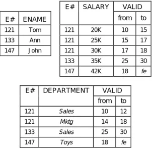
Snodgrass adds implicit timestamps for valid time and transaction time to 1NF relations [10]. We consider only valid time in the following analysis. There are two types of temporal relations:

• interval relations and • event relations.

In an interval relation, there exist two temporal attributes for each tuple. These two additional attributes, valid-from and valid-to, determine the time interval during which the tuple is valid. For an event relation, there is only one tem-poral attribute, named valid-at. In this way, the validity of each tuple is defined for a single point in time. By defini-tion, the tuples of the relations in this model are homoge-neous. Fig. 9 shows the EMP relation for Snodgrass’s tem-poral relational data model.

E# SALARY VALID E# ENAME from to 121 Tom 121 20K 10 15 133 Ann 121 25K 15 17 147 John 121 30K 17 18 133 35K 25 30 147 42K 18 fe E# DEPARTMENT VALID from to 121 Sales 10 12 121 Mktg 14 18 133 Sales 25 30 147 Toys 18 fe

Fig. 9. The EMP relation in the Snodgrass model.

PROPOSITION 15. In NTC, a nested temporal relation can be con-verted into equivalent 1NF relations in the Snodgrass model. PROOF. First, project the key attribute(s) (E# in EMP

rela-tion) and each of the temporal attributes into a sepa-rate relation. Secondly, break (unnest) the temporal attribute(s) in each relation into temporal atoms. Then, break the temporal atoms into their intervals by Proposition 3. Finally, place the end points of an in-terval in a tuple as the valid-from and valid-to attrib-utes. Note that this process is reversible. †

11.1 Expressiveness of TQuel and NTC

Snodgrass develops a temporal query language, TQuel, by augmenting Quel statements with new clauses, namely When, Valid, and “As of.” The “As of” clause, which rolls back the database to a previous time point is beyond the scope of this study. The When clause performs temporal selection. As for the Valid clause, it determines the valid interval (point) of the tuples derived as the result of the query. The Quel retrieve statement has the form:

range of r1 is R1 … range of rq is Rn retrieve r_i A_j r_i A_j s s 1⋅ 1 ⋅

F

H

I

K

In this expression, w is a Boolean formula, and t is an expression made up of temporal predicates. v1 and v2 are

temporal expressions specifying the end points of an inter-val over which the resulting tuple is inter-valid. t can be trans-lated into NTC in a straightforward manner by specifying the value components of temporal atoms. The temporal expression w includes predicates like overlap and extend, which can be done by set operations in NTC. The predicates begin of and end of refer to the end points of intervals. Since NTC uses temporal sets, the end points of intervals in a temporal set can be obtained by Proposition 3. The interval specified in the Valid clause is used to restrict the time of the result. This can be implemented in NTC as explained for the selection operation of BGA (Section 7.1).

As an alternative, Snodgrass shows in [10] that each TQuel statement has an equivalent expression in tuple cal-culus. This equivalent expression of tuple calculus is also a valid NTC expression, since NTC subsumes tuple calculus. PROPOSITION 16. NTC is at least as expressive as TQuel.

PROOF. Convert the nested temporal relations to equivalent relations in the Snodgrass model. Apply the equiva-lent tuple calculus expression for the TQuel query. Reform a nested temporal relation from the result by

Proposition 5. †

TQuel meets requirements 1, 2, 4, and 5 of temporal data models (see Section 2.1). However, it cannot compare an attribute whose values are temporal with the tuple time-stamps. This prevents TQuel from satisfying requirement 1 completely. TQuel requires that tuples be collapsed, if pos-sible, in the result. But this requirement is not built into the logic of equivalent tuple calculus expressions. TQuel does not have a regrouping capability.

12 L

J

’

A

The data model of Lorentzos and Johnson ([16], [2, chapter 3]) is basically similar to the data model of Snodgrass. A rela-tion can have three addirela-tional attributes, Fdate, Tdate, and/or Date. The first two attributes specify the interval during which a tuple is valid, whereas Date specifies the time point at which a tuple is valid. The model allows

switching between interval and point representations. It also supports more than one timestamp, which we do not discuss here since it is beyond the scope of our study. Proposition 15 allows conversion of a nested temporal rela-tion into equivalent relarela-tions in Lorentzos and Johnson’s model. Lorentzos and Johnson propose an algebra that we will call LJA. A few new operations are defined in LJA; we examine them below.

1) FOLD. This operation converts a relation in which data is timestamped with time points to an equivalent relation in which the data is timestamped with time intervals. In terms of algebraic operations, grouping (nesting) the time points of tuples whose value parts are the same yields a relation where each tuple has a set of time points representing an interval. The end points of each interval can be extracted in a way similar to the proof of Proposition 3 and then placed as the Fdate and Tdate attributes.

2) UNFOLD. The UNFOLD operation converts a relation in which data is stamped with time intervals to an equivalent relation in which data is stamped with time points. This can also be done by NTC expres-sions in a straightforward way.

3) EXTEND. This operation extracts the time points of intervals in a folded relation. That is, the time inter-vals are maintained, but for each time point in an in-terval of a tuple, the tuple is repeated. The EXTEND operation can be done in a manner similar to the UNFOLD operation except that the Fdate and Tdate attributes are kept for each tuple obtained in this way. PROPOSITION 17. NTC is at least as expressive as LJA.

PROOF. Direct consequence of the preceding analysis. † LJA meets requirements 1, 2, 4, 5, and 6 of Section 2.1. LJA’s relations are homogeneous; however, nonhomogene-ous tuples can be created in a Cartesian product operation. Overlapping or adjacent intervals can be restructured into one single interval. LJA does not have full support for set-theoretic operations.

13 O

A

In this section, we briefly discuss other data models and their languages.

Navathe and Ahmed [17] use tuple timestamping and 1NF relations that are the same as in Fig. 9, extend SQL for temporal data manipulation, and propose an algebra that we call NAA. NAA meets requirements 1, 2 and 4, and partially meets 5.

Sarda [18] also uses a temporal data model based on 1NF relations. He proposes a temporal extension to SQL and defines a relational algebra that we call SA. This algebra includes Expand and Coalesce operations in addition to regular relational algebra operations. The Expand and Coa-lesce operations are similar to the FOLD and UNFOLD op-erations of LJA, which can be expressed in NTC. Its concur-rent Cartesian product operation is similar to the ones in other homogeneous data models. SA meets requirements 1, 2, and 4, and partially meets 5.

McKenzie and Snodgrass [19] propose a 1NF relational model where attribute values are timestamped by temporal sets. Each attribute value is a temporal atom. They also de-fine an algebra, which we call MSA. Set-theoretic opera-tions of MSA can be expressed in NTC in a manner similar to the set operations of BGA. In these operations, the equality of key attributes is replaced by the equality of all the attribute values. Translation of Cartesian product and selection operations into NTC expressions is straightfor-ward. The temporal derivation operation performs a tem-poral selection operation and restricts the time of qualifying tuples. This operation can be expressed in a manner similar to the selection operation of BGA. MSA meets requirements 1, 2, 3, and 4, and partially meets 5.

Tansel uses intervals to timestamp attribute values in N1NF relations (Clifford and Tansel in [20] and Tansel in [21]). Here, a temporal atom is called a triplet. This model is also used in [5] by adding lifespans to tuples. The EMP re-lation of Fig. 7 is an example for this model when tuple lifespans are dropped. Tansel defines an algebra (TaA) that includes restructuring and temporal operators in addition to regular algebra operations. Operations are defined at the attribute level. This algebra meets all of the requirements listed in Section 2.1. NTC is more expressive than this algebra since it can form a powerset of a relation, whereas this algebra cannot. This algebra is generalized to arbitrar-ily nested relations and augmented with a looping con-struct to have the same expressive power as NTC [13], [27]. HQUEL [22] and Time-by-Example [28] are two user-friendly query languages based on a tuple calculus equiva-lent to this algebra.

14 S

C

We have identified requirements for temporal databases and have analyzed temporal query languages with respect to these requirements. We have also defined a calculus lan-guage, NTC, that meets all of these requirements. We have compared the expressive power of proposed temporal query languages to that of NTC and have shown that NTC is as expressive as these languages and subsumes their ex-pressive power.

Table 1 is a comparative summary of the temporal query languages with respect to the requirements identified in Section 2.1. All the languages meet requirement 1, i.e., that the model be able to query a database state at a time point, except TL, TL¢, TC, and TC¢, which do not seem to support explicit reference to time. GTC, BGA, and L_h do not seem to be able to access any arbitrary value in the history of an attribute [7]. Most of the temporal languages except GTC and CCA support querying two different database states simultaneously (requirement 2). LJA, MSA, NTC, and TaA support nonhomogeneous relations (requirement 3). The rest are all based on homogeneous relations in both attrib-ute and tuple timestamping. BGA, CCA, and GTC do not support multivalued attributes (requirement 4), because they see attribute values as functions from time to values. All languages based on 1NF relations support multivalued attributes, albeit with data redundancy, since they split the data into several tuples. This is also the case for the