Selçuk J. Appl. Math. Selçuk Journal of Vol. 5. No.2. pp. 15-24, 2004 Applied Mathematics
An Approximate Solution of Burgers Equation by Di¤erential Trans-form Method
Fatma Ayaz1 and Galip Oturanç2
1Department of Mathematics, Gazi University, Ankara 06500,Turkey;
e-mail:fayaz@ gazi.edu.tr
2Research Center of Applied Mathematics, Selcuk University, Konya, Turkey
e-mail:goturanc@ selcuk.edu.tr
Received : September 9, 2004
Summary.In this paper, we investigate some applications of di¤erential trans-form method for solving the linear and nonlinear partial di¤erential equations with appropriate initial and boundary conditions. In order to test and compar-ison of the approximate solutions obtained from di¤erential transform method where we have studied two test problems. In the …rst problem, a closed form solution of the heat equation, which can be obtained from Bu{rgers’ equation by omitting the nonlinear term in it, have been found easily. In the second problem, an approximate solution to the Burgers’ equation under appropriate conditions has been found for only the small values of t (time variable) and vis-cosity, . For decreasing visvis-cosity, which is di¢ cult task in the solution, it has seen that no signi…cant di¤erence in the solution for 0 < t < 0:005: The results have showed that the method can easily be applied both linear and nonlinear partial di¤erential equations.
Key words: Burgers equation; Heat equation; Di¤erential transform method.
1. Introduction
In this paper, we consider the Burgers’equation
(1) ut+ " u ux= uxx;
where "and , which is the kinematics viscosity, are parameters and the sub-scripts t and x denote di¤erentiation. The wide varieties of physically signi…cant problems can be modeled by nonlinear partial di¤erential equations. Burgers
equation is one of the very important equations in order to model turbulence [1] and the approximate theory of ‡ow through a shock wave traveling in a viscous ‡uid [2]. There are also a few number nonlinear partial di¤erential equations in the literature which can be solved exactly for a restricted set of initial data and the Burgers’equation is one of them. However, di¢ culties appear in the solution of Burgers’equation for small values of viscosity. The Analytical studies related to the Burgers’equation were surveyed in [3]. A variety of numerical techniques had also been used to solve Burgers equations which were cited in [4,5]. Both analytical and numerical methods have disadvantages as well as advantages but our aim is not to discuss these but consider a new series method.
In this study, the di¤erential transform method has been used to solve heat equation and one-dimensional Burgers’ equation for the small values of t and : A scheme of the present paper is as follows: Section 2 deals with de…nitions and operations of two-dimensional di¤erential transform method. In section 3, two test problems are considered to solve by the present method and the last section contains the review of the results and discussion
2. De…nition and operations of the two-dimensional di¤erential trans-form
Di¤erential Transform method was …rst considered by G.E. Pukhov [6] who solved linear and nonlinear initial value problems in electric circuit analysis. The technique is an iterative procedure for obtaining Taylor series coe¢ cients for the solution of ordinary or partial di¤erential equations. An advantage of the method is simplicity of its practical application and can be applicable to many problems. When the technique is compared with the classical techniques, moreover, there is no need to linearization and perturbation in order to …nd solutions of given nonlinear equations. The present method is well addressed in [7,8].
In order to solve linear or nonlinear di¤erential equations by di¤erential transform method, the basic theory is given as follows:
De…nition 1 Let u(x; y)is an original function. Under the di¤ erential transfor-mation, which is called T transformation brie‡y, u(x; y) is turned into U (k; h) such as (2) U (k; h) = 1 k!h! @k+h @xk@yhu(x; y) x=0 y=0
In the transformed solution domain, h and k are used to de…ne the order of the derivatives of the original function which is related to x and y respectively. Hence, each derivative of the original function determines the U (k; h) .
De…nition 2 Di¤ erential inverse transform of U (k; h) is de…ned as, (3) u(x; y) = 1 X k=0 1 X h=0 1 k!h!U (k; h)x kyh:
In fact, from (1)-(2), we obtain
(4) u(x; y) = 1 X k=0 1 X h=0 1 k!h! @k+h @xk@yhu(x; y) x=0 y=0
By using (2)-(4), the fundamental mathematical operations performed by the two-dimensional di¤erential transform can readily be obtained and listed in Table 1. Apart from those, a three dimensional di¤erential transform concept can also be considered and related to the work some useful de…nitions and the theorems can be found in [9].
Original function Transformed function
u(x; y) = u1(x; y) + u2(x; y) U (k; h) = U1(k; h) U2(k; h) u(x; y) = u1(x; y) U (k; h) = U1(k; h) u(x; y) =@u1(x; y) @x U (k; h) = (k + 1)U1(k + 1; h) u(x; y) =@u r+s 1 (x; y) @xr@ys U (k; h) = (h + 1)U1(k; h + 1) u(x; y) =@u1(x; y) @y U (k; h) = (k + 1)(k + 2):::(k + r)(h + 1)(h + 2) :::(h + s)U1(k + r; h + s) u(x; y) = u1(x; y)u2(x; y) k P r=0 h P s=0 U1(r; h s)U2(k r; s) u(x; y) = xmyn U (k; h) = (k m; h n) = (k m) (h n) = 1; for k = m and h = n 0; otherwise.
Table1. The fundamental operations of two-dimensional di¤erential transform 3. Applications to linear Heat and nonlinear Burgers Equation Example1. First we consider, for simplicity, the Burgers equation (1), for " = 0 and = 1. Hence, one can obtain linear one-dimensional heat conditional parabolic partial di¤erential equation, namely,
(5) ut uxx= 0:
(6) u(x; 0) = sin x;
(7) u(0; t) = 0;
(8) ux(0; t) = e
2t
;
a solution of (6), is subjected to the initial conditions (6)-(8), becomes an ini-tial value problem. For the solution procedure, we …rst take the di¤erenini-tial transform of (6) by the use of Table 1 and have the following equation
(9) (h + 1)U (k; h + 1) = (k + 1)(k + 2)U (k + 2; h):
In (9), the …rst transformation coe¢ cients are known from the series form of (6) by setting h = 0, (10) sin x = x 3 3!x 3+ 5 5!x 5 7 7!x 7+ = X1 k=1;3;5 U (k; 0)xk; so that, U (k; 0) = ( 1)k21 k k!;for k is odd: (11)
By repeating the same procedure for (8), we also have
(11) e 2t= (1 2t + 4 2!t 2+ 6 3!t 3 8 4!t 4+ ) = 1 X h=0 U (1; h)th; then, (12) U (1; h) = ( 1)h 2h+1 h! :
Now, the rest of the transformation coe¢ cients can be evaluated from the (9) by substitution of the previous known values on the right hand side and get them by simple manipulations. For example,
U (0; 1) = 0: Because of the initial condition (7), k = 1 and h = 0; from (9) we have
U (1; 1) = 2:3:U (3; 0) = 3 1!: k = 3 and h = 0; U (3; 1) = 4:5:U (5; 0) = 5 3!: k = 5 and h = 0; U (5; 1) = 6:7:U (5; 0) = 7 5!: So as generally we have (13) U (k; 1) = ( ( 1)k+12 k+2 k!1! ; for k is odd 0; for k is even
By repeating the same procedure for h = 1and for di¤erent k, we …nd that
(14) U (k; 2) =
(
( 1)k+32 k+4
k!2! ; for k is odd
0; otherwise
As a result, all these transformation coe¢ cients can be formulated as
(15) U (k; h) =
(
( 1)k+2h2 1 k+2h
k!h! ; for k is odd
0; otherwise
By the substitution of (15) into (3) we have series solution such as
(16) u(x; y) = 1 X k=1;3;5; 1 X h=0 ( 1)k+2h2 1 k+2h k!h! x kth;
(17) u(x; y) = 0 @ X1 k=1;3;5; ( 1)k21 k k! x k 1 A X1 h=0 ( 1)h 2h h! t h ! :
In other way, (17) can be written as
(18) u(x; y) = ( x 3 3!x 3+ 5 5!x 5 )(1 2t + 4 2!t 2 ):
So this is the series solution of (5) subjected to the (6)-(8). On the other hand, In (18) the …rst factor is equivalent to series form of sin x and the other one is e 2t. Therefore, the exact solution of (5) for the given conditions (6)-(8), can be written as
(19) u(x; t) = sin xe 2t;
and this result was given in [11].
Example 2. Next, we take (1) with " = 1and the homogeneous boundary conditions respectively,
(20) ut+ uux uxx= 0;
u(0; t) = 0; t > 0; (21)
u(1; t) = 0; t > 0; and the initial condition
(22) u(x; 0) = sin x; 0 < x < 1: The transformation of (20) yields to
(h + 1)U (k; h + 1) = k X r=0 h X s=0 (k r + 1)U (k r + 1; s)U (r; h s) (23) + (k + 1)(k + 2)U (k + 2; h):
In order to calculate the transform coe¢ cients, …rstly, we evaluate (22) as a series form (24) sin x = x 3 3!x 3+ 5 5!x 5 = 1 X k=1;3;5 U (k; 0)xk
where, U (k; 0)are the …rst coe¢ cients for initial values of y = 0. Hence, these coe¢ cients can be formulated as
(25) U (k; 0) =
(
( 1)k21 k
k! ; k is odd 0; otherwise
The rest of the coe¢ cients for chancing k and h can be obtained successively from (23) such as,
for k = 1 and h = 0, U (1; 1) = 2(1 + ) 1! ; for k = 2 and h = 0; U (2; 1) = 0; for k = 3 and h = 0; U (3; 1) = 4(4 + ) 3! ; for k = 4 and h = 0; U (4; 1) = 0; for k = 5 and h = 0; U (5; 1) = 6(42+ ) 5! ; for k = 6 and h = 0; U (6; 1) = 0; for k = 7 and h = 0; U (7; 1) = 8(43+ ) 7! ;
and etc. As a result, we can get the following formula
(26) U (k; 1) =
(
( 1)k+12 k+1(4k21+ v
k! , k is odd
0; otherwise
If we continue to evaluate the coe¢ cients for di¤erent h, for example, by substituting (24)-(25) into (23) we have
for k = 1 and h = 1, U (1; 2) =2 3(1+2! )+ 4(4+2! ) ; for k = 2 and h = 1, U (2; 2) = 0;
for k = 3 and h = 1, U (3; 2) = 4 5(1+3!2! ) 4 5(4+3!2! ) 6(16+3!2! ) ; for k = 4 and h = 1, U (4; 2) = 0;
for k = 5 and h = 1, U (5; 2) = 6 7(1+5!2! )+20 75!2!(4+ )+6 7(16+5!2! )+ 8(64+5!2! ) ; and etc. As it is easily seen from the particulark, there is a relation for the coe¢ cients and they can also be formulated as
(27) U (k; 2) = 8 > > < > > : k P r=1;3;5;:::
(k r + 1)U (k r + 1; 0)U (r; 1) + (k r + 1)U (k r + 1; 1)U (r; 0) +v(k + 1)(k + 2)U (k + 2; 1); k is odd
0; otherwise
The evaluations of the transformation coe¢ cients for increasing h may be done successively by the substitution of previous ones into the new ones. But, af-ter a while, the successive substitutions of getting the new coe¢ cients become cumbersome for the increasing values of h by simple manipulations. This can be avoided by the use of any mathematical software or programming language instead of carrying the work by hand. However, our aim is to determine the solution of (5) for small values of t and . Therefore we have observed that by the substitution of (25)-(26) into (27) for obtaining the series solution of (20) have found to be good agreement with [4].
4. Results and Discussion
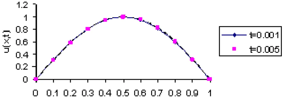
To solve Burgers’ equation for very small kinematics viscosity (i.e. very high Reynolds number) is a di¢ cult work both analytically, due to slow convergence of the in…nite series [2], and numerically in which methods computers’ mem-ory requirements are very high. However, we have obtained series solution for 0 < t < 0:005 by calculating the series coe¢ cients in a di¤erent way by means of di¤erential transformation method. For small values of t; the solution of (20) which is subjected to initial and boundary conditions (21)-(22) have been cal-culated easily. Figure1 shows the solution for = 1 and t = 0:001; 0:005. There is no signi…cant di¤erence for di¤erent values of t except x = 0:5. However, by decreasing the value of kinematics viscosity from = 1 to = 0:001, we observe that two solutions for both t = 0:001; 0:005 are almost the same (see Figure 2). It states that the solution is not a¤ected by decreasing for small values of t: On the other hand, a further work can be done by the same method in order to hold whole solution domain. This can be overwhelmed by using any mathemat-ical software such as Maple, Mathematica, or any programming languages. As a result, it can be said that the method, the di¤erential transform, is a useful and easy tool in order to obtain closed or approximate solutions for linear or nonlinear partial di¤erential equations
Figure 1: Solutions of (20)-(22) for = 0:001 and t = 0:001; 0:005
Figure 2: Solutions of (20)-(22) for = 0:001 and t = 0:001; 0:005
References
1. Burger J.M. (1948): A mathematical Model Illustrating the Theory of Turbulence, Academic Press, New York, .
2. Cole J.D. (1951): On a quasilinear parabolic equations occurring in aerodynamics, Quart. Appl. Math. 9, 225-236
3. Benton E., Platzman G.W. (1972): A table of solutions of the on-dimensional Burgers’ equation,Quart. Appl. Math. 30 195-212
4. Kutluay S., Bahad¬r A.R., Özde¸s A. (1999): Numerical solution of one-dimensional Burgers’equation: Explicit and exact-implicit …nite di¤ erence methods, J. Comput. Appl. Math.103, 251-261
5. Özi¸s T., Özde¸s N. (1996): A direct variational method to Burgers’ equation, J. Comput. Appl.Math. 71 163- 175.
6. Pukhov G.E. (1986): Di¤ erential transformations and mathematical modeling of physical processes, Kiev.
7. Chen C.K. , Ho S.H. (1999): Solving partial di¤ erential equations by two dimensional di¤ erential transform method, Appl. Math. Comput.106, 171-179
8. Jang M.J., Chen, C.L. Liu Y.C.(2001): Two-dimensional di¤ erential transform for partial di¤ erential equations, Appl.Math.Comput 121, 261-270.
9. Ayaz F. (2003): On the two dimensional di¤ erential transform method, Appl. Math. Comput. 143, 361-374.
10. Ayaz F. (2004): Solutions of the system of di¤ erential equations by di¤ erential transform method, Appl. Math. Comput. 147 547-567.
11. Kaya D., Yokus A. (2002): A numerical comparison of partial solutions in the de-composition method for linear and nonlinear partial di¤ erential equations, Maths.Comput. Simul., 60 507-512.