Estimating the Parameters of Xgamma Weibull Distribution
Kadir KARAKAYA1,*, Caner TANIŞ2
1Selçuk University, Science Faculty, Department of Statistics, Konya, Turkey
[email protected], ORCID: 0000-0002-0781-3587
2Çankırı Karatekin University, Science Faculty, Department of Statistics, Çankırı, Turkey
[email protected], ORCID: 0000-0003-0090-1661
Received: 15.08.2020 Accepted: 02.12.2020 Published: 30.12. 2020
Abstract
In this paper, we consider a comparison of estimation methods for the parameters of Xgamma Weibull distribution. It is discussed five different estimation methods such as maximum likelihood method, least-squares method, weighted least-squares method, the method of Anderson-Darling and the method of Crámer–von-Mises. We compare these estimators via Monte Carlo simulations according to the biases and mean-squared errors (MSEs). Further, seven real data applications are conducted and Kolmogorov Smirnov goodness of fit test is also calculated for all estimators.
Keywords: Xgamma Weibull distribution; Maximum likelihood method; Least-squares method; Weighted least-squares method; Anderson-Darling method; Crámer–von-Mises estimation method.
Xgamma Weibull Dağılımının Parametre Tahmini Öz
Bu çalışmada, Xgamma Weibull dağılımının parametre tahmini için tahmin yöntemlerinin kıyaslanması problemi ele alınmıştır. En çok olabilirlik yöntemi, en küçük kareler yöntemi,
yöntemi olmak üzere beş tahmin yöntemi incelenmiştir. Bu beş tahmin yöntemini yan ve hata kareler ortalaması açısından karşılaştırabilmek için bir Monte Carlo simülasyon çalışması yapılmıştır. Ayrıca yedi gerçek veri uygulaması yapılmış ve tüm tahmin ediciler için Kolmogorov Smirnov uyum iyiliği testi hesaplanmıştır.
Anahtar Kelimeler: Xgamma Weibull dağılımı; En çok olabilirlik yöntemi; En küçük kareler yöntemi; Ağırlıklandırılmış en küçük kareler yöntemi; Anderson-Darling yöntemi; Crámer–von-Mises yöntemi.
1. Introduction
Xgamma Weibull distribution was suggested by Yousof et al. in [1] as an alternative Weibull distribution. We denote Xgamma Weibull distribution as . The probability density function (pdf) and cumulative density function (cdf) of distribution are
(1)
and
(2)
respectively, where is a scale parameter, is a shape parameter and is an indicator function. In [1], the authors examined some of the statistical properties of
distribution. Yousof et al. [1] concluded that the shape of failure rate function of distribution can be increasing, decreasing and bathtub. It was also stated that
distribution can be applied for modelling data in economics, medicine, engineering, reliability etc [1].
It is extensively preferred comparison of the methods of estimation regarding distribution by many authors. It is well-known that the generalized exponential distribution is studied in terms of different estimation methods in [2]. In [3], the authors introduced the generalized Rayleigh distribution and also compared the methods of different estimation for this distribution. The different methods of estimation for half-logistic distribution were compared in [4]. Mazucheli et al. [5] examined different estimation methods for weighted Lindley distribution. Different
( )
q
, XGW b( )
q
, XGW b(
) ( )
( )( )
2 1 2 0, 1 ; , 1 , 1 2 q q q q q - -¥ æ ö = ç + ÷ + è ø b b x b b f x b x e x I x(
; ,)
1 1 2 2(
)
, 2 1 q q q q q q -æ ö = - + +ç + ÷ + è ø b b x b x e F x b x 0 q > b>0 I(0,¥)( )
x( )
q
, XGW b( )
q
, XGW b( )
q
, XGW bmethods of estimation for two parameter Rayleigh distribution are discussed in [6]. Peng and Yan [7] obtained maximum likelihood estimators and Bayesian estimators for the parameters of an extended Weibull distribution. A new alternative distribution to Weibull distribution was suggested in [8]. The authors also discussed some properties and different estimation methods such as maximum likelihood, ordinary and weighted least squares, percentile and maximum product spacing this new distribution in [8]. The methods of estimation for log-Kumaraswamy distribution were studied in [9]. Afify et al. [10] considered different methods of estimation for Weibull Marshall-Olkin Lindley distribution.
The main purpose of this paper is to compare five different estimators for the parameters of the distribution via Monte Carlo simulations and real data applications. Thus, maximum likelihood estimators (MLEs), least square estimators (LSEs), weighted least square estimators (WLSEs), Anderson-Darling estimators (ADEs) and Crámer–von-Mises estimators (CVMEs) are considered for point estimation. The rest of this study is organized as follows: Section 2 introduces five different methods of estimation. A comprehensive Monte Carlo simulation study is presented in order to evaluate the performances of these estimators according to MSE criteria in Section 3. In Section 4, we consider real data illustrations. Finally, concluding remarks are given in Section 5.
2. Point estimations on model parameters
In this section, we focus on five estimators for estimating the unknown parameters of distribution. For this purpose, we examine the maximum likelihood method, least-squares method, weighted least least-squares method, the method of Crámer–von-Mises and the method of Anderson-Darling.
Let be a random sample from the distribution and represent the corresponding order statistics. Additionally, denotes the observed value of . Based on this information the likelihood and log-likelihood function of the distribution are given, respectively, by
(3)
( )
q
, XGW b( )
q
, XGW b 1, 2, ,! n X X X XGW( )
q
,b ( )1 < ( )2 <!< ( )n X X X x( )i ( )i X( )
q
, XGW b( )
(
2)
1 2 1 1 1 1 2 q q q q -= æ ö = ç + ÷ + è øÕ
b i n x b b i i i b L Ψ x e x(4)
where
Then, MLEs of is given by
(5) Let us define the following functions which are useful to obtain the different type of estimators:
and
The LSEs, WLSEs, CvMEs and ADEs of the parameter are given, respectively, by
(6) (7) (8)
( )
( )
( )
(
) (
)
( )
2 1 1 1 1log 2 log log 1 1 log log 1
2 q q q q = = = æ ö = + - + + - - + ç + ÷ è ø
å
å
å
! n n b n b i i i i i i n b n n b x x x Ψ( )
q
, .
=
b
Ψ
Ψ( )
{
}
1 ˆ =arg max ! . Ψ Ψ Ψ( )
( ) ( ) ( )(
)
( )
(
(
)(
)
)
( ) ( ) ( )(
)
( )
( ) ( ) ( )(
)
2 2 2 1 2 2 2 2 1 2 2 1 1 , 2 1 1 2 1 1 1 , 1 2 1 1 1 1 1 12 2 1 q q q q q q q q q q q q q q q -= -= -æìï æ ö üï ö ç ç ÷ ÷ = í - + + + ý -ç ÷ çïî è ø + ïþ + ÷ è ø æì æ ö ü ö + + çï ç ÷ ï ÷ = í - + + + ý -ç ÷ ç ÷ - + ïî è ø + ïþ + è ø æ ö ç ÷ = + - + + + ç ÷ + è øå
å
b i b i b i b x n i b LS i i b x n i b WLS i i b x i b CvM i x e i Q x n x n n e i Q x i n i n x e Q x n Ψ Ψ Ψ 2 1 2 1 2 = æìï üï - ö çí ý- ÷ çïî ïþ ÷ è øå
n i i n( )
(
)
( ) ( ) ( )(
)
( ) ( ) ( )(
)
2 2 1 2 2 1 2 1 log 1 1 1 2 1 1 log 1 . 2 1 q q q q q q q q q q -= -= æ æìï æ ö üïöö ç - çí - + +ç + ÷ ý÷÷ ç ÷ ç ÷ = - - çïî è ø + ïþ÷ è ø è ø æ æìïæ ö üïöö ç ç ç ÷ ÷÷ + í + + + ý ç ÷ ç çïîè ø + ïþ÷÷ è ø è øå
å
b i b i b x i b n i AD i b x n i b i i x e i x Q n n x e x n Ψ Ψ( )
{
}
2 ˆ =arg min , LS Q Ψ Ψ Ψ( )
{
}
3 ˆ =arg min , WLS Q Ψ Ψ Ψ( )
{
}
4 ˆ =arg min , CvM Q Ψ Ψ Ψ(9) All estimators given in Eqn. (5)-(9) can be achieved by optim function in R with BFGS algorithm.
3. Simulation Study
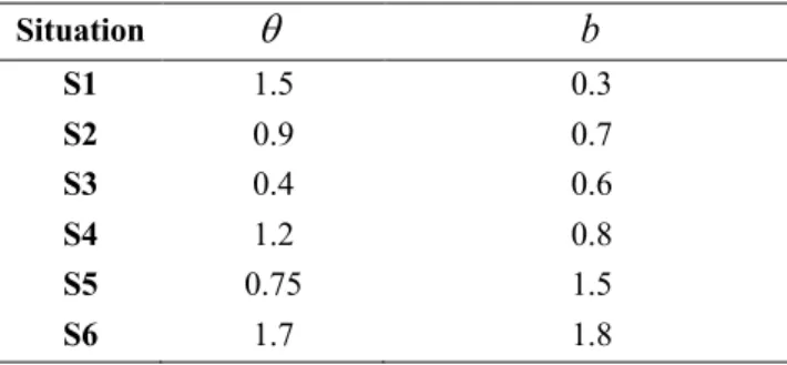
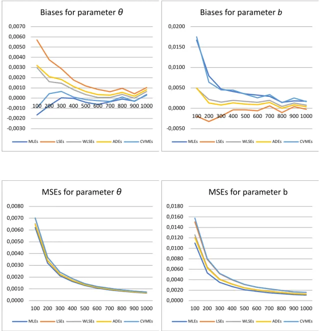
In this section, we consider a Monte Carlo simulation study to interpret the biases and MSEs of MLEs, LSEs, WLSEs, CvMEs and ADEs of XGW distribution parameters are estimated with 5000 trials. The acceptance-rejection algorithm is used to generate the data from distribution. BFGS algorithm is carried out to get the five estimates given in (5)-(9). The simulation results are summarized via Figs. 1-6. Table 1 provides six parameter settings for Monte Carlo simulations. In Figs. 1-6, the biases and MSEs of MLEs, LSEs, WLSEs, CVMEs and ADEs are reported.
In the simulation study, the samples of sizes are considered as n=100, 200, 300, 400, 500, 600, 700, 800, 900, 1000.
Table 1: Parameter settings using from simulation study Situation S1 1.5 0.3 S2 0.9 0.7 S3 0.4 0.6 S4 1.2 0.8 S5 0.75 1.5 S6 1.7 1.8
( )
{
}
5 ˆ =arg min . AD Q Ψ Ψ Ψ( )
,
XGW
q
b
q
b
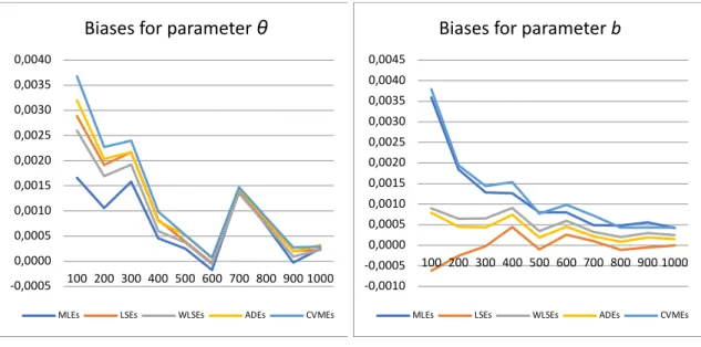
Figure 1: Biases and MSEs for situation S1 -0,0005 0,0000 0,0005 0,0010 0,0015 0,0020 0,0025 0,0030 0,0035 0,0040 100 200 300 400 500 600 700 800 900 1000
Biases for parameter θ
MLEs LSEs WLSEs ADEs CVMEs
-0,0010 -0,0005 0,0000 0,0005 0,0010 0,0015 0,0020 0,0025 0,0030 0,0035 0,0040 0,0045 100 200 300 400 500 600 700 800 900 1000
Biases for parameter b
MLEs LSEs WLSEs ADEs CVMEs
0,0000 0,0020 0,0040 0,0060 0,0080 0,0100 0,0120 0,0140 0,0160 0,0180 100 200 300 400 500 600 700 800 900 1000
MSEs for parameter θ
MLEs LSEs WLSEs ADEs CVMEs
0,0000 0,0001 0,0002 0,0003 0,0004 0,0005 0,0006 0,0007 0,0008 0,0009 100 200 300 400 500 600 700 800 900 1000
MSEs for parameter b
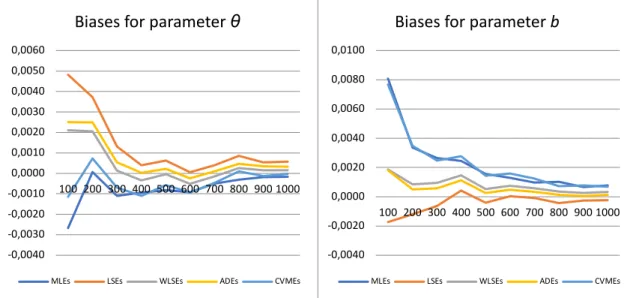
Figure 2: Biases and MSEs for situation S2 -0,0040 -0,0030 -0,0020 -0,0010 0,0000 0,0010 0,0020 0,0030 0,0040 0,0050 0,0060 100 200 300 400 500 600 700 800 900 1000
Biases for parameter θ
MLEs LSEs WLSEs ADEs CVMEs
-0,0040 -0,0020 0,0000 0,0020 0,0040 0,0060 0,0080 0,0100 100 200 300 400 500 600 700 800 900 1000
Biases for parameter b
MLEs LSEs WLSEs ADEs CVMEs
0,0000 0,0010 0,0020 0,0030 0,0040 0,0050 0,0060 0,0070 0,0080 0,0090 0,0100 100 200 300 400 500 600 700 800 900
MSEs for parameter θ
MLEs LSEs WLSEs ADEs CVMEs
0,0000 0,0005 0,0010 0,0015 0,0020 0,0025 0,0030 0,0035 0,0040 100 200 300 400 500 600 700 800 900 1000
MSEs for parameter b
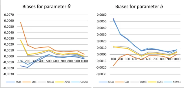
Figure 3: Biases and MSEs for situation S3 -0,0030 -0,0020 -0,0010 0,0000 0,0010 0,0020 0,0030 0,0040 0,0050 0,0060 0,0070 100 200 300 400 500 600 700 800 900 1000
Biases for parameter θ
MLEs LSEs WLSEs ADEs CVMEs
-0,0030 -0,0020 -0,0010 0,0000 0,0010 0,0020 0,0030 0,0040 0,0050 0,0060 100 200 300 400 500 600 700 800 900 1000
Biases for parameter b
MLEs LSEs WLSEs ADEs CVMEs
0,0000 0,0005 0,0010 0,0015 0,0020 0,0025 0,0030 0,0035 0,0040 100 200 300 400 500 600 700 800 900 1000
MSEs for parameter θ
MLEs LSEs WLSEs ADEs CVMEs
0,0000 0,0005 0,0010 0,0015 0,0020 0,0025 100 200 300 400 500 600 700 800 900 1000
MSEs for parameter b
Figure 4: Biases and MSEs for situation S4 -0,0030 -0,0020 -0,0010 0,0000 0,0010 0,0020 0,0030 0,0040 0,0050 0,0060 0,0070 100 200 300 400 500 600 700 800 900 1000
Biases for parameter θ
MLEs LSEs WLSEs ADEs CVMEs
-0,0030 -0,0020 -0,0010 0,0000 0,0010 0,0020 0,0030 0,0040 0,0050 0,0060 100 200 300 400 500 600 700 800 900 1000
Biases for parameter b
MLEs LSEs WLSEs ADEs CVMEs
0,0000 0,0020 0,0040 0,0060 0,0080 0,0100 0,0120 0,0140 100 200 300 400 500 600 700 800 900 1000
MSEs for parameter θ
MLEs LSEs WLSEs ADEs CVMEs
0,0000 0,0010 0,0020 0,0030 0,0040 0,0050 0,0060 100 200 300 400 500 600 700 800 900 1000
MSEs for parameter b
Figure 5: Biases and MSEs for situation S5 -0,0030 -0,0020 -0,0010 0,0000 0,0010 0,0020 0,0030 0,0040 0,0050 0,0060 0,0070 100 200 300 400 500 600 700 800 900 1000
Biases for parameter θ
MLEs LSEs WLSEs ADEs CVMEs
-0,0050 0,0000 0,0050 0,0100 0,0150 0,0200 100 200 300 400 500 600 700 800 900 1000
Biases for parameter b
MLEs LSEs WLSEs ADEs CVMEs
0,0000 0,0010 0,0020 0,0030 0,0040 0,0050 0,0060 0,0070 0,0080 100 200 300 400 500 600 700 800 900 1000
MSEs for parameter θ
MLEs LSEs WLSEs ADEs CVMEs
0,0000 0,0020 0,0040 0,0060 0,0080 0,0100 0,0120 0,0140 0,0160 0,0180 100 200 300 400 500 600 700 800 900 1000
MSEs for parameter b
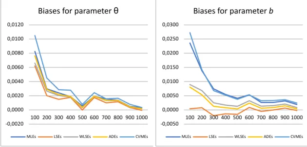
Figure 6: Biases and MSEs for situation S6
From Figs. 1-6, it can be concluded that the biases and MSEs of all estimates are close to zero when the sample of size increases. Also, the best estimator is maximum likelihood estimator for parameter b according to MSE criterion. It is quite difficult to comment on the parameter because the MSEs of the estimators are very close to each other. On the other hand, when looking at the values of biases estimators MLEs and LSEs are substantial for the parameter b, while MLEs and CVMEs for the parameter draw attention because of their good results. In other words, MLEs and CVMEs for the parameter, MLEs and LSEs for the b parameter gave more unbiased
-0,0020 0,0000 0,0020 0,0040 0,0060 0,0080 0,0100 0,0120 100 200 300 400 500 600 700 800 900 1000
Biases for parameter θ
MLEs LSEs WLSEs ADEs CVMEs
-0,0050 0,0000 0,0050 0,0100 0,0150 0,0200 0,0250 0,0300 100 200 300 400 500 600 700 800 900 1000
Biases for parameter b
MLEs LSEs WLSEs ADEs CVMEs
0,0000 0,0050 0,0100 0,0150 0,0200 0,0250 100 200 300 400 500 600 700 800 900 1000
MSEs for parameter θ
MLEs LSEs WLSEs ADEs CVMEs
0,0000 0,0050 0,0100 0,0150 0,0200 0,0250 0,0300 0,0350 100 200 300 400 500 600 700 800 900 1000
MSEs for parameter b
MLEs LSEs WLSEs ADEs CVMEs
q
q
q
4. Real Data Applications
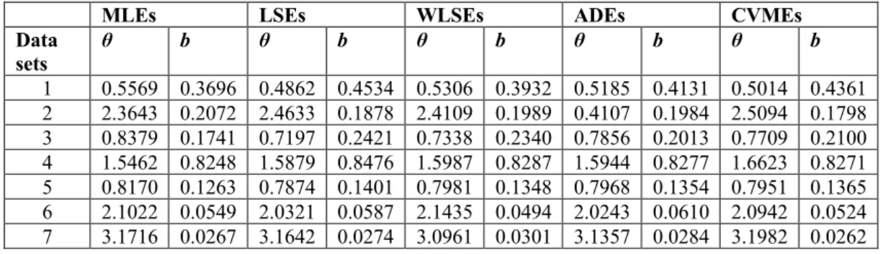
In this section, seven real data applications for the XGW distribution are studied. Also, five estimation methods are compared for XGW distribution in this data modelling. The MLEs, LSEs, WLSEs, ADEs and CVMEs of the parameters of XGW distribution are obtained by BFGS algorithm and reported in Table 2. Kolmogorov-Smirnov statistics (KS) and related p values are given in Table 3 for all estimators. From Tables 2-3 it is observed that all estimators nearly give the same results. Therefore, if one will use the XGW distribution in real data modeling, they can use one of the five estimation methods investigated in this paper.
In the following we give the seven real data sets; Data Set 1 ([11]) 65, 156, 100, 134, 16, 108, 121, 4, 39, 143, 56, 26, 22, 1, 1, 5, 65, 56, 65, 17, 7, 16, 22, 3, 4, 2, 3, 8, 4, 3, 30, 4, 43. Data Set 2 ([12]) 0.39, 0.85, 1.08, 1.25, 1.47, 1.57, 1.61, 1.61, 1.69, 1.80, 1.84, 1.87, 1.89, 2.03, 2.03, 2.05, 2.12, 2.35, 2.41, 2.43, 2.48, 2.50, 2.53, 2.55, 2.55, 2.56, 2.59, 2.67, 2.73, 2.74, 2.79, 2.81, 2.82, 2.85, 2.87, 2.88, 2.93, 2.95, 2.96, 2.97, 3.09, 3.11, 3.11, 3.15, 3.15, 3.19, 3.22, 3.22, 3.27, 3.28, 3.31, 3.31, 3.33, 3.39, 3.39, 3.56, 3.60, 3.65, 3.68, 3.70, 3.75, 4.20, 4.38, 4.42, 4.70, 4.90. Data Set 3 ([13]) 1.4, 5.1, 6.3, 10.8, 12.1, 18.5, 19.7, 22.2, 23, 30.6, 37.3, 46.3, 53.9, 59.8, 66.2. Data Set 4 ([14]) 0.77, 1.74, 0.81, 1.20, 1.95, 1.20, 0.47, 1.43, 3.37, 2.20, 3.00, 3.09, 1.51, 2.10, 0.52, 1.62, 1.31, 0.32, 0.59, 0.81, 2.81, 1.87, 1.18, 1.35, 4.75, 2.48, 0.96, 1.89, 0.90, 2.05. Data Set 5 ([15]) 0.3, 0.3, 4.0, 5.0, 5.6, 6.2, 6.3, 6.6, 6.8, 7.4, 7.5, 8.4, 8.4, 10.3, 11.0, 11.8, 12.2, 12.3, 13.5, 14.4, 14.4, 14.8, 15.5, 15.7, 16.2, 16.3, 16.5, 16.8, 17.2, 17.3, 17.5, 17.9, 19.8, 20.4, 20.9, 21.0, 21.0, 21.1, 23.0, 23.4, 23.6, 24.0, 24.0, 27.9, 28.2, 29.1, 30.0, 31.0, 31.0, 32.0, 35.0, 35.0, 37.0, 37.0, 37.0, 38.0, 38.0, 38.0, 39.0, 39.0, 40.0, 40.0, 40.0, 41.0, 41.0, 41.0, 42.0, 43.0, 43.0, 43.0, 44.0, 45.0, 45.0, 46.0, 46.0, 47.0, 48.0, 49.0, 51.0, 51.0, 51.0, 52.0, 54.0, 55.0, 56.0, 57.0, 58.0, 59.0, 60.0, 60.0, 60.0, 61.0, 62.0, 65.0, 65.0, 67.0, 67.0, 68.0, 69.0, 78.0, 80.0,83.0, 88.0, 89.0, 90.0, 93.0, 96.0, 103.0, 105.0, 109.0, 109.0, 111.0, 115.0, 117.0, 125.0, 126.0, 127.0, 129.0, 129.0, 139.0, 154.0.
Data Set 6 ([16]) 1.6, 3.5, 4.8, 5.4, 6.0, 6.5, 7.0, 7.3, 7.7, 8.0, 8.4, 2.0, 3.9, 5.0, 5.6, 6.1, 6.5, 7.1, 7.3, 7.8, 8.1, 8.4, 2.6, 4.5, 5.1, 5.8, 6.3, 6.7, 7.3, 7.7, 7.9, 8.3, 8.5, 3.0, 4.6, 5.3, 6.0, 8.7, 8.8, 9.0. Data Set 7 ([17]) 2.247, 2.64, 2.842, 2.908, 3.099, 3.126, 3.245, 3.328, 3.355, 3.383, 3.572, 3.581, 3.681,3.726, 3.727, 3.728, 3.783, 3.785, 3.786, 3.896, 3.912, 3.964, 4.05, 4.063, 4.082,4.111, 4.118, 4.141, 4.216, 4.251, 4.262, 4.326, 4.402, 4.457, 4.466, 4.519, 4.542,4.555, 4.614,4.632, 4.634, 4.636, 4.678, 4.698, 4.738, 4.832, 4.924, 5.043, 5.099, 5.134, 5.359, 5.473, 5.571, 5.684, 5.721, 5.998, 6.06.
Table 2: Parameter estimation for all real data sets based on the all estimators
MLEs LSEs WLSEs ADEs CVMEs
Data sets θ b θ b θ b θ b θ b 1 0.5569 0.3696 0.4862 0.4534 0.5306 0.3932 0.5185 0.4131 0.5014 0.4361 2 2.3643 0.2072 2.4633 0.1878 2.4109 0.1989 0.4107 0.1984 2.5094 0.1798 3 0.8379 0.1741 0.7197 0.2421 0.7338 0.2340 0.7856 0.2013 0.7709 0.2100 4 1.5462 0.8248 1.5879 0.8476 1.5987 0.8287 1.5944 0.8277 1.6623 0.8271 5 0.8170 0.1263 0.7874 0.1401 0.7981 0.1348 0.7968 0.1354 0.7951 0.1365 6 2.1022 0.0549 2.0321 0.0587 2.1435 0.0494 2.0243 0.0610 2.0942 0.0524 7 3.1716 0.0267 3.1642 0.0274 3.0961 0.0301 3.1357 0.0284 3.1982 0.0262 Table 3: Kolmogrov-Smirnov statistics and related p value for all real data sets based on the all estimators
MLEs LSEs WLSEs ADEs CVMEs
Data
sets KS p value KS p value KS p value KS p value KS p value
1 0.1258 0.6723 0.1213 0.7158 0.1152 0.7733 0.1052 0.8584 0.1143 0.7814 2 0.0718 0.8853 0.0631 0.9551 0.0647 0.9445 0.0661 0.9347 0.0586 0.9769 3 0.0999 0.9945 0.1051 0.9901 0.0971 0.9961 0.0974 0.9960 0.0968 0.9963 4 0.0860 0.9793 0.0737 0.9967 0.0674 0.9992 0.0674 0.9992 0.0735 0.9968 5 0.0580 0.8095 0.0613 0.7534 0.0592 0.7887 0.0592 0.7895 0.0611 0.7568 6 0.1092 0.7263 0.1098 0.7202 0.0934 0.8756 0.1016 0.8031 0.1017 0.8019 7 0.0645 0.9590 0.0557 0.9900 0.0634 0.9647 0.0619 0.9713 0.0529 0.9946 5. Concluding Remarks
In this study, XGW distribution introduced by [1] is investigated with regard to some point estimations. Five estimators are examined to estimate the two parameters of XGW distribution. A new extension is ensured for the estimation of the parameters for XGW distribution. Monte Carlo simulations are carried out for six different parameter values and different sample sizes. It is eventuated that when the sample of sizes increases, the biases and MSEs of all estimators decreases and approach to zero. The parameter estimates and KS of XGW distribution are
References
[1] Yousof, H.M., Korkmaz, M.Ç., Sen, S., A new two-parameter lifetime model, Annals of Data Science, 2020, DOI: 10.1007/s40745-019-00203-w.
[2] Gupta, R.D., Kundu, D., Generalized exponential distribution: different method of
estimations, Journal of Statistical Computation and Simulation, 69(4), 315-337, 2001.
[3] Kundu, D., Raqab, M.Z., Generalized Rayleigh distribution: different methods of
estimations, Computational statistics & data analysis, 49(1), 187-200, 2005.
[4] Asgharzadeh, A., Rezaie, R., Abdi, M., Comparisons of methods of estimation for the
half-logistic distribution, Selçuk Journal of Applied Mathematics, 93-108, 2011.
[5] Mazucheli, J., Louzada F., Ghitany M.E., Comparison of estimation methods for the
parameters of the weighted Lindley distribution, Applied Mathematics and Computation, 220,
463-471, 2013.
[6] Dey, S., Dey, T., Kundu, D., Two-parameter Rayleigh distribution: different methods
of estimation, American Journal of Mathematical and Management Sciences, 33(1), 55-74, 2014.
[7] Peng, X., Yan, Z., Estimation and application for a new extended Weibull distribution, Reliability Engineering & System Safety, 121, 34-42, 2014.
[8] Nassar, M., Afify, A.Z., Dey, S., Kumar, D., A new extension of Weibull distribution:
properties and different methods of estimation, Journal of Computational and Applied
Mathematics, 336, 439-457, 2018.
[9] Taniş, C., Saracoglu, B., Comparisons of six different estimation methods for
log-kumaraswamy distribution, Thermal Science, 23, 1839-1847, 2019.
[10] Afify, A.Z., Nassar, M., Cordeiro, G. M., Kumar, D., The Weibull Marshall–Olkin
Lindley distribution: properties and estimation, Journal of Taibah University for Science, 14(1),
192-204, 2020.
[11] Feigl, P., Zelen, M., Estimation of exponential survival probabilities with concomitant
information, Biometrics 21, 826–38, 1965.
[12] Nichols, M.D., Padgett, W.J., A bootstrap control chart for Weibull percentiles, Quality and Reliability Engineering International, 22, 141-151, 2006.
[13] Lawless, J.F., Statistical models and methods for lifetime data, Wiley, New York, 2003.
[14] Bjerkedal, T., Acquisition of resistance in Guinea Piesinfected with different doses of
Virulent Tubercle Bacill, American Journal of Hygiene, 72, 130-148 , 1960.
[15] Lee, E.T., Statistical methods for survival data analysis, John Wiley, New York, 1992. [16] Xu, K., Xie, M., Tang, L.C., Ho, S.L., Application of neural networks in forecasting
[17] Crowder, M.J., Kimber, A.C., Smith, R.L., Sweeting, T.J. The statistical analysis of