Adıyaman Üniversitesi
Fen Bilimleri Dergisi 2 (1) (2012) 24-33
The Stability Analysis Depending Number of Predation in Discrete-Time Population Model and Allee Effect
Hasan Köse1, Özlem Ak Gümüş2*
1
Selçuk Üniversitesi, Fen Fakültesi, Matematik Bölümü, Konya
2
Adıyaman Üniversitesi, Fen Edebiyat Fakültesi, Matematik Bölümü, Adıyaman
Abstract
In this paper, the stability analysis has been investigated by changing only the function )
(Nt
g in the discrete-time population models as follows
1 ( ) ( ) ( , )
t t t t t t t
N N N f N N g N F N . In fact, the authors Merdan and Duman have
studied similar subject for different constants and function. In our case, this model has faster convergence and stable than the previous model under our assumptions ong(Nt). We also observe that stability has been significantly increased in the model, when Allee effect is considered.
Keywords: Allee effect, stability analysis, discrete-time model.
Fark Zamanlı Popülasyon Modelinde Avcı Sayısına Bağlı Olarak Kararlılık Analizi ve Allee Etkisi
Özet
Bu çalışmada, sadece g(Nt) fonksiyonunu değiştirerek,
1 ( ) ( ) ( , )
t t t t t t t
N N N f N N g N F N fark zamanlı popülasyon modelinin kararlılık
25
benzer konuda çalıştılar. Bizim durumumuzda g(Nt) üzerindeki varsayımlarımız altında bu model, önceki modelden daha hızlı kararlılığa ve yakınsamaya sahiptir. Biz aynı zamanda, Allee etkisi göz önüne alındığında modelin kararlılığının önemli bir şekilde arttığı gözlemledik.
Anahtar kelimeler:Allee etkisi, kararlılık analizi, fark zamanlı model.
Introduction
In recent years, the study of the stability in population dynamics have been an attractive search area. In these studies, most of the models have been constructed under the assumption of asexually reproducing organism. Such population dynamics models exhibit complexity in their movements. The general conclusion of these studies show that models are not structurally stable. This situation encouraged many scientists to modify the models and to develop better parameter estimation procedures [1-3].
According to the studies performed on different populations, sexually reproducing decreases the variations in the intensity of individual genotypes, and eventually increases the dynamic stability of the model. This situation is a conclusion of increasing parameter number [4].
Although Allee Effect may delay the stability in some population dynamics, it generally accelerates the stability of the models [5-10].
Merdan and Duman [5], have studied the stability of the following difference equation that involves predation effect at low population density,
1 ( ) ( ) ( , )
t t t t t t t
N N N f N N g N F N (1) and that equation with Allee Effect,
* *
1 ( ) ( ) ( ) ( , )
t t t t t t t t
N N N N f N N g N F N (2) where N is the density at time t, t is the per capita growth rate, and f(Nt) is the function
describing interactions among the individuals. They showed that when the population models given by Eq. (1) is subject to an Allee effect, stability of the equilibrium points increases. For
,
f g and functions, we write,
1)
26
2)
f for N (0, ) , f N( )0
3)
f f N( ) has at least one positive root. 1) g for g(0)=0 and N (0, ) , 0 g N( ) 2) g lim ( ) 0 N g N 3)
g g N( c) , 0 N c (0, ) has only one critical value. 1) a If N=0, then ( )N 0 2) a for N (0, ) , ( )N 0 3) a lim ( ) 1 N N
Now, we will give some theorems and results that is required later in this study.
Theorem 1.1: Assume that a positive equilibrium point N* of Eq. (1) exist. Then it is locally stable if * * * * * 2 ( ) ( ) 0 ( ) ( ) ( ) f N g N N g N f N g N holds [5].
Result 1.1: Let N* be a positive equilibrium point of Eq. (1). Then we have three possible cases [5]:
i) If N*Nc , then the sufficient condition to make N* unstable is,
* * * * * * ( ) ( ) 2 ( ) ( ) ( ) f N g N f N g N N g N
ii) If N* Nc, then it is unstable if and only if
* * * * ( ) 2 ( ) ( ) f N f N N g N iii) If N* Nc, then it is unstable if and only if
* * * * * * ( ) ( ) 2 ( ) ( ) ( ) f N g N f N g N N g N or * * * * ( ) ( ) ( ) ( ) f N g N f N g N .
Theorem 1.2: Assume that a positive equilibrium point N*of Eq. (2) exists. Then, it is locally stable if * * * * * * * * 2 ( ) ( ) ( ) 0 ( ) ( ) ( ) ( ) N f N g N N g N N f N g N
27 satisfied [5].
Result 1.2: Let N* be a positive equilibrium point of Eq. (1) satisfying N * (0,Nc], where g has only one critical point on ( 0, ), that is, there is only one point Nc( 0, ) such that
0 )
(
Nc
g [5]. Then, Theorem 1 and Corallary 1 (i)-(ii) imply that N* is unstable if and only if F(,N*)1 [5]. On the other hand, since
* * ( ) ( ) N N
is always positive, then we write
* * *
( , ) ( , )
F N F N [5].
Result 1.3: The Allee effect in Eq. (2) increases the local stability of the equilibrium point
*
N of Eq. (1) provided that N* Nc [5]. Main results
The main purpose of this study is to examine the stability of Eq. (1) and Eq. (2) with the choice of 1 1 1 ) ( 2 t t t t N N N N g for N (0, ) , K=1 and K N N f t t 1 ) ( , whereas
Merdan and Duman [5] examined the same problem by taking g(Nt) as,
2 ( ) . 1 t t t N g N N (3) They obtained respectively following equations from Eq. (1) and Eq. (2) respectively,
2 1 (1 ) 2 1 t t t t t t N N N N N K N (4) 2 2 * 1 (1 ) 2 1 t t t t t t t N N N N N N K N (5) where ve 0 ) ( * * N .
Now, if we consider the new form of g(Nt) as,
1 1 1 ) ( 2 t t t t N N N N g (6)
28 2 1 (1 ) 2 1 1 t t t t t t t t N N N N N N K N N (7) 2 2 ** 1 (1 ) 1 2 1 t t t t t t t t t N N N N N N N K N N (8) where and 0 ) ( ** * * N
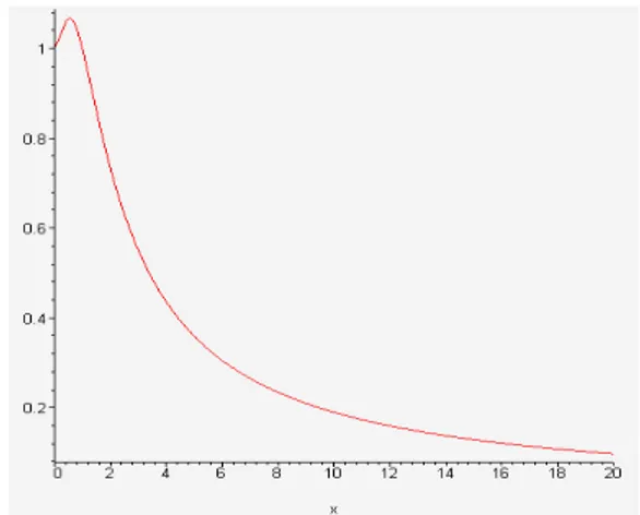
. The comparison of the results of the previous and the proposed models for g(Nt) is shown in Figure 1.
Figure 1.a. The graph of the function (3). Figure 1.b. The graph of the function(6).
Population movement for a certain
By using Matlab package programming language, we can obtain Figure 2 from Eq. (7) and Eq. (8) respectively for 2.33and K=1. Then, results from Eq. (4) and Eq. (5) are shown in Figure 3 respectively.
29
Figure 2.b. The graph of Model (8), for ** 2.5450, N0 0.4 and 0.05
Figure 3.a.The graph of Model (4), for 2.33 and N0 0.6
Figure 3.b. The graph of Model (5), for * 2.9190
30 Population movements for new model
For 2.5 and K=1, we obtain respectively Figure 4.a and Figure 4.b from Eq. (7) and Eq. (8) and obtain respectively Figure 5.a and Figure 5.b from Eq. (4) and Eq. (5).
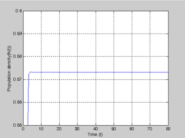
Figure 4.a. The graph of Model (7), for 2.5and N 0 0.4
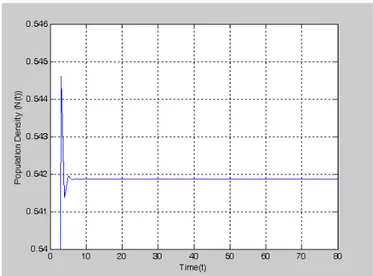
Figure 4.b. The graph of Model (8), for **
2.37235,
N 0 0.4 and 0.2
31 Figure 5.b. The graph of Model (5), for *
3.3111,
N 0 0.6 and 0.2
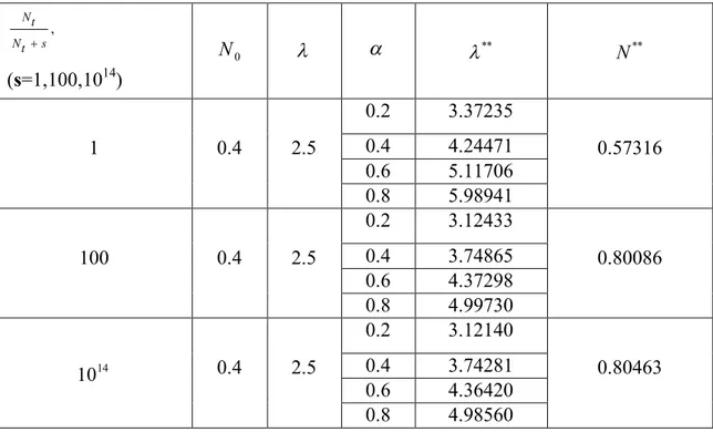
In the following table (see Table 1 below), it is seen that the comparison of the population movements for different parameters. In fact, while s , the function (6)
converges to the function (3). Therefore, it can be concluded that the behavior of the model (7) and (8) in our interest converges to that of (4) and (5).
Table 1. Equilibrium points values according to certain values of , and s for N initial 0
conditions , Nt Nt s (s=1,100,1014) 0 N ** N** 1 0.4 2.5 0.2 3.37235 0.57316 0.4 4.24471 0.6 5.11706 0.8 5.98941 100 0.4 2.5 0.2 3.12433 0.80086 0.4 3.74865 0.6 4.37298 0.8 4.99730 14 10 0.4 2.5 0.2 3.12140 0.80463 0.4 3.74281 0.6 4.36420 0.8 4.98560
32 0 N , Nt Nt s (s=1,100,1014) ** N** 0.4 0.05 2.33 1 2.545 0.54187 100 2.478 0.78715 14 10 2.477 0.79116 2.43 1 2.647 0.56077 100 2.583 0.79543 14 10 2.582 0.79930 Discussion
In this study, we investigated the stability of the model under a different choice of the function which increases the number of predators. We compared the stability of the models with different predator functions by the corresponding graphs. We also observed the behavior of the model with Allee effect. In addition to, we have also observed the changes in the model with low population density and with low Allee constant. It is interesting that even with low population density and high Allee effect, there is no extinction. However, it reaches to the equilibrium point faster.
0 N , Nt Nt s (s=1,100,1014) * N** N* 0.6 0.2 2.33 1 3.190 0.54187 0.7912 100 2.922 0.78715 14 10 2.919 0.79116 2.43 1 3.297 0.56077 0.7993 100 3.041 0.79543 14 10 3.038 0.79930
33 References
[1] R. May, Science, 1974, 186, 645.
[2] I. Scheuring, I. M. Janosı, J. Theor. Biol., 1996, 178, 89. [3] P. Turchin, A. D. Taylor, Ecology, 1992, 73, 289.
[4] M. Doebeli, J. C. Koella, Proc. Roy. Soc. Lond. B., 1994, 257, 17. [5] H. Merdan, O. Duman, Chaos, Solitons and Fractals, 2009, 40, 1169. [6] I. Scheuring, J. Theor. Biol., 1999, 199, 407.
[7] M. S. Fowler, G. D. Ruxton, J. Theor Biol., 2002, 215, 39.
[8] C. Çelik, H. Merdan, O. Duman, Ö. Akın, Chaos, Solitons and Fractals, 2008, 37, 65. [9] W. C. Allee, Animal agretions: a study in general sociology. Chicago: University of Chicago Pres., 1931.
[10] H. Merdan, O. Duman, Ö. Akın, C. Çelik, Chaos, Solutions and Fractals, 2009, 39, 1994.