Power and Rate Adaptation for MQAM/OFDM Systems under Fast Fading Channels

Power and Rate Adaptation for MQAM/OFDM

Systems under Fast Fading Channels

Zhicheng Dong

1,2

_{, Pingzhi Fan}

1

_{, Weixi Zhou}

1

_{, Erdal Panayirci}

3 1 _{Provincial Key Lab of Information}

Southwest Jiaotong University Chengdu, China

2 _{School of Engineering}

Tibet University Lhasa, China

3 _{Dept of Electronics Engineering}

Kadir Has University Istanbul, Turkey dongzc666@163.com, pzfan@swjtu.edu.cn, zhouweixister@gmail.com, eepanay@khas.edu.tr

Abstract—In this paper, the effect of power and rate adaptation on the spectral efficiency of orthogonal frequency division multiplexing (OFDM) systems using M-ary quadrature amplitude modulation (MQAM) is investigated, in the presence of the fast fading channels, under power and instantaneous bit error rate (BER) constraints. A lower bound on the maximum spectral efficiency of adaptive OFDM/MQAM systems is obtained, together with a closed-form expression for the average spectral efficiency of adaptive OFDM systems. Theoretical and numerical results show that the adaptive MQAM/OFDM systems under fast fading channel have substantial gain in spectral efficiency over the non-adaptive counterparts.

Keywords-Orthogonal Frequency Division Multiplexing (OFDM), Intercarrier Interference (ICI), Power and Rate Adaptation, Spectral Efficiency, High Mobility

I. INTRODUCTION

The orthogonal frequency-division multiplexing (OFDM) has been shown to be an effective technique to overcome inter-symbol interference (ISI) caused by frequency-selective fading with a simple transceiver structure. It has emerged as the leading transmission technique for a wide range of wireless communication standards [1]. However, the OFDM system under high mobility environment makes the system more sensitive to fast fading channels. The inter-carrier interference (ICI) caused by the time selectivity of wireless channel will degrade the spectral efficiency of system [2]. Using adaptive modulation with OFDM can enhance the spectral efficiency of system by adapting the data rate and transmit power of each subchannel according to the instantaneous channel state information at the transmitter [3].

Adaptive resource allocation in OFDM systems has been extensively studied in the literature, including [4]-[6]. Especially, many researchers considered the adaptive OFDM systems under carrier frequency offset (CFO). Cheon and Hong derived the average bit error rate of OFDM systems in the presence of CFO [7]. Rugini and Banelli presented the BER analysis of OFDM systems with CFO in Rician and Rayleigh fading channel [8]. Krishna Nehra and Mohammad shikh-Bahaei presented spectral efficiency of adaptive

MQAM/OFDM systems with CFO over fading channels [9]. However, to the best of our knowledge, no previously published work studied the adaptive OFDM systems under very high mobility, say up to 500km/h.

It is the objective of this paper to investigate the effect of fast fading channel on the spectral efficiency of adaptive MQAM/OFDM systems under average power and instantaneous BER constraints. Especially, in order to ensure the instantaneous BER constraint under high mobility, a lower bound on the maximum spectral efficiency in adaptive OFDM/MQAM systems is obtained, and it is suggested to use the truncated integer rate adaptive OFDM in practical system for improving the average spectral efficiency. A closed-form expression for the average spectral efficiency of adaptive OFDM systems under fast fading channel is also derived.

The rest of this paper is arranged as follows: Part II introduces system model; Part III discusses non-adaptive MQAM/OFDM scheme under fast fading channels; Part IV presents adaptive MQAM/OFDM scheme under fast fading channels; Part V analyzes numerical results, followed by some concluding remarks.

II. SYSTEM MODEL

We consider an OFDM system withN subcarriers. The

time-domain transmitted signal can be written as

1 2 / 0 1 ( ) N _k j nk N, 1 k s n d e L n N N π − = =

∑

− ≤ ≤ − (1)

where Lis the length of the guard interval and d_kstands for the frequency domain data symbol transmitted over the kth OFDM subchannel. We assume that all symbols have the same energyE_s =E d{| _k| }2 per subcarrier, Then the received signal at the input of the discrete Fourier transform (DFT) takes the known form 0 ( ) L ( , ) ( ) ( ) l y n h n l s n l w n = =

∑

− + (2) where h n l is the channel impulse response of the ( , ) lth tap at the time n. We assume Rayleigh fading channels, and Jakes’ Doppler spectrum with maximum Doppler frequency f_max = f v c_c / ; where f_cis the carrier frequency (Hz);

vis the speed of mobile terminal (km/h); c is the speed of light. Assume that the maximum channel delay spread be less This work was supported by the National Science Foundation of China (NSFC

No. 61032002), the National Basic Research Program of China (973 Program No.2012CB316100) and the 111 Project (No.111-2-14).

than or equal to the guard interval L ; ( )w n denotes the additive white Gaussian noise with varianceσ2. The k th subcarrier output from the DFT can be expressed as [10]

1 2 / 0 1 ( ) N j nk N k k k k k n Y y n e d H I W N π − − = =

∑

= + + (3) where H_k =(1/ )N

∑

_nN₌−₀1H n_k( ) (4) 1 1 0, 0 1/ N N ( )exp[ 2 ( ) / ] k _{m m k} m _n m I ₌ N

∑

₌− _≠ d

∑

₌−H n j n m k N_{π −} (5) 1 0 ( ) L ( , ) exp( 2 / ) k _l

H n =

∑

₌−h n l −j lk N_π is the Fourier transform of the channel impluse response at time n. The second term in (3) represents ICI caused by the time-varying nature of the channel.

1 0

1/ N ( ) exp( 2 / )

k _n

W = N

∑

₌− w n −j πnk N , and _σ2 _{is the}

variance of the W_k. From (5), the ICI power of the k th OFDM subcarrier can be obtained as [10]

{ }

1

{ }

2 2 , 0, N k ICI k m k m m m k P E I − E d ρ = ≠ = =

∑

(6)

Where _{ρk m,} =1/N N2( +2

∑

_nN₌−₁1(N n J− ) (2_{0 π}f_maxT_OFDMn N/ ) cos(2πn m k( ) / ))N

× − , 1/T_OFDM = Δ =f N B/ , (we assume the

overhead due to the guard interval is ignored. The guard would reduce the spectral efficiency in practical OFDM systems), B is the total bandwidth (Hz). f T_{max OFDM}=f vN cB_c / is the normalized Doppler frequency of system. J₀( )⋅ denotes the zeroth-order Bessel function of the first kind.

Since the data on each subcarrier are uncorrelated, and

{ }

2

m s

E d ₌E . It follows from (6) easily that the ICI power, k

ICI

P , is independent of the subcarrier index k and has the following form[10,11] 1 _max 0 2 1 2 1 1 2 N ( ) ( OFDM ICI s _n f T n P E N N n J N N π − = ⎛ ⎛ ⎞⎞ = ⎜ − ⎜_⎝ + − ⎟_⎠⎟ ⎝

∑

⎠ (7)

The normalized ICI power PN ICI_ is adopted, where

_ = /

N ICI ICI s

P P E . When f_c,N,Bare constant, P_ICIincreases with the speed v. In a time-invariant channel, the value of v is small or equal to zero, so P_ICI is small or zero. In this paper, we have two assumptions [9,12].

A1. Each subchannel is narrow enough so that it experiences frequency-flat fading.

A2. H_khas complex Gaussian distribution with zero mean and variance ϕfor all kat each OFDM interval [10].

where 1

(

)

max 2 0 1 2 2N OFDM / n f T n N N n J N N π ϕ − = ⎛ _{⎛ ⎞}⎞ =⎜ + − ⎜_⎝ ⎟_⎠⎟ ⎝

∑

⎠ . (8)

Assuming that the transmitted symbols are mutually uncorrelated, the instantaneous effective SINR for the kth subcarrier with fixed power allocation can be written as [12]

2 _ _ | | [ ] 1 1 k k N ICI N ICI H k SINR P P γ γ γ γ == = + + (9)

where|H_k|2γ γ= [ ]k is the instantaneous SNR for the k th subcarrier. γ is the average SNR when there is no ICI. The

average effective SINR SINR_k is defined as

{ }

2 _ 1 _ 1 k k N ICI N ICI E H SINR P P γ _γϕ γ γ == = + + . (10) From (10), it follows that SINR decreases as the speed _k

increases when γ is fixed. Fig.1 shows the average effective SINR as a fuction of γ . As can be seen from Fig. 1, the received average SINR increases with the average transmitted SNR. When the velocity equals to 100km/h, the it changes almost linearly as function of the average SNR. However, when the velocity reaches 500km/h, the trend of the increase of the SINR is no longer linear due to the fact that the ICI increasing also with speed.

0 5 10 15 20 25 30 35 40 -5 0 5 10 15 20 25 30 35 Average SNR(dB) A ver age S IN R (d B ) 100km/h 200km/h 300km/h 400km/h 500km/h

Fig. 1 Average SINR vs. Average SNR

III. NON-ADAPTIVE MQAM/OFDMSCHEME

Assume M-ary QAM (MQAM) symbols are transmitted over each subchannel of an OFDM system. Consequently, the number of bits/symbol sent over the k th subchannel is

2

( [ ]) logk M( [ ])k

β γ = γ . The instantaneous BER for the k th subcarrier is approximated by [13] ( [ ]) 2 1 ( [ ]) (1 ) ( [ ]) ₂ MQAM _k BER k k β γ γ β γ ≈ − ( [ ]) _ [ ] ( 1.5 ) 2 k 1 ( 1) N ICI k erfc P β γ ₋γ _γ+ （ ） (11)

Since (11) cannot be invertible easily, we consider a different BER approximation formula [13]

( [ ]) _ 1.6 [ ] ( [ ]) 0.2exp( ) 2 1 ( 1) MQAM _k N ICI k BER k P β γ γ γ γ − ≈ − + （ ） (12)

For the case of a non-adaptive modulation, ( [ ])_{β γ} k = is _β a constant for all k . The average BER can be defined as

0 _ 1.6 _ 0.2exp( ) ( ) 2 1 ( 1) MQAM u N ICI v Ave BER p u du P β γ _γ ∞ − ≈ − +

∫

_{（ ）} (13)

where ( ) exp(p u_u = − , for u)

u

≥

0

, u= H_k2.

Assuming P is the target average BER, the maximum bit _tar load given the average BER constraint is

₂ _ 1.6 log [ 1] (0.2 /P_tar 1)(P_{N ICI} 1) γ β γ = + − + . (14)

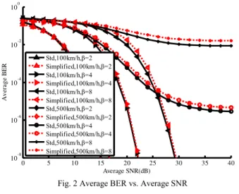
Fig. 2 shows tightness of the simplified average BER approximation for MQAM, according to (12), with different bit rates for velocities 100km/h and 500km/h, respectively. It is evident that the simplified approximation nearly predicts the BER expression given by (11). It also shows that the BER performance degrades with the increase of vehicle speed when the bit rate is fixed. In order to guarantee the BER performance, the bit rate must be reduced under high mobility.

0 5 10 15 20 25 30 35 40 10-8 10-6 10-4 10-2 100 Average SNR(dB) A v er ag e B E R Std,100km/h,β=2 Simplified,100km/h,β=2 Std,100km/h,β=4 Simplified,100km/h,β=4 Std,100km/h,β=8 Simplified,100km/h,β=8 Std,500km/h,β=2 Simplified,500km/h,β=2 Std,500km/h,β=4 Simplified,500km/h,β=4 Std,500km/h,β=8 Simplified,500km/h,β=8

Fig. 2 Average BER vs. Average SNR

IV. ADAPTIVE MQAM/OFDMSCHEME

For adaptive OFDM, different power levels and modulation bit load are allocated to different subchannels. The instantaneous BER of each subchannel is

_ ( [ ]) ( [ ]) 1.6 [ ] ( [ ]) 0.2exp (2 1)( N ICI 1) MQAM k k s k k S BER k P β γ γ γ γ γ ⎡ ₋ ⎤ ⎢ ⎥ ≈ ⎢ ⎥ − + ⎢ ⎥ ⎢ ⎥ ⎣ ⎦ (15) where the transmit signal power ( [ ])s_γ k and ( [ ])_{β γ} k are adapted with [ ]γ k , subject to the average signal power S , and the instantaneous BER constraints BER_MQAM( [ ])_γ k =P_tar .

_

k N ICI

P is the normalized ICI power of the k th subcarrier.

From (6) it follows that

[ ]

(

)

_ , 0, k N ICI k m m m k s k P S γ ρ = ≠ =

∑

(16)

Note that, it is very difficult to calculate the exact

_

Nk ICI

P when the signal powers transmitted over different

subchannels are not the same. However, we can obtain an upper bound for it in terms of the largest transmitted normalized power P_ max max= _m

{

s

(

γ

[ ]

m

)

/S

}

,

[ ]

(

)

1 0 / 1 N m s γ m S − = =

∑

of all the subcarriers easily.

Consequently, employing the upper bound for the normalized

ICI variance of the all subcarriers, determined by _ maxP , the upper bound of the instantaneous BER for each subchannel can be given as _ ( [ ]) ( [ ]) 1.6 [ ] ( [ ]) 0.2exp (2 1)( _max N ICI 1) MQAM _k s k k S BER k P P β γ γ γ γ γ ⎡ ₋ ⎤ ⎢ ⎥ ≤ ⎢ ⎥ − + ⎢ ⎥ ⎢ ⎥ ⎣ ⎦ . (17) According to (17), the maximum bit load size is obtained as

_ 2 ( [ ]) ( 1.6/ ln( / 0.2)) [ ] ( [ ]) log 1 ( _max N ICI 1) tar s k P k S k P P γ γ β γ γ ⎡ ₋ ⎤ ⎢ ⎥ ≤ ⎢ + ⎥ + ⎢ ⎥ ⎢ ⎥ ⎣ ⎦ . (18) The maximum bit load in (18) is a lower bound for each subchannel because of the largest ICI power. According to the assumption A2 for the channel model, it can be shown that the average capacity of an adaptive OFDM system does not depend on the system parameters or on the specific power delay profile of the WSSUS mobile channels [9].

To maximize the average capacity of an adaptive OFDM system, following constrained optimization problem is considered: [ ] ( [ ]) max ( [ ]) _k ( [ ]) [ ] sγ k

∫

β γ k pγ γ k d kγ (19a) subject to [ ]k{ ( [ ])} E_γ sγ k ≤S ∀ ∈k N (19b) ( [ ]) 0 sγ k ≥ ∀ ∈k N (19c) ( [ ]) MQAM tar BER γ k ≤P ∀ ∈k N (19d) where {}E_x ⋅ denotes expectation with respect to x . Then, the Lagrangian for the optimization problem is defined as

_ 2 ( [ ]) ( 1.6 / ln( / 0.2)) [ ] { ( [ ])} log 1 ( _ max N ICI 1) tar s k P k S J s k P P γ γ γ γ ⎡ ₋ ⎤ ⎢ ⎥ = ⎢ + ⎥ + ⎢ ⎥ ⎢ ⎥ ⎣ ⎦

∫

[ ]k ( [ ]) [ ] ( ( [ ]) [ ]k ( [ ]) [ ] ) p_γ γ k d kγ λ sγ k p_γ γ k d kγ S × −

∫

− (20)

where λ is the Lagrange multiplier. The optimal power

adaptation must be nonnegative and satisfy { ( [ ])} 0 ( [ ]) 0 ( [ ]) 0 ( [ ]) J s k s k k s k γ _{γ β γ} γ ∂ _{= ≥ ≥} ∂ ， ， . (21)

Solving (21) yields the optimal power adaptation

_ _ max 1 ( [ ]) 1 ( 1.6 / ln( / 0.2)) [ ] ln(2) N ICI tar P P s k P k S S γ γ γ λ + = − − . (22)

Note that the Lagrange multiplier λ can be determined from the average power constraint using numerical methods. The optimal rate adaptation can then be given as

_ 2 ( 1.6/ ln( / 0.2)) [ ] ( [ ]) log ( ln(2) )( _max N ICI 1) tar P k k S P P γ β γ λ γ ⎡ ₋ ⎤ ⎢ ⎥ = + ⎢ ⎥ ⎣ ⎦ bps/Hz . (23)

In practice, however, only the integer value of the rate is acceptable. Therefore, the rate is truncated to the nearest

integer value. The average capacity of the adaptive OFDM system is then follows as

_ max ₀ 2 ( 1.6 / ln( / 0.2)) [ ] log ( ln(2) )( _ max N ICI 1) tar P k Capacity S P P γ γ λ γ ∞ ⎡_⎢ − ⎤_⎥ = + ⎢ ⎥ ⎣ ⎦

∫

, [ ]k ( [ ]) [ ] p_γ γ k d kγ × (24) where

(

)

( )

(

)

_ 0 _ max 1 ln 2 1.6 / ln / 0.2 N ICI tar P P S P γ λ γ = + − is the optimized

threshold for [ ]γ k below which the channel is not used. Note that, this threshold can be determined from (22) so as to

( [ ]) / 0

s_γ k S≥ . To find the closed-form approximation for (24), we use the pdf of p_{γ[ ]k} ( [ ])γ k given by

[ ]( [ ]) exp( [ ] / [ ]) [ ] k k k p k k γ γ γ γ γ − = . (25)

Here, γ[ ]k =γE H

{ }

_k 2 is the average received SNR and

{ }

2

k

E H is independent of the subcarrier index k , as can be seen from (8), Therefore, [ ]γ k can be substituted by ϕγ . As shown in the Appendix, (24) can be evaluated as

0 max _ln(2)1 Capacity Ei γ ϕγ ⎛ ⎞ = − ⎜− ⎟ ⎝ ⎠ (26) where ( )Ei⋅ denotes the exponential integral [14].

In order to evaluate P_ max in (20), we employ the instantaneous BER expression (15) for each subchannel

k where the normalized ICI power for subchannel is computed.

However, the resulting constraint optimization problem, stated by the Eqs. (19a) to (19b), needs the knowledge of the other subchannel powers, ( [ ]) /sγ m S,m=0,1,"N−1

(

m k≠

)

which makes the solution computationally intractable. One feasible way to solve the problem is to assume that the normalized ICI power of the k th subchannel is determined by its own power. That is, P_{N ICI}k_{_} ≈s( [ ]) /γ m S P× _{N ICI_} . However, the BER performance, in this case, cannot meet the constraint (19d) since the transmit powers of the adjacent subcarriers are larger than that of the k th subcarrier. On the other hand, when H is _k

the best subchannel implies that ( [ ]) /sγ k S as well as P , _ICIk

determined by ( [ ]) /sγ k S , take their maximum values resulting in the constraint (19d) be satisfied. Consequently,

_ max

P can be determined as P_ max lim= _{γ[ ]k−>∞}s( [ ]) /γ k S. We can obtain an upper bound from (22) as

[ ] ( [ ]) 1 _ max lim ( ) ln(2) k s k P S S γ γ λ −>∞ = = (27)

For the worst case, the ICI is determined by the largest power, when [ ]_γ k _{= ∞ and a lower bound on the maximum}

spectral efficiency in adaptive OFDM/MQAM systems is obtained.

V. NUMERICAL RESULTS AND DISCUSSION

In this section, we examine the performance of the solution for the power and rate adaptation derived in the previous sections. In all simulations presented here, we assume =1024N ,

=2.5

c

f GHz, 15_{Δ =}f KHz, v =100km/h and 500km/h. The BER requirement is ₁₀−3_.

In Fig. 3, the adaptive power control scheme ( [ ]) /s_γ k S is plotted as a function of the average SNR. The figure shows similar trends with respect to [ ]_γ k for different velocities. It also indicates that the larger speed yields larger cutoff and larger transmit power as [ ]_γ k _{→ ∞ . The larger cutoff at the}

larger velocities is due to fact that ICI power gets also larger. Higher transmit power at higher speeds as [ ]_γ k _{→ ∞ is also}

due to the average power constraint.

0 10 20 30 40 50 0 0.2 0.4 0.6 0.8 1 1.2 1.4 γ[κ] (dB) s( γ[ κ]) /S 100km/h 500km/h

Fig. 3 s( [ ]) /γ k Sfor MQAM (_{BER=10 , [ ] 35}−3_{γ k = dB)}

0 10 20 30 40 50 0 2 4 6 8 10 12 14 γ[κ] (dB) β( γ[ κ]) 100km/h 500km/h

Fig. 4 β γ( [ ])k for MQAM (_{BER=10 , [ ] 35}−3_{γ k = dB)}

In Fig. 4, the bit rate adaptation ( [ ])β γ k is plotted as a function of the average SNR. We conclude from Fig.4 that it is possible to transmit more bits as [ ]γ k increases and that the larger speed yields the larger cutoff. It also shows that the lower speed has the larger bit rate than higher speed counterpart when [ ]γ k is fixed. As it can be seen from Fig.4, the higher speed case yields lower bit rate than the lower speed case even with larger transmit power because of the larger ICI variance at higher speeds.

Fig. 5 shows the average spectral efficiency of the adaptive OFDM systems as well as of the non-adaptive OFDM for different values of velocities. It also indicates that the higher speeds have lower average spectral efficiency, mainly due to the fact that it induces higher ICI. As it can be seen from Fig.5, the adaptive OFDM can achieve higher gains in spectral efficiency compared with non-adaptive OFDM under different velocities resulting in a floor in the average spectral efficiency. We also observed that the spectral efficiency of the system cannot be improved with the average SNR, increasing beyond a certain level. This is mainly due to the contribution of the average SNR to the ICI. The average spectral efficiencies of truncated integer rate adaptive OFDM are also given in Fig. 5. In spite of the fact that its spectral efficiency is close to the adaptive OFDM, we observe that there is still a certain gap, since the optimal parameters are obtained in the rate-domain.

5 10 15 20 25 30 35 0 1 2 3 4 5 6 7 8 Average SNR (dB) A ver age S pec tr al E ff ic ie ncy( bp s/ H z) Aadaptive,100km/h Truncated adaptive,100km/h Adaptive,500km/h Truncated adaptive,500km/h Non-Adaptive,100km/h Non-Adaptive,500km/h

Fig. 5 Average spectral efficiency vs. Average SNR

VI. CONCLUSIONS

In this paper, a power and rate adaptation scheme has been studied to maximize average spectral efficiency of MQAM/OFDM systems ın the presence of the fast fading channels. Theoretical and numerical results have shown that adaptive OFDM systems under fast fading channels have considerable gain over non-adaptive counterparts. In fact, the proposed adaptive system under fast fading channels tends to have an average floor of spectral efficiency, depending on the ICI and the average SNR. Since very rapidly time varying channels lead to larger ICI, the average spectral efficiency will be seriously degraded under high mobility. Besides, the performance of the truncated integer rate adaptive OFDM was shown to be close to that of the continuous rate adaptive OFDM. Consequently, the truncated version can be applied in practical system for simplicity under high mobility scenarios. APPENDIX A DERIVATION OF (24) _ max ₀ 2 [ ] ( 1.6 / ln( / 0.2)) [ ] log ( ln(2) )( _ max 1) ( [ ]) [ ] N ICI tar up k P k Capacity S P P p k d k γ γ γ λ γ γ γ ∞ ⎡_⎢ − ⎤_⎥ = ⎢ _{⋅ +} ⎥ ⎣ ⎦ ×

∫

Assume ( 1.6 / ln(P_tar/ 0.2)) ξ = − ,η λ=( ln(2) )S ,ψ=( _maxP ⋅PN ICI_ γ+ . 1) max ₀ 2 [ ] 2 0 [ ] log ( [ ]) [ ] 1 [ ] log exp( [ ] / ) [ ] k k Capacity p k d k k k d k γ γ γ ξγ _{γ γ} ηψ ξγ _{γ ϕγ γ} ηψ ϕγ ∞ ∞ ⎡ ⎤ = ⎢ ⎥ ⎣ ⎦ ⎡ ⎤ = ⎢ ⎥⋅ − ⎣ ⎦

∫

∫

For t=γ[ ]k − , we can express the above integral as follows γ₀ 0 max ₀ 0 ( ) 1 _{ln exp( ( ) / )} ln(2) t Capacity ξ γ t _{γ ϕγ} dt ηψ ϕγ ∞ ⎡ + ⎤ = ⎢ ⎥ − + ⎣ ⎦

∫

By means of the integral formula 0 1 ln( t 1) exp( ut) exp( ) (u Ei u) u χ χ χ ∞ + − = − −

∫

we obtain the final result as follows

( )

0 max _{ln 2}1 Capacity Ei γ ϕγ ⎛ ⎞ = − ⎜− ⎟ ⎝ ⎠ (28)

REFERENCES

[1] R. Prasad, OFDM for wireless communications systems. Artech House Publishers, 2004.

[2] H. C. Wu, “Analysis and characterization of intercarrier and interblock interferences for wireless mobile OFDM systems,” IEEE Trans.

Broadcasting, vol. 52, no. 2, pp. 203-210, Jun. 2006.

[3] L. Ong, M. Shikh-Bahaei, and J. A. Chambers, “Variable rate and variable power MQAM system based on Bayesian bit error rate and channel estimation techniques,” IEEE Trans. Commun., vol. 56, no. 2, pp. 177–182, Feb. 2008.

[4] C. Liu, D. Bielefeld, and R. Mathar, “Optimal rate and power allocation for OFDM in the presence of channel uncertainty,” in Proc. IEEE PIMRC, pp. 1–5, Sep. 2008.

[5] Z. Mao and X. Wang, “Efficient optimal and suboptimal radio resource allocation in OFDMA system,” IEEE Trans. Wireless Commun., vol.7, no. 2, pp. 440–445, Feb. 2008.

[6] J. Huang, V. G. Subramanian, R. Agrawal, and R. A. Berry, “Downlink scheduling and resource allocation for OFDM systems,” IEEE Trans.

Wireless Commun., vol. 8, no. 1, pp. 288–296, Jan. 2009.

[7] H. Cheon and D. Hong, “Effect of channel estimation error in OFDM-based WLAN,” IEEE Commun. Lett., vol. 6, no. 5, pp. 190–192, May 2002. [8] L. Rugini and P. Banelli, “BER of OFDM systems impaired by carrier frequency offset in multipath fading channels,” IEEE Trans. Wireless

Commun., vol. 4, no. 5, pp. 2279–2288, Sep. 2005.

[9] K. Nehra and M. Shikh-Bahaei, “Spectral efficiency of adaptive mqam/ofdm systems with CFO over fading channels”, IEEE Trans. Veh.

Techn., vol. 60, no. 3, pp. 1240–1246, Mar. 2011.

[10] Y.-S. Choi, P. J. Voltz, and F. A. Cassara, “On channel estimation and detection for multicarrier signals in fast and selective Rayleigh fading channels,” IEEE Trans. Commun., vol. 49, no.8, pp. 1375-1387, Aug. 2001. [11] X. Cai, and G. B. Giannakis, “Bounding performance and suppressing intercarrier interference in wireless mobile OFDM,” IEEE Trans.

Commun., vol. 51, no. 12, pp. 2047-2056, Dec. 2003.

[12] S. Ye, R. S. Blum, and L. J. Cimini, “Adaptive OFDM systems with imperfect channel state information,” IEEE Trans. Wireless Commun., vol. 5, no. 11, pp. 3255–3265, Nov. 2006.

[13] S. T. Chung, and A. J. Goldsmith, “Degrees of freedom in adaptive modulation: a unified view,” IEEE Trans. Commun., vol. 49, no. 9, pp. 1561-1571, Sep. 2001.

[14] I. S. Gradshteyn and I. M. Ryzhik, Table of Integrals, Series, and Products,