A NEW APPROACH TO AGE AND RISK
TAKING BEHAVIOR OF AGENTS
A Master’s Thesis
by
Zeynep KOZAN
Department of
Economics
·
Ihsan Do¼
gramac¬Bilkent University
Ankara
A NEW APPROACH TO AGE AND RISK TAKING BEHAVIOR
OF AGENTS
Graduate School of Economics and Social Sciences
of
·
Ihsan Do¼
gramac¬Bilkent University
by
ZEYNEP KOZAN
In Partial Ful…llment of the Requirements For the Degree
of
MASTER OF ARTS
in
THE DEPARTMENT OF ECONOMICS ·IHSAN DO ¼GRAMACI BILKENT UNIVERSITY ANKARA
I certify that I have read this thesis and have found that it is fully adequate, in scope and in quality, as a thesis for the degree of Master of Arts in Economics.
— — — — — — — — — — — — — — — — — — – Assist. Prof. Dr. Emin Karagözo¼glu Supervisor
I certify that I have read this thesis and have found that it is fully adequate, in scope and in quality, as a thesis for the degree of Master of Arts in Economics.
— — — — — — — — — — — — — — — — — – Assist. Prof. Dr. Tar¬k Kara
Examining Committee Member
I certify that I have read this thesis and have found that it is fully adequate, in scope and in quality, as a thesis for the degree of Master of Arts in Economics.
— — — — — — — — — — — — — — Assoc. Prof. Dr. Hüseyin Merdan Examining Committee Member
Approval of the Graduate School of Economics and Social Sciences
— — — — — — — — — Prof. Dr. Erdal Erel Director
ABSTRACT
A NEW APPROACH TO AGE AND RISK TAKING
BEHAVIOR OF AGENTS
KOZAN, Zeynep
M.A., Department of Economics
Supervisor: Assist. Prof. Dr. Emin Karagözo¼glu September 2012
In this thesis, we use evolutionary game theory techniques to analyze the rela-tion between risk taking behavior of agents and their ages. We suppose that risk aversion is the stable pattern for the old agents and risk seeking is the stable pattern for the young agents as it is commonly assumed so in economics literature. First, we solve a benchmark model without heterogeneity in terms of age di¤erentiations. In such a case, we observe that mutation either increases or decreases with respect to the payo¤ levels, depending on the initial …tness levels of the population groups. In the second step, we introduce heterogeneous pop-ulation frontier. The anticipated level of the initial mutant proportion provides incentives to triger the evolution. Then, we analyze numerically the e¤ects of the initial level of …tness, initial risk averse and risk seeking proportions on the pattern of the evolution process. Finally, we studied the intertemporal e¤ects of di¤erent risk averse and risk seeking population proportions on mutation.
Keywords: Risk Aversion, Risk Seeking, Risk Dominant Equilibrium, Evolu-tionary Game Theory, Age and Risk, Coordination Games
ÖZET
YA¸
S VE B·
IREYLER·
IN R·
ISK ALMA
DAVRANI¸
SLARINA YEN·
I B·
IR YAKLA¸
SIM
KOZAN, Zeynep
Yüksek Lisans, Ekonomi Bölümü
Tez Yöneticisi: Assist. Prof. Dr. Emin Karagözo¼glu Eylül 2012
Bu tezde, bireylerin risk alma davran¬¸slar¬ile ya¸slar¬aras¬ndaki ili¸skiyi analiz et-mek için evrimsel oyun teorisi tekniklerini kullan¬yoruz. Ekonomi literatüründe kabul edildi¼gi üzere riskten kaç¬nman¬n ya¸sl¬lar için, risk aray¬¸s¬n¬n ise gençler için dura¼gan davran¬¸s biçimi oldu¼gunu varsay¬yoruz. Öncelikle, ya¸s farkl¬la¸ smas¬kap-sam¬nda heterojenlik içermeyen temel bir model çözüyoruz. Böyle bir durumda, popülasyon gruplar¬n¬n ba¸slang¬ç uyum seviyeleri durumuna ba¼gl¬olarak mutasy-onun kazanç seviyelerine göre artt¬¼g¬n¬ya da azald¬¼g¬n¬gözlemliyoruz. ·Ikinci a¸ sa-mada, modele popülasyon heterojenli¼gi ekliyoruz. Böyle bir modelde, öngörülen ba¸slang¬ç mutant oranlar¬, evrimin tetiklenmesini sa¼gl¬yor. Daha sonra, ba¸slang¬ç uyum seviyesinin, ba¸slang¬ç riskten kaç¬nma ve ba¸slang¬ç risk aray¬¸s¬oranlar¬n¬n, evrim sürecine etkilerini nümerik olarak inceliyoruz. Son olarak, popülasyondaki farkl¬ riskten kaç¬nma ve risk aray¬¸s¬ oranlar¬n¬n mutasyon üzerindeki zaman-lararas¬etkilerini ara¸st¬r¬yoruz.
Anahtar Kelimeler: Risten Kaç¬nma, Risk Aray¬¸s¬, Risk Bask¬n Denge, Evrimsel Oyun Teorisi, Ya¸s ve Risk, Kordinasyon Oyunlar¬
ACKNOWLEDGEMENTS
I would like to express my deepest gratitude to my supervisor, Assist. Prof. Emin Karagözo¼glu, who has supported me throughout my thesis with his pa-tience, knowledge and exceptional guidance in all of the stages of my study. I am indebted to him. I would like to thank Assist. Prof. Tar¬k Kara, as one of my thesis examining committee members, who gave his time and provided wor-thy guidance. I also would like to thank Assoc. Prof. Hüseyin Merdan for his interest and helpful suggestions as an examining committee member and for his great support throughout my academic life.
Thanks to Bilkent University for its …nancial support during my graduate study.
Special thanks to my undergraduate professors, who have always been there and continued on giving me the moral support during my graduate study.
I would like to thank my family for being always there with all their love and continuous support, during my graduate study and entire life.
However, while grateful to them, I bear the sole responsibilities for all the mistakes made in the thesis.
TABLE OF CONTENTS
ABSTRACT . . . iii
ÖZET . . . iv
ACKNOWLEDGMENTS . . . v
TABLE OF CONTENTS . . . vi
LIST OF TABLES . . . vii
LIST OF FIGURES . . . viii
CHAPTER 1: INTRODUCTION . . . .1
CHAPTER 2: THE BENCHMARK MODEL . . . 5
2.1 The Evolutionary Game. . . 5
2.1.1 The Young Agents . . . 8
2.1.2 The Old Agents . . . 10
2.1.3 Heterogeneity . . . 11 2.1.3.1.1 Case. . . .. . . 17 2.1.3.1.2 Case. . . .. . . 18 2.1.3.1.3 Case. . . .. . . 18 2.1.3.2.1 Case. . . .. . . .. . . 21 2.1.3.2.2 Case. . . .. . . .. . . 21 2.1.3.3.3 Case. . . .. . . 21
CHAPTER 3: NUMERICAL ANALYSIS . . . 24
CHAPTER 4: CONCLUSION . . . 30
LIST OF TABLES
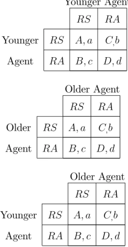
1. General payo¤ tables of the model . . . .. . . .7
2. Two player game between young agents . . . .. . . .10
3. Two player game between old agents. . . .. . . .11
4. Two player game between young and old agents . . . .... . . .13
5. The values of the di¤erence between the average …tness of the risk aversion of young population and the average …tness of the entire population for di¤erent proportion levels of risk averse youngs and risk averse olds . . . . .. . . .22
6. The values of the di¤erence between the average …tness of the risk aversion of young population and the average …tness of the entire population for di¤erent proportion levels of risk averse youngs and only risk seeking olds, qra = 0 or only risk averse olds, qra = 1 . . . .. . . .24
7. Intertemporal analysis of risk dominant strategy frequency and payo¤ domi-nant strategy frequency permanence for di¤erent scenarios . . . 25
LIST OF FIGURES
1. Average Fitness of Risk Averse Youngs . . . .. . . 20 2. Average Fitness of Risk Seeking Olds . . . 23
CHAPTER 1
INTRODUCTION
There are numerous studies in economics literature which studied the e¤ect of age on risk-taking. These studies show that, the well-known conclusion, risk taking de-creases with age (Morin and Suarez, 1983; Holmstrom and Milagrom, 1987; Kanodia et al., 1989; Riley and Chow, 1992). Using di¤erent measures such as observed port-folio allocations of wealth (Jianakoplos and Bernasek, 2006) or large scale survey studies analyzing the whole population (Barsky et al., 1997; Donkers et al., 2001; Dohmen et al., 2006), these studies show that willingness to take risk is decreasing with age. Using the lowa Gambling Task, a task to measure ambiguity, various stud-ies also …nd a negative correlation between risk taking and age (Fein et al., 2007; Denburg et al., 2005; Zamarin et al., 2008). Further studies found that violations of expected utility theory are decreasing with age (Kume and Suzuki, 2010; Harbaugh et al., 2002).
On the other hand there are various studies in psychology literature which show that older adults may be more risk seeking than younger adults. Considering the framing e¤ects on young and old agents they conclude that old agents are more likely to be risk averse (i.e., to move away from a risky option) when questions are framed as gains (i.e., positively) and more risk seeking (i.e., to move toward a risky option) when questions are framed as losses (i.e., negatively), (Hasher et al., 2005; Lauriola and Levin, 2001). By considering such a psychological result, our motivation is that
under negative conditions such as the last …nancial crises the world experienced, could the old agents evaluate these conditions as a negative frame? For instance, also Weber at al. (2004) did a meta analysis of studies involving decision outcomes described to study participants and found that increasing age (age ranges were not speci…ed in their paper) was associated with greater risk seeking (more choices of a gamble over a sure thing) in losses; they did not, however, …nd a link between increasing age and risk aversion (more choices of a sure thing over a gamble) in gains. Another study which was presented by Arkes and Ayton (1999), displays an empirical evidence from studies on sunk-cost e¤ects. There is an interesting di¤erence in test results between adults and children with regard to the sunk-cost e¤ect. Children under 10 years of age seem to be less susceptible to the sunk-cost e¤ect than humans of older ages. Arkes and Ayton explain this by the fact that young humans have more modest cognitive abilities. These cognitive abilities are suggested to be the main explanation for sunk-cost e¤ects, because humans, especially adults, tend to de…ne complex strategies (Janssen and Sche¤er, 2004).
A contrary to the well-known results (i.e., risk aversion increases with age) in economics is Wang and Hanna’s (1997) research which is consistent with the results in psychology literature we mentioned above. Using the 1983-1989 panel of the survey of consumer …nances they …nd out that relative risk aversion decreases as people age (i.e., the proportion of net wealth invested in risky assets increases as people age). They show that risk tolerance increases with age which is contrary to constant life-cycle risk aversion hypothesis. Their conclusion is young people may appear more risk averse since it is hard for them to endure any short-term investment losses with limited …nancial resources. Future human wealth cannot be applied to pay present bills, car loans, mortgage debts, etc. Besides, William B. Riley Jr. and K. Victor Chow (1992), who studied asset allocation and individual risk aversion in their research, showed that risk aversion decreases with age- but only up to a point. After age 65 (retirement), risk aversion increases with age.
to age is extended by using insight from research on human decision making. Al-though the common belief in economics lays out that the old humans are more risk averse, while the young ones are more risk seeking, “why” there does not exist coherence with the studies in psychology literature. There is no any research in the literature which tries to present an explanation to this mismatching we observe in these two di¤erent disciplines. This is the main motivation for this research to be able to introduce a link between both disciplines and discard this dualism by a theoretical model. One of the questions we address is “why” humans of older ages may invest on risky options while the humans of young ages are not subject to invest on them. In our view, an important factor that might explain these is the “sunk-cost e¤ect”— where human decision making is typically in‡uenced by the level of prior investments. Janssen and Sche¤er (2004:6) claim that "According to conventional economic theory, only the incremental costs and bene…ts of the current options should be included in decision making. However, numerous examples show that humans do take into account prior investment when they consider what course of action to follow." Hence, the learning procedure of agents will be an important input in our work to study the analysis of repositioning of them according to their risk attitudes under evolutionary dynamics.
We will form a model as an evolutionary game which examines the feasible strategies that is known in the literature (old people are more risk-averse than young ones) versus the deviation from these strategies (old can choose to act in a more risk seeking manner). At this point, we will consider the risk aversion as the stable pattern of behavior among the older agents and risk seeking is stable among the younger ones in a population, since the common belief is so in economics literature. In other words, the literature supposes that the agents are programmed to play particular strategies. Such an assumption supports that a stable pattern of behavior in a population should be able to eliminate any invasion by a “mutant”, and to do so it must have a higher …tness than the mutant in the population that results from the invasion. Here, the payo¤ of an agent by playing a particular strategy
is interpreted as “…tness”. By introducing two equilibrium into the model which are constituted by payo¤ dominant and risk dominant strategies set, the deviations between these strategies are possible to be examined.
Finally, we will use “replicator dynamics” as the evolutionary dynamic, which are …rst called by Taylor and Jonker (1978) and Zeeman (1979), to investigate the dynamic properties of an evolutionary stable strategy (ESS). This dynamic speci…es that the proportional rate of growth in a strategy’s representation in the population, p, is given by the extent to which that strategy does better than the population average.
The main perspective of this work is taking agents as heterogeneous among their life-cycles. For this issue we will work on their decision taking processes by investi-gating the results of such a heterogeneity. By using evolutionary game framework, one of the main purposes of the model is to …nd the proportions of risk aversion and risk seeking among di¤erent populations at which level they work as a threshold for evolution. There exists limited number of studies focused on what population aging would mean for economic decisions that are sensitive to risk taking characteristics of a population. Then, the solidity of the models used in economics, which have left such a possible behavioral diversi…cation among agents out of account, should be questioned. In this thesis, we question in spite of the fact that there exist some researches about the risk taking behavior of agents and how it changes among them with respect to their ages, why such a new approach is not used in existing models. The organization of the paper is as follows. In Chapter 2, the benchmark model will be introduced and solved by using evolutionary game which is constituted by both a risk dominant equilibrium and a payo¤ dominant equilibrium. Since the games we introduced for youngs and olds are symmetric games, we will present the results for youngs without loss of generality. In Chapter 3, numerical analysis and comparative statics for the parameters of the game will take place. Finally, Chapter 4 concludes the paper.
CHAPTER 2
THE BENCHMARK MODEL
2.1
The Evolutionary Game
In this section we construct an explicit model of the process by which the frequency of strategies changes in the population and study properties of the evolutionary dynamics within the model. Thus, once the model of the population dynamics has been speci…ed, all of the standard stability concepts used in the analysis of dynamical system can be brought to bear.
In this research, each game is played between (and among) the young and older agents. Recalling the Riley and Chow’s framework, older agents will be taken as the ones under the age of 65, and the ones above are excepted as retired. We will examine each game, which are played by only youngs, played by only olds, and …nally played between youngs and olds, in detail section by section.
The basic model is of a repeated game played in periods t = 1; 2; 3; :::.The population is large enough. In each period, individuals choose one of two possible actions, “Risk Aversion” and “Risk Seeking” which are denoted by RA and RS. That is ait 2 fRA; RSg. Formally, it is required that A > B and D > C so that
(RS; RS) and (RA; RA) are both Nash equilibria. In addition, we assume that (D C) (A B)for the younger agents so that (RA; RA) is the "risk dominant" equilibrium. Since the economics literature claims that risk seeking is more common among the young agents, it is consistent with Harsanyi and Selten (1988) taking the
strategy set (RS; RS) as payo¤ dominant for the young individuals. Note that when the strategies have equal security levels (B = C), (RA; RA) is also the Pareto optimum. Similarly, (RS; RS) will be the "risk dominant" equilibrium for the game which is played by old agents. Hence, we will assume that A > B and D > C for that game. In addition, we will assume that (A B) > (D C) for the olds, and when (B = C), (RS; RS) will also be Pareto optimum of that game.
Table 1. General payo¤ tables of the model Younger Agent RS RA Younger RS A; a C;b Agent RA B; c D; d Older Agent RS RA Older RS A; a C;b Agent RA B; c D; d Older Agent RS RA Younger RS A; a C;b Agent RA B; c D; d
How a population in which these plays are repeatedly played will evolve in terms of its risk taking characteristics is the main question. First, assume that the pop-ulation is quite large. In this case, we can represent the state of the poppop-ulation by simply keeping track of what proportion follows the strategies RA and RS. Let pra
and prs (without loss of generality, qra and qrs for the old population) denote these
proportions. Furthermore, let the average …tness of risk aversion and risk seeking be denoted by WRA and WRS, respectively, and let W be the average …tness of the
entire population. The values of WRA, WRS, and W can be expressed in terms of
WRA = F0+ pra F (RA; RA) + prs F (RA; RS); (1)
WRS = F0+ pra F (RS; RA) + prs F (RS; RS); (2)
W = praWRA+ prsWRS: (3)
Second, let us assume that the proportion of the population following the strate-gies RA and RS in the next generation is related to the proportion of the population following the strategies RA and RS in the current generation according to the rule:
p0ra = praWRA
W ; (4)
p0rs = prsWRS
W : (5)
We can rewrite these expressions in the following form:
p0ra pra = pra(WRA W ) W ; (6) p0rs prs = prs(WRS W ) W : (7)
If we assume that the change in the strategy frequency from one generation to the next are small, then the replicator dynamics:
dpra dt = pra(WRA W ) W ; (8) dprs dt = prs(WRS W ) W : (9)
The replicator dynamics may be used to model a population of individuals play-ing the game we introduced above. For this game, the expected …tness of “Risk
aversion” and “Risk seeking” are expressed as follows:
WRA = F0+ pra F (RA; RA) + prs F (RA; RS) (10)
= F0+ praD + prsB (11)
and
WRS = F0+ pra F (RS; RA) + prs F (RS; RS) (12)
= F0+ praC + prsA (13)
By looking at the values of utility levels, we will analyze whether the following indicators are positive or not:
WRS W
W (14)
and
WRA W
W : (15)
If an action ai taken by some individuals does better than average, its
represen-tation in the population grows (dpai=dt > 0), and if another strategy is even better,
then its growth rate is also higher than that of strategy ai.
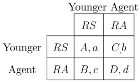
The payo¤ matrix of the game which is played between young agents can be taken as follows:
Table 2. Two player game between young agents Younger Agent
RS RA
Younger RS A; a C;b
Agent RA B; c D; d
where the equilibrium (RS; RS) is Pareto dominant and the equilibrium (RA; RA) is risk dominant. Then,
WRA = F0+ praD + prsB; (16) WRS = F0+ praC + prsA; (17) W = praWRA+ prsWRS: (18) Hence, WRA W W = F0+ praD + prsB pra(F0+ praD + prsB) prs(F0 + praC + prsA) praWRA+ prsWRS = F0+ praD + prsB praF0 p 2 raD praprsB prsF0 prspraC p2rsA praWRA+ prsWRS = (1 pra prs)F0 + (pra p 2 ra)D + (prs praprs)B prspraC p2rsA praF0+ p2raD + praprsB + prsF0+ prspraC + p2rsA = (pra p 2 ra)D + prs praprs)B prspraC p2rsA F0+ p2raD + praprsB + prspraC + p2rsA = pra(1 pra)D + prs(1 pra)B prspraC p 2 rsA F0+ p2raD + praprsB + prspraC + p2rsA = (praD + prsB)(1 pra) prs(praC + prsA) F0+ p2raD + praprsB + prspraC + p2rsA = prs[praD + prsB praC prsA] F0+ p2raD + praprsB + prspraC + p2rsA = prs[pra(D C) + prs(B A)] F0+ p2raD + praprsB + prspraC + p2rsA :
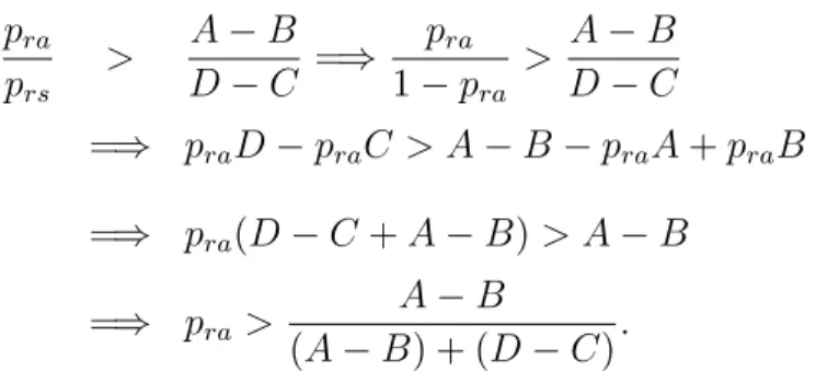
Therefore, since prs > 0; pra> 0; and D > C; if pra(D C) > prs(A B); then WRA W
W > 0: Thus, the representation of the action RA in the young population
grows. That is, if the following condition for the proportion of mutants in the young population is satis…ed, then we expect a rise in the representation of the mutant strategy among the young agents:
pra prs > A B D C =) pra 1 pra > A B D C =) praD praC > A B praA + praB =) pra(D C + A B) > A B =) pra > A B (A B) + (D C):
This result is consistent with Kandori, Mailath, and Rob (1993) and Ellison (1993) who studied the dynamics of a model constituted by a 2x2 coordination game with uniform matching.
2.1.2 The Old Agents
The payo¤ matrix of the game which is played between young agents can be taken as follows:
Table 3. Two player game between old agents Older Agent
RS RA
Older RS A; a C;b
Agent RA B; c D; d
where the equilibrium (RA; RA) is Pareto dominant and the equilibrium (RS; RS) is risk dominant. Then,
WRA = F0+ qraD + qrsB; (19)
WRS = F0+ qraC + qrsA; (20)
W = qraWRA+ qrsWRS: (21)
Therefore, since qrs > 0; qra > 0; and A > B; if qrs(A B) > qra(D C); then WRS W
W > 0: Thus, the representation of the action RS in the old population grows.
That is, whenever the following condition as of the mutants’proportion in the old population is satis…ed, we expect a rise in the representation of the mutant strategy among the old agents:
qrs qra > D C A B =) qrs 1 qrs > D C A B =) qrsA qrsB > D C qrsD + qrsC =) qrs(A B + D C) > D C =) qrs> D C (D C) + (A B): 2.1.3 Heterogeneity
In a large population it is reasonable to assume that population is constituted by di¤erent kinds of agents belonging to various age groups. Here we suggest that this di¤erence among the agents creates a kind of heterogeneity in the population. Hence, it is necessary probing into a case of matching process of players as of di¤erent age groups.
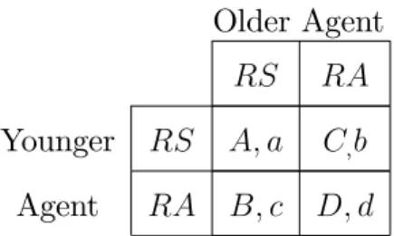
The payo¤ matrix of the game which is played between young agents and old agents can be taken as follows:
Table 4. Two player game between young and old agents Older Agent
RS RA
Younger RS A; a C;b
Agent RA B; c D; d
Assume that the population size is N: Let the number of the youngs as of this population be n, hence the number of olds will be N n: Thus, (pRAyoung)n gives
the share of the risk averse youngs and (pRSyoung)ngives the share of the risk seeking
youngs in the population. Similarly, pRAold(N n) gives the share of the risk averse
olds and pRSold(N n) gives the share of the risk seeking olds in the population.
The probability of matching of a young with an old can be taken as N n N 1 = :
Then, the probability of matching of a young with another young agent will be
n 1
N 1 = 1 :
Therefore, the average …tness for the young population can be written as follows:
WRA = F0+ (pRAyoungD + pRSyoungB) (1 ) + [F0+ (pRAoldD + pRSoldB)] :
WRS = F0+ (pRAyoungC + pRSyoungA) (1 ) + [F0+ (pRAoldC + pRSoldA)] :
Let pRAyoung = pra and pRSyoung = prs for a simplier notation. Similarly, let
pRAold = qra and pRSold = qrs: Then the average …tness of the whole population is
obtained as follows:
W = praqraWRA+ prsqrsWRS:
WRA W W = (F0+ praD + prsB)(1 ) + (F0 + qraD + qrsB) praqraWRA+ prsqrsWRS praqra[(F0+ praD + prsB)(1 ) + (F0+ qraD + qrsB) ] praqraWRA+ prsqrsWRS prsqrs[(F0+ praC + prsA)(1 ) + (F0+ qraC + qrsA) ] praqraWRA+ prsqrsWRS : WRA W W = (1 )F0+ F0 (1 )praqraF0 (1 )prsqrsF0 praqraWRA+ prsqrsWRS praqraF0+ prsqrsF0 praqraWRA+ prsqrsWRS +(1 )(praD + prsB) (1 )praqra(praD + prsB) praqraWRA+ prsqrsWRS + (qraD + qrsB) praqra(qraD + qrsB) praqraWRA+ prsqrsWRS (1 )prsqrs(praC + prsA) prsqrs(qraC + qrsA) praqraWRA+ prsqrsWRS : Finally we have WRA W W = [pra(1 qra) + qra(1 pra)] F0 praqraWRA+ prsqrsWRS +(1 pra)(1 qra)[( 1)(1 pra) (1 qra)] praqraWRA+ prsqrsWRS A +[(1 )(1 pra) + (1 qra)] (1 praqra) praqraWRA+ prsqrsWRS B +(1 pra)(1 qra) [( 1)pra qra] praqraWRA+ prsqrsWRS C +[(1 )pra+ qra] (1 praqra) praqraWRA+ prsqrsWRS D:
Since praqraWRA + prsqrsWRS > 0; it is su¢ cient to investigate whether the
WRA W = [pra(1 qra) + qra(1 pra)] F0 +(1 pra)(1 qra)[( 1)(1 pra) (1 qra)]A +(1 praqra) [(1 )(1 pra) + (1 qra)] B +(1 pra)(1 qra) [( 1)pra qra] C +(1 praqra) [(1 )pra+ qra] D > 0:
The equality above also enable us to examine the necessary conditions for related payo¤s to observe an increase in mutation behavior in a population.1 That is to
say that for a given population, by determining the proper payo¤ levels which are presented to the agents, a population can be directed to a particular behavior. Con-sequently, when the inequalities below hold, this guarantees that the risk dominant strategy, RA; will dominate the young population:
A > pra(qra 1) + qra(pra 1) (pra 1)(qra 1)(pra pra+ qra 1) F0 (praqra 1)(pra 1) (pra qra)(praqra 1) (pra 1)(qra 1)(pra pra+ qra 1) B (pra 1)(qra 1)(pra pra+ qra) (pra 1)(qra 1)(pra pra+ qra 1) C pra+ (pra qra)(praqra 1) (pra 1)(qra 1)(pra pra+ qra 1) D
1The mathematical computing program cannot enable us to solve for the payo¤ level D
B > pra(qra 1) + qra(pra 1) (praqra 1)(pra 1) (pra qra)(praqra 1) F0 (pra 1)(qra 1)(pra pra+ qra 1) (praqra 1)(pra 1) (pra qra)(praqra 1) A (pra 1)(qra 1)(pra pra+ qra) (praqra 1)(pra 1) (pra qra)(praqra 1) C pra+ (pra qra)(praqra 1) (praqra 1)(pra 1) (pra qra)(praqra 1) D C > pra(qra 1) + qra(pra 1) (pra 1)(qra 1)(pra pra+ qra) F0 +(pra 1)(qra 1)(pra pra+ qra 1) (pra 1)(qra 1)(pra pra+ qra) A +(praqra 1)(pra 1) (pra qra)(praqra 1) (pra 1)(qra 1)(pra pra+ qra) B + pra+ (pra qra)(praqra 1) (pra 1)(qra 1)(pra pra+ qra) D
Similarly, for a given population and given game, under particular payo¤ levels if the condition below holds for the initial …tness of the young population, it is guaranteed that an increase in mutation among the young agents will be observed:
F0 > (pra 1)(qra 1)(pra pra+ qra 1) pra(qra 1) + qra(pra 1) A +(praqra 1)(pra 1) (pra qra)(praqra 1) pra(qra 1) + qra(pra 1) B (pra 1)(qra 1)(pra pra+ qra) pra(qra 1) + qra(pra 1) C +pra+ (pra qra)(praqra 1) pra(qra 1) + qra(pra 1) D
Similarly, the probability of matching of an old with a young can be taken as
n
N 1 = 1 + , where =
1
N 1:Then, the probability of matching of an old with
old agents, the average …tness for the old population can be written as follows:
WRA = F0 + (pRAyoungD + pRSyoungB) (1 + ) + [F0 + (pRAoldD + pRSoldB)] ( )
WRS = F0 + (pRAyoungC + pRSyoungA) (1 + ) + [F0+ (pRAoldC + pRSoldA)] ( )
and W = praqraWRA+ prsqrsWRS: Therefore, WRS W W = (F0+ praC + prsA)(1 + ) + (F0+ qraC + qrsA)( ) praqraWRA+ prsqrsWRS praqra[(F0+ praD + prsB)(1 + ) + (F0 + qraD + qrsB)( )] praqraWRA+ prsqrsWRS prsqrs[(F0+ praC + prsA)(1 + ) + (F0 + qraC + qrsA)( )] praqraWRA+ prsqrsWRS : WRS W W = (1 + )F0 (1 + )praqraF0 (1 + )prsqrsF0 praqraWRA+ prsqrsWRS +( )F0 ( )praqraF0 ( )prsqrsF0 praqraWRA+ prsqrsWRS +(1 + )(praC + prsA) (1 + )prsqrs(praC + prsA) praqraWRA+ prsqrsWRS +( )(qraC + qrsA) ( )prsqrs(qraC + qrsA) praqraWRA+ prsqrsWRS (1 + )praqra(praD + prsB) + ( )praqra(qraD + qrsB) praqraWRA+ prsqrsWRS : Finally we have
WRS W W = [(1 prs)qrs+ (1 qrs)prs] F0 praqraWRA+ prsqrsWRS +[(1 + )prs+ ( )qrs] (1 prsqrs) praqraWRA+ prsqrsWRS A +(1 prs)(1 qrs) [( 1 )prs ( )qrs] praqraWRA+ prsqrsWRS B +[(1 + )(1 prs) + ( )(1 qrs)] (1 prsqrs) praqraWRA+ prsqrsWRS C +(1 prs)(1 qrs)[( 1 )(1 prs) ( )(1 qrs)] praqraWRA+ prsqrsWRS D:
Hence, if the condition below holds, then the mutant strategy risk seeking, RS; will dominate the old population:
WRS W = [(1 prs)qrs+ (1 qrs)prs] F0 +(1 prsqrs) [(1 + )prs+ ( )qrs] A +(1 prs)(1 qrs) [( 1 )prs ( )qrs] B +(1 prsqrs) [(1 + )(1 prs) + ( )(1 qrs)] C +(1 prs)(1 qrs)[( 1 )(1 prs) ( )(1 qrs)]D > 0: Case 2.1.3.1.1: pra = qra = 1; WRA W = 0:
Conclusion 1 If there exist only risk averse olds and risk averse youngs in a pop-ulation, then any representation of the mutant strategy among the youngs will not be observed.
Case 2.1.3.1.2: pra 2 [0; 1] and qra = 1;
WRA W = (1 pra)F0+ (1 )(1 pra)2B + [(1 )pra+ ] (1 pra)D > 0:
Conclusion 2 If there exist only risk averse old agents in a population, then the representation of the action RA in the young population grows. That is to say that the representation of the mutant strategy among the youngs arises.
Case 2.1.3.1.3: pra 2 [0; 1] and qra = 0;
WRA W = praF0+ (1 pra)[( 1)(1 pra) ]A
+[(1 )(1 pra) + ]B
+(1 pra)[( 1)pra qra]C
Case 2.1.3.2.1: prs = qrs = 1;
WRS W = 0:
Conclusion 3 If there exist only risk seeking youngs and risk seeking olds in a population, then any representation of the mutant strategy among the olds will not be observed.
Case 2.1.3.2.2: qrs 2 [0; 1] and prs = 1;
WRS W = (1 qrs)F0+ (1 qrs)( )qrsA + (1 qrs)2( )C > 0:
Conclusion 4 If there exist only risk seeking young agents in a population, then the representation of the action RS in the old population grows. That is to say that the representation of the mutant strategy among the olds arises.
Case 2.1.3.2.3: qrs 2 [0; 1] and prs = 0;
WRS W = qrsF0+ ( )qrsA
( )(1 qrs)qrsB
+[(1 + ) + ( )(1 qrs)]C
CHAPTER 3
NUMERICAL ANALYSIS
In this section, we perform the numerical analysis and comparative statics. We examine how risk aversion will roll among the young agents for some sample values of initial proportions of the risk averse youngs and risk averse olds for the game which is played between youngs and olds. Under heterogeneity, we present the mutation behavior among the youngs as of raise and fall tendency and the …nal circumstance of the mutant invasion. Thus, we are able to obtain the necessary proportion conditions of the agent groups playing the mutant strategy to observe an increase in mutation, thus an invasion of the entire population. That is, we analyze how the …tness of risk aversion of young people position itself in di¤erent heterogeneous agent groups.
Without loss of generality in this section we will make our analsis for some reasonable sample values for the payo¤s of each game such that A = 5, B = 4, C = 0, and D = 2. These payo¤s are consistent with our assumption that each game has one payo¤ dominant equilibrium and one risk dominant equilibrium.
Moreover, we also make our analysis for di¤erent initial …tness levels, F0, which
work as initial endowment for the agents in the economy. Hence, the results we found by encoding di¤erent levels of F0 into the model will be an important indicator of
analyzing the mutation behavior.
Table 5. The values of the di¤erence between the average …tness of the risk aversion of young population and the average …tness of the entire population for
di¤erent proportion levels of risk averse youngs and risk averse olds when F0 = 1; 5; 10; 50; 0; 1; 3; 4respectively ( = 0:5) pra qra WRA W WRA W WRA W WRA W 0:00 0:00 1:000 1:000 1:000 1:000 0:05 0:05 0:301 0:078 0:553 4:353 0:10 0:10 0:297 1:017 1:917 9:117 0:15 0:15 0:801 1:821 3:096 13:30 0:20 0:20 1:216 2:496 4:096 16:90 0:25 0:25 1:547 3:047 4:922 19:92 0:30 0:30 1:799 3:479 5:579 22:38 0:35 0:35 1:978 3:798 6:073 24:27 0:40 0:40 2:088 4:008 6:408 25:61 0:45 0:45 2:135 4:115 6:590 26:39 0:50 0:50 2:125 4:125 6:625 26:63 0:55 0:55 2:062 4:042 6:517 26:32 0:60 0:60 1:952 3:872 6:272 25:47 0:65 0:65 1:800 3:620 5:895 24:09 0:70 0:70 1:611 3:291 5:391 22:19 0:75 0:75 1:391 2:891 4:766 19:77 0:80 0:80 1:144 2:424 4:024 16:82 0:85 0:85 0:876 1:896 3:171 13:37 0:90 0:90 0:593 1:313 2:213 9:413 0:95 0:95 0:299 0:679 1:154 4:954 1:00 1:00 0:000 0:000 0:000 0:000
pra qra WRA W WRA W WRA W WRA W 0:00 0:00 1:000 1:000 1:000 1:000 0:05 0:05 0:396 0:491 0:681 0:776 0:10 0:10 0:117 0:000 0:423 0:603 0:15 0:15 0:546 0:291 0:218 0:473 0:20 0:20 0:896 0:576 0:064 0:384 0:25 0:25 1:172 0:796 0:046 0:328 0:30 0:30 1:379 0:959 0:119 0:301 0:35 0:35 1:523 1:068 0:157 0:297 0:40 0:40 1:608 1:128 0:168 0:312 0:45 0:45 1:640 1:145 0:155 0:339 0:50 0:50 1:625 1:125 0:125 0:375 0:55 0:55 1:567 1:072 0:082 0:412 0:60 0:60 1:472 0:992 0:032 0:448 0:65 0:65 1:345 0:889 0:020 0:475 0:70 0:70 1:191 0:771 0:069 0:489 0:75 0:75 1:016 0:640 0:109 0:484 0:80 0:80 0:824 0:504 0:136 0:456 0:85 0:85 0:621 0:366 0:143 0:398 0:90 0:90 0:413 0:233 0:127 0:307 0:95 0:95 0:204 0:109 0:080 0:175 1:00 1:00 0:000 0:000 0:000 0:000
We conclude that for lower levels of the initial …tness, the probability of observing mutation will be higher. That is to say that, if F0 increases, then the risk aversion
among the young agents decreases.
Now, we consider how risk aversion evolves among the youngs for a given pop-ulation if the poppop-ulation of olds is only constituted by risk seeking ones. Hence, the young agents will match only with risk seeking olds. Similarly, we present the
results of the condition if there exist only risk averse olds in the population. Thus, the young agents now will only match with risk averse olds.
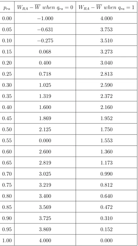
Table 6. The values of the di¤erence between the average …tness of the risk aversion of young population and the average …tness of the entire population for di¤erent proportion levels of risk averse youngs and only risk seeking olds, qra = 0
or only risk averse olds, qra = 1
pra WRA W when qra= 0 WRA W when qra = 1 0:00 1:000 4:000 0:05 0:631 3:753 0:10 0:275 3:510 0:15 0:068 3:273 0:20 0:400 3:040 0:25 0:718 2:813 0:30 1:025 2:590 0:35 1:319 2:372 0:40 1:600 2:160 0:45 1:869 1:952 0:50 2:125 1:750 0:55 0:000 1:553 0:60 2:600 1:360 0:65 2:819 1:173 0:70 3:025 0:990 0:75 3:219 0:812 0:80 3:400 0:640 0:85 3:569 0:472 0:90 3:725 0:310 0:95 3:869 0:152 1:00 4:000 0:000
The e¤ect of changes in the structure of the matching process shows that if there exist only risk averse olds in a population, then risk aversion exactly arises among the youngs. Similarly, if there exist only risk seeking olds in a population, then the evolution of risk aversion among the youngs depends on the level of the proportion of risk averse youngs; the level of playing the mutant strategy would increase, decrease or stay the same.
Now, we can consider the e¤ects of the mutation on the population structure by means of the agents’intertemporal strategy choices. For this purpose, …rst suppose that the age groups choose their actions which lead them to the payo¤ dominant equilibrium as in economics literature argument. Hence, let the population be con-stituted by risk seeking youngs and risk averse olds at time t = 0: Let prs = 0:90
and qra = 0:90: Then, we expect a rise in number of the risk averse youngs and
risk seeking olds at t = 1. Let take these new higher proportions as pra = 0; 90
and qra = 0:10 at t = 1. Then, we observe the reverse at t = 2, i.e., risk aversion
decreases among the youngs. This means that, for this given game, under given initial mutant proportions below, risk dominancy ‡uctuates.
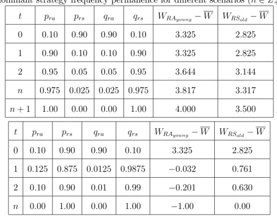
Table 7. Intertemporal analysis of risk dominant strategy frequency and payo¤ dominant strategy frequency permanence for di¤erent scenarios (n 2 Z+)
t pra prs qra qrs WRAyoung W WRSold W 0 0:10 0:90 0:90 0:10 3:325 2:825 1 0:90 0:10 0:10 0:90 3:325 2:825 2 0:95 0:05 0:05 0:95 3:644 3:144 n 0:975 0:025 0:025 0:975 3:817 3:317 n + 1 1:00 0:00 0:00 1:00 4:000 3:500 t pra prs qra qrs WRAyoung W WRSold W 0 0:10 0:90 0:90 0:10 3:325 2:825 1 0:125 0:875 0:0125 0:9875 0:032 0:761 2 0:10 0:90 0:01 0:99 0:201 0:630 n 0:00 1:00 0:00 1:00 1:00 0:00
t pra prs qra qrs WRAyoung W WRSold W
0 0:05 0:95 0:05 0:95 0:301 0:548
1 0:03 0:97 0:01 0:99 0:707 0:232
2 0:01 0:99 0:005 0:995 0:888 0:088
n 0:00 1:00 0:00 1:00 1:00 0:00
Hence, if we analyze a population when it is in its general risk taking behavior pattern such that one group leaves playing risk dominant strategy and the other group continues on choosing its risk dominant action, then we conclude that at the end mutation become extinct for the payo¤ dominant equilibrium biased group.
Thus, this enable us to obtain the threshold levels of population proportions to observe a risk dominancy continuousness in the subject population and vice versa.
CHAPTER 5
CONCLUSION
In this study, we have applied evolutionary game theory techniques to solve a 2x2 coordination game which has one payo¤ dominant and one risk dominant equilibrium in a model including youngs and olds populations to analyze their risk taking behaviors. We have …rst solved a benchmark model by taking the population homogeneous in terms of age. Hence, we made the calculations for the games which are played between only young agents and between only old agents. Then, we derived the necessary conditions depending on the introduced payo¤ levels for risk dominant strategy invasion for both youngs and olds populations.
In the second step, we have introduced heterogeneity into the benchmark model. We stated the possibilities of matching between di¤erent age groups in this setup and reached the equations that promote evolution in terms of risk taking behavior of agents. Then, we derived the open form analytical levels of the payo¤s which guarantee that for a given population, members would focus on choosing the risk dominant action. We also provided numerically the e¤ects of the initial …tness level, initial risk averse and risk seeking proportions on the pattern of the evolution process. We …nd that decrease in initial level of …tness increases the mutation. Moreover, we concluded that in a population the olds of which are only risk averse, mutation increases in time among the youngs. However, in a population the olds of which are only risk seeking, there exists an initial risk aversion threshold for the youngs population to promote risk aversion among them.
Finally, we studied the intertemporal e¤ects of di¤erent risk averse and risk seeking population proportions on mutation. We showed that it is possible to …nd a spesi…c initial mutation proportion which guarantees the further mutation continu-ousness or ‡uctuations on mutation. Moreover, in a population if one group leaves playing risk dominant strategy and the other group continues on choosing its risk dominant action, then we concluded that mutation become extinct for the payo¤ dominant equilibrium biased group.
Further extensions could be considered by applying di¤erent matching processes which allow risk taking attitude switches. In this case, the possibility for matching of players could be taken di¤erent for di¤erent population groups such that some features like distance, neighborhood or social status would play a deterministic role on the possibilities. This is appropriate to describe situations where players interact only with some spesi…c players. Also, exogeneous variables that promote strategy deviations could be included covering framing e¤ect and sunk cost fallacy which would have e¤ect on the di¤erence between the payo¤ levels since people evaluate these payo¤s with respect to their own lose understanding. Another important question is how even small changes in Arrow-Pratt measure of relative risk aversion (RRA) do a¤ect the decision process of agents. By using a three-period OLG Model in which agents are heterogeneous with respect to their ages, as well as their risk attitudes, we would work with not constant inter-temporal elasticity of substitution as usual. RRA would vary across the agents such as (t); (t+1); (t+2) where (:) is the inter-temporal elasticity of substitution (the inverse of relative risk aversion measure). Hence, with respect to this link between time and risk aversion measure, the intertemporal mutation behavior of a population would be studied in detail and would be included in OLG framework endogeneously. Moreover, age distribution could be detailed by adding more age intervals to the analysis. Finally, by increasing the number of agents, the interactions among agents could be analyzed.
BIBLIOGRAPHY
Mohr, P.N.C., Biele, G. and Heekeren, H.R. 2010. "Neural Processing of Risk," The
Journal of Neuroscience 30(19): 6613-6619.
Strough, J.N. and et al. 2008. "Are Older Adults Less Subject to the Sunk-Cost Fallacy Than Younger Adults?," Psychological Science 19(17): 650-652.
Janssen, M.A. and Scheffer, M. 2004. "Overexploitation of Renewable Resources by Ancient Societies and the Role of Sunk-Cost Effects," Ecology and Society 9(1): 6.
Stahl, D.O. and Huyck, J.V. 2002. “Learning Conditional Behavior in Similar Stag Hunt Games.” Working Paper. Wharton University of Pennsylvania, Philadelphia.
Halek, M. and Eisenhauer, J.G. 2001. "Demography of Risk Aversion," The Journal
of Risk and Insurance 68(1): 1-24.
Klaczynski, P.A. 2001. "Framing Effects on Adolescent Task Representations, Analytic and Heuristic Processing, and Decision Making: Implications for the Normative/Descriptive Gap," Journal of Applied Developmental Psychology 22(3): 289-309.
Cunha-e-sa, A.M. and Reis, A.B. 2007. “The Optimal Timing of Adoption of a Green Technology,” Environmental and Resource Economics 36: 35-55.
Schützeichel, J. and Michl, T. 2010. “A Neuroeconomic Perspective on Age and Risk-taking Behavior.” Paper presented at LabSi Conference on “Neuroscience and Decision-Making,” held in University of Siena, Santa Chiara, Italy, September 20,21.
Weibull, J.W. 1998. “What Have We Learned from Evolutionary Game Theory So Far?.” Working Paper 487. The Research Institute of Industrial Economics IUI, Sweden.
Mailath, G.J. 1998. "Do People Play Nash Equilibrium? Lessons from Evolutionary Game Theory," Journal of Economic Literature 36(3): 1347-1374.
Friedman, D. 1998. "On Economic Applications of Evolutionary Game Theory,"
Wang, H. and Hanna, S.D. 1997. "Does Risk Tolerance Decrease With Age?,"
Financial Counseling and Planning 8(2): 1-6.
Jagannathan, R. and Kocherlakota, N.R. 1996. "Why Should Older People Invest Less in Stocks Than Younger People?," Federal Reserve Bank of Minneapolis
Querterly Review 20(3): 11-23.
Kandori, M., Mailath, G. and Rob, R. 1993. "Learning, Mutation, and Long Run Equilibria in Games," Econometrica 61(1): 29-56.
Ellison, G. 1994. "Learning, Local Interaction, and Coordination," Econometrica 61(5): 1047-1071.
Harsanyi, J. and Selten, R. 1988. A General Theory of Equilibrium Selection in
Games. Cambridge, MA: MIT Press.
Morin, R.A. and Suarez, A.F. 1983. "Risk-aversion Revisited," The Journal of