Image processing with the fractional Fourier transform: synthesis, compression and perspective projections

irVîAGE PI%OC€SSİHG WITH THE ERACT80NAİ.

C O M PR E SSIO N AND PERSPECTIVE PR O JE C T IO N S

A T H E S IS S U B M IT T E D T O T H E D E P A R T M E N T OF E L E C T R IC A L A N D E L E C T R O N IC S E N G IN E E R IN G A N D T H E IN S T IT U T E OF E N G IN E E R IN G A N D S C IE N C E S OF B IL K E N T U N IV E R S IT Y l a N ; P A R t l A L · F U L R L f^ M E N T O i.:T H E R EQ U FOR'^THE D E G R E E OF x--: ■ M A S T .iR -'O F 'S C IE N C E ^

L.Ş'ami! Yetik

IMAGE PROCESSING WITH THE FRACTIONAL

FOURIER TRANSFORM: SYNTHESIS,

COMPRESSION AND PERSPECTIVE PROJECTIONS

A THESIS

SUBMITTED TO THE DEPARTMENT OF ELECTRICAL AND ELECTRONICS ENGINEERING

AND THE INSTITUTE OF ENGINEERING AND SCIENCES OF BILKENT UNIVERSITY

IN PARTIAL FULFILLMENT OF THE REQUIREMENTS FOR THE DEGREE OF

MASTER OF SCIENCE

By

i. Şamil Yetik

August 2000

QA 4 o 3 S

' H i -2.000

I certify that I have read this thesis and that in my opinion it is fully adequate, in scope and in quality, as a thesis for the degree of Master of Science.

Prof. Dr. Haldun M. Özaktdş (Supervisor)

I certify that I have read this thesis and that in my opinion it is fully ad<xiuat(i, in scope and in quality, as a thesis for the degree of Master of Science.

Prof. Dr. A. Enis Çetin

I certify that I have read this thesis and that in my opinion it is hdly adequate, in scope and in quality, as a thesis for the degree of Master of Science.

Assist: Prof. Hy. Murat Alanyali

Approved for the Institute of Engineering and Sciences:

Proh Dr. MeSinet Вам

Director of Institute of Engineerii^^and Sciences

A B ST R A C T

SIGNAL PROCESSING APPLICATIONS OF THE

FRACTIONAL FOURIER TRANSFORM

i. Şamil Yetik

M. S. in Electrical and Electronics Engineering

Supervisor: Prof. Dr. Haldun M. Özaktaş

August 2000

In this work, first we give a summary of the fractional Fourier transform including its definition, important properties, generalization to two-dimensions and its discrete counterpart. After that, we repeat the concept of filtering in the fractional Fourier domains and give multi-stage and multi-channel filtering configurations. Due to the nonlinear nature of the problem, the transform orders in fractional Fourier domain filtering configurations have usually not been optimized but chosen uniformly up to date. We discuss the optimization of orders in the multi-channel filtering configuration. In the next part of this thesis, we discuss the application of fractional Fourier transform based filtering configurations to image representation and compression. Next, we introduce the fractional Fourier domain decomposition for continuous signals and systems. In the last part, we analyse perspective projections in the space-frequency plane and show that under certain conditions they can be approximately modeled in terms of the fractional Fourier transform.

Keywords: Fractional Fourier transforms, signal and system synthesis, image representation and compression, perspective projections.

ÖZET

KESİRLİ FOURIER DÖNÜŞÜMÜNÜN

SİNYAL İŞLEME UYGULAMALARI

i. Şamil Yetik

Elektrik ve Elektronik Mühendisliği Bölümü Yüksek Lisans

Tez yöneticisi: Prof. Dr. Haldun M. Özaktaş

Ağustos 2000

Bu çalifjimula, önce kesirli Fourier dönüşümünün bir özeti verildi. Bu özetde, kesirli Fourier dönüşümünün tanımı, önemli özellikleri, iki boyuta genellenmesi ve sayısal kesirli Fourier dönüşümünün tanımı vınildi. Daha sonra, kesirli Fourier dornenlerinde süzgeçleme ve çok kanallı ve çok kademeli süzgeçleme düzenekleri tanımlandı. Bu düzeneklerde doğrusal olmayan bir yapı gözlendiğinden, bu zamana kadar dönüşüm dereceleri düzgün dağılımlı olarak alınmıştı. Bu çalışmada, bu dereceler üzerinden iyileştirmeyi sağlayan bir yöntem sunuldu. Bir sonraki bölümde, kesirli Fourier dönüşümü süzgeçleme düzeneklerinin görüntü sıkıştırılması alanında kullanımı gösterildi. Daha sonra, devamlı işaretler için kesirli Fourier dorrıen çözümlemesi tanımlandı. Son olarak, perspektif izdüşüm uzay-sıklık düzleminde incelenerek, perspektif izdüşüm ih; kesirli Fourier dönüşümü arasındaki ilişki irdelendi. Belli şartlar altında, kcisirli Fourier dönüşümü kullanılarak, perspektif izdüşümünü yaklaşık olarak elde etmenin bir yöntemi verildi.

Anahtar Kdimder: kesirli Fourier dönüşümü, işaret ve sistem sentezi, görüntü sıkıştırılması, perspektif izdüşüm.

A C K N O W L E D G M E N T S

I would lik(! to express riiy deepest gratitude to Prof. Dr. Haldun M. Ozakta^ for his excellent supervision, guidance, suggestions and endless patience.

I would also like to thank the members of my committee. Prof. Dr. A. Enis Çetin and Assist. Prof. Dr. Murat Alanyah for their comments on the thesis.

Finally and mostly, I want to express my sincere and deepest thanks to rny family for their endless support throughout my education.

C on ten ts

1 Introduction 1

2 The Fractional Fourier Transform 5

2.1 Introduction and H isto ry ... 5 2.2 Definition and P roperties... 7

3 O ptim ization of Orders in M ulti-C hannel Fractional Fourier

Dom ain Filtering Configurations 12

3.1 Filtering Configurations Based on the Fractional Fourier Transforin 12 3.2 Optimization of Orders in the Multi-Channel Filtering Configuration 15

4 Image R epresentation and Compression w ith the Fractional

Fourier Transform 23

5 Continuous Fractional Fourier Domain D ecom position 27

6 Perspective P rojections and Fractional Fourier Transforms 29

6.1 Introduction... 29 6.2 P(',rsp(ictive P rojections... 30 6.3 Pcirspective Projections and Fractional Fourier Transforms 33 6.4 Error A nalysis... 41

7 Conclusions and Future Work 47

List o f Figures

2.1 The iractiorial Fourier transforms of a rect with a continmim of

orders 9

3.1 Fractional Fourier transform based filtering configurations 14 3.2 Gaussian Schell-model mutual intensity synthesis 19 3.3 Rectangular mutual intensity sy n th e s is... 21 4.1 Iinag(! compression e x a m p le ... 2G 6.1 Perspective m odel... 31

6.2 VVigmu· distribution of an exponential and a c h i r p ... 33

6.3 Illustration of the decomposition of the approximation into (derrumtary operations in the space-frequency plane 35 6.4 Persp(!ctive proj(!ction approximation: example 1 37 6.5 Ihuspectivii projoiction approximation: example 2 38

6.6 2D Persi)cctive m odel... 39 6.7 2D Perspective projection approximation: example 42

6.8 Gomparison of VVigner distributions underlying error analysis . . . 44 6.9 Valid regions of the perspective projection approxim ation... 45

C hapter 1

In trod u ction

Digital signal processing has found a central place in signal processing after the popular use of digital computers in various applications, where oikí needs

to process signals for many purposes like transmitting, storing, compressing, enhancement and many others. Some of the .systems of the processes mentioned above are non-linear, some of them are linear. However, linear systiuns are (iasy to handle and in some applications they constitute a group of systems that is adequate lor many purposes. Linear systems can also be used to model non­ linear .systems. Boicause of these reasons, linear systems have been extensively emphasiz(!(l in digital signal processing.

A general linear .systtnn can be characterized as.

g(u) = I H{u,u' )f{u') du\ ( f . l )

where H{v., u') is called the kernel of the system and g{u) and /(n ) a.re the output and input of the system, respectively. Discrete version of 1.1 can be expresscid as,

N - l

(

.

)

s{n] = f : H i n , k ] m , k=Q

where fj[n] and f[n] are either samples of f{u) and g{u) or discrete functions that somehow occur in digital systems, and H[n, k] are either samples oi H{u, u')

or the kernel of a digital .system. The last equation is simply a matrix vector multiplication which can also be written as,

g = H f, (1.3)

where g and f ai(i vectors representing ()[n] and /[n] and H is a, rmitrix representing /i[n, A:]. A detailed discussion of the signals and systems may be found in [1,2].

In many a.pplications, we face with linear systems that are shift-invariant. In the case of shift-invariant systems, when the input is shifted l)y a cfutain amount, the output is also shifted by the same amount. This property is equivalent to having a kernel of the special form H{u,u') = h{u - u'). Fourier transform is a very powerful tool in analyzing shift-invariant systems, because shift-invariant systems correspond to a multiplication in the Fourier domain. Turning our attention to the digital case, matrices representing the shift-invariant digital s3^sterns are circulant matrices and the Fourier transform matrix (DFT) diagonalizes the kernel matrix. There exists a fast algorithm (FFT) that allows us to compute Fourier transform in 0{ N\ogN) time (Here N is the length of the discrete signal vectors or the time/space-bandwidth product of continuous signals). This efficient implementation is the main reason that Fourier transform plays a central roh; in the analysis of shift-invariant systems.

We can think of the general linear systems and shift-invariant linear systems as the two extremes. In one end, implementation cost is 0{ N\ogN) (shift- invariant syst(uns), and in the other end, implementation cost is 0 ( N ‘^) (general linear systems). In some applications, shift-invariant systems may be inadeciuate but efficient, and general linear systems may be adequate but inefficient. This situation suggests to search for a way to be able to trade-off between cost and performance. One way which makes this trade-off possible is the use of fractional Fourier transform. The fractional Fourier transform is a generalization of the ordinary Fourier transform; definition and some of its properties will be given in

the next chapter.

The original contribution of this thesis to the research area is summarized in this part. The optimization of orders in fractional Fourier transform has not been addressed before, in this thesis we have given a method to optimize orders in the multi-chanii(!l filtering configuration. Although fractional Fouricu' transform bas(xl hltering configurations are used in systern/signal synthesis, signal resl.oration and feature extraction, the idea of using fractional F'ouriiu· transform Irased filtering configurations in image representation and compr(',ssion is introduced in this thesis, for the first time. Continuous counterpart of fractional Fourier domain decomposition is defined. Finally, relation between persjKîctive projections and fractional Fourier transforms are also studied in detail, and it is shown that perspective projections can be approximated by fractional Fourier transforrns under certain conditions.

In Chapter 2, we give the definition of the fractional Fourier transform and some of its important properties. Also, we are going to giræ a brief history of the fractional Fourier transform and mention some of the applications where the fractional Fourier transform is used. In Chapter 3, we give the conccipt of filtering in fractional Fourier domains and represent the multi-stage and multi-channel filtering configurations. Also, we discuss the optimization of fractional Fourier transform orders for multi-channel filtering configurations by first finding the optimal filter coefficients for a larger number of uniformly chosen ordcus, and then maintaining tlu! most important ones. Chapter 4 is reserved for the discussion of the application of fractional Fourier transform based filtering configurations to image repiiisentation and compression. In Chapter 5, w(! defiiui continuous version of fractional Fourier domain decomposition, of which the discrete v(usion and its apirlications were studied before.

In Cha,[)ter 6, we arial.yse perspective projections in the space-fr(Kiuenc,y plane and show that under certain conditions they can be approximately modeled in terms of the fractional Fourier transform. Conclusions and future work are discussed in Chapter 7.

C h ap ter 2

T h e Fractional Fourier Transform

2.1

Introduction and H istory

The fractional Fourier transform is a one-parameter generalization of the ordinary Fourier transform. We obtain the fractional Fourier transform l>y using this parameter as the functional power of the ordinary Fourier transform.

The fractional Fourier transform is introduced to the mathematics community by the early papers [3 5]. However, it did not draw much attention until it has been used by o|)tics and signal processing communities. Number of publications has exploded after 1980’s when it has found its place in optics and signal processing.

The fractional Fourier transform suggests a potential improvcunent in tlu^ applications where! ordinary Fourier transform is used, since il. provides an <!xtra parameter. We can improve the solution to any problem that had jiievionsly utilized Fouri(!r transform, by carrying the extra parameter throughout tlu! solution and then optimizing over this parameter. We can group the se'veral applications of the fractional Fourier transform as: i) applications in mathematics and physics, ii) optical information processing applications and iii) digital signal proc(!Ssing applications.

In this thesis, we are more interested in signal processing applications of the fractional Fourier transform, however we briefly give some selected publications in other areas as well. Mathematics and physics applications of the fra,ctional Fourier transform [6-8] include quantum mechanics, uncertainty i)rinciples and solution to differential equations. Optics applications of the fractional Fourier transform [9 16] include optical propagation and diffraction, anal5^sis and design of Fourier optical systems, beam shaping and other applications.

Fractional Fourier domains are first introduced in [17], and many applications of the fractional Fourier transform has been based on this concept. Oi)timum Wiener filtering in fractional Fourier domains are studied in [18]. In this paper, analytic solutions are presented that yield the optimum fractional Fourier domain and optimum filter coefficients corresponding to this domain. As an application of the optimal filtering in fractional Fourier domains, optimal image restoration is studied in [19]. In these papers, a single fractional Fourier domain has been used. The concept of generalizing the fractional Fourier domain filtering to two or more number of domains has been studied in two directions mostly. First one is multi-stage filtering, which is defined as filtering in consecutive fractional Fourier domains, and has been studied in [20]. Multi-stage filtering has found applications in signal restoration [20], system synthesis [21], mutual intensity synthesis [22]. Se(;ond one is multi-channel filtering, which is defined as filtering in parallel fractional Fourier domains in [23]. Multi-channel filtering has been used in system decomposition [24,25]. In [24], fractional Fourier domain d(;composition is defined and its applications like efficient implementations of linear systems are given. Other applications of multi-channel filtering including signal recovery and restoration, signal synthesis and system synthesis has been studied in [23]. Continuous version of fractional Fourier domain decomposition is dehned in [25]. The fractional correlation is first defined in [26] and developed in [27]. The concept of fractional correlation is used in pattern recognition in [28,29]. Also, feature extraction using the fractional Fourier transform can be found in [30].

Some of the other references related to the fractional Fourier transform and its applications can be listed as [31-41].

Here, we do not give the complete list of references, for a morci complete list one can refer to [2].

2.2

D efinition and P roperties

The ath order fractional Fourier transform of the function /(« ) will be denoted by faiu)· Here, we are going to give the linear system kernel definition of the fractional Fourier transform. Other equivalent definitions can be found in [2]. The fractional Fourier transform of a signal is defined as:

M u ) = I K.{u,u' )f(u' )du' , Kai'll", u') = A,j, exp |^i7r(cot (j) — 2 esc (f> uu' + cot 4>

(2.1)

where

, air

(2.2) A,j, = \jl — i cot (j). (2,3) The square root is defined such that the argument of the result lies in the interval (—7t/2, 7r /2j. When a is an even integer the above kernel is undefined. However, it is possible to show that as o, approaches an even integer, the kernel approaches a delta function. That is, Kij{u,u') = 6{u - u') and K^j±2{u.,u') - + ■(/,'), where j is an arbitrary integer.

Now, we are going to give some special cases of the fractional Fourier transform. The fractional Fourier transform is equal to the identity operation when a -- 0, to the ordinary Fourier transform when a = 1, to the parity op(!ration when a — 2 and to the inverse Fourier transform when a — 3. Close, examination of the kernel given in 2.1 reveals that the fractional Fourier transform is periodic in a with period 4. The fractional Fourier transform interpolates between tin; 0th

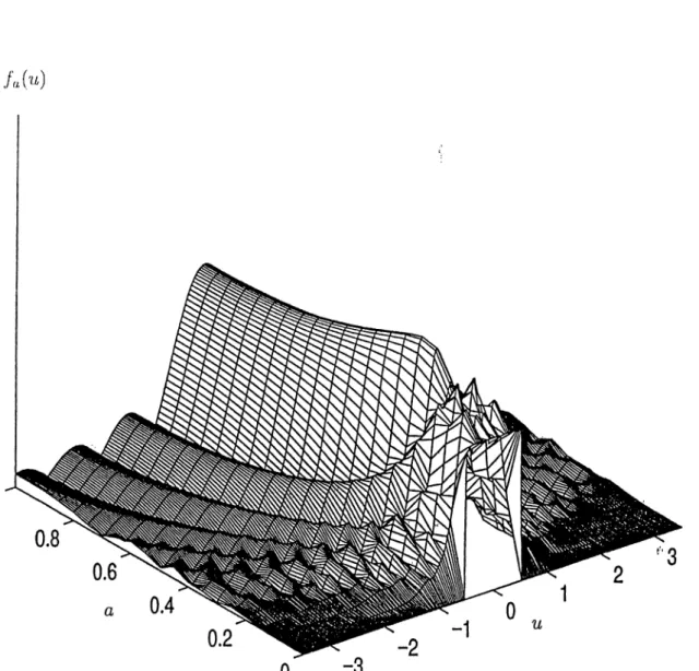
order fractional Fourier transform (original function) and the 1st order fractional Fourier transform (ordinary Fourier transform of the signal). This is illustrated for a rect function in Figure 2.1.

Having given the definition, now we are going to have a look at Hie important Iiroperties of the fractional Fourier transform, briefly. First, the fractional Fourier transform is a one iiarameter generalization of the ordinary Fourier transform and it is a member of the linear canonical transforms. Another important profierty of the fractional Fourier transform is index additivity. That is, aith order fractional Fourier transform of the «,2th order fractional Fourier transform is ecpial to the

(04 + a2)th order fractional Fourier transform. Relation between the fractional Fourier transform and the Wigner distribution is of central importance in many applications. Before giving this relation, we are going to give the definition and some important properties of the Wigner distribution here for convenience.

The Wigner distribution Wf{u,n) of a function f{u) is defined as

Wfiu, fi) =

I

|/(.u

)|2

=

J

W/(u,/r)

I Wf{u,^i)d.u,

E n [ / ( 'u ) ] = I Wf(u, fi) dudfj,,

(2.5)

(2.6)

(2.7)

En[/(u)] is the total energy of the signal f{u). These properties reveal that Wigner distribution gives the distribution of the signal energy over space and frequenc,y. The Wigner distribution of F'(/i), is a ninety degree rotated version of the Wigrier distribution of ,f{u). More on the Wigner distribution and other such distributions and representations may be found in [42].

fa(u)

Figure 2.1; Axis ranging from 0 to 1 indicates the fractional Fourier transform order. Each slices of this three-dimensional figure corresponds to the fractional Fourier transform of the rect function with a certain order. Wh(iii a == 1, we observe the Fourier transform of the rect: a sine (After [48]).

If Wf(u,iJ,) d(!iiotes the Wigner distribution of f{u), then the Wigner distribution of the ath order fractional Fourier transform of f{u), denot(id l)y Wfju,fi), is given by:

W/■„ (u, ft) = Wf (u cos Ф — (Л sin Ф, и sin Ф + fi cos Ф), (2.8)

that is, the Wigner distribution of /„('u) is the clockwise rotated version of thci Wigner distril)ution of fin) by an angle 4>. A result of this property is as follows:

/ W ! j n , ^ ) d ^ = \ U n ) ? . (2.9) That is, the integral projection of the Wigner distribution of a function onto the Щ axis is equal to the magnitude square of the ath order fractional Fourier transform of the function.

Finally, there exists a fast implementation of the fractional Fourier transform [43] with implementation cost 0{N\og{N) ) . Actually, this fast implementation makes it i)ossible to use the fractional Fourier transform in applications where the ordinary Fourier transform is used, with no additional cost, resulting in possible improvements. However we should note that, this fast implementation cannot be interpreted as the discrete fractional Fourier transform, because it does not satisfy important properties like index additivity and Wigner rotation property, exactly.

Discrete fractional Fourier transform is defined in [44]. The discrete fractional Fourier transform satisfies the properties of the continuous fractional Fourier transform. But, an efficient implementation of the discrete fractional Fourier transform has not been found up to this date.

Until now, we have considered only the one-dimensional definition of the fractional Fourier transformation. Here, we will generalize the definition of the fractional Fourier transform to two-dimensions. There are two ways of generalizing the definition to two-dimensional systems.

First one is the separable two-dimensional fractional Fourier transform defined as:

/.(q) =

¡...M =

^“/(q) =

= j j Ka,,,u.{u,v,u\v')H:u,\ v')du'dv\

(2.10)

for two dimensions and similarly for higher dimensions. Here q = viu + vv a.nd a = a„u-|-a^v where ii and v are unit vectors in the u and v directions. Kai'ii·, 'ti')

is the one-dimensional kernel defined in equation 2.1.

Second one is the non-separable two-dimensional fractional Fourier transform defined as /citetwod: / 00 -00 where (q, q") = Kq exp['f7r(q'^Aq + 2q^Bq" + q"'^Cq")] (2.11) (2.12) with r T r 1 A q — K y/ K y !, r U V , q " = u " v " T A = cot (¡)yi 0 0 cot (/)yi B COS O2 CSC sin 0i CSC (p^, f COs(^l-6/2) COs(0i-(?2) sin O2 CSC (p^,t _ cos 0l CSC (f) t

COs(^l-02) COs(0i/?2)

-c =

con-O2 ....f J, I nm^O’2 rni-fh ; sin cos (92 r n f rh : 4- sin 0'2 f.f.f A .

conHO,-(h) W + COS’^(0 l - 02) cos‘^ (0 i-0 2) ^ COS-^(0l-02)

sill0 J cos 02 A 1 sin 02 COS 01 ,,^4. ^ . COS^ 0] ^.^4. ^ . j ____ Siir' 0]___ ,

L “ COS*^(0, -02) COS-^r01-02) COS‘^(0i-02) ^ COs’^ (01-02)

Here we give the definitions of the fractional Fourier transform for tlui salui of completeness. These two-dimensional fractional Fourier transforms will not be employed in this thesis.

C h ap ter 3

O p tim ization o f Orders in

M u lti-C h an n el Fractional Fourier

D om ain F ilterin g C onfigurations

3.1

F iltering C onfigurations B ased on th e Frac­

tional Fourier Transform

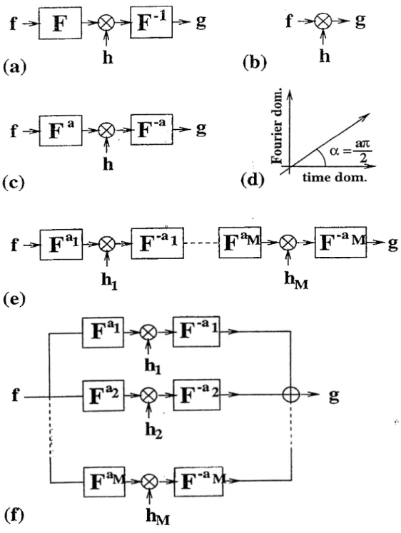
Space- and freciuency-dornain filtering are special cases of fractional Fonrier domain filtering (3.1(a,h,c)) [18,46]. Fractional Fonrier domain filtcuing consists of (i) taking tlici fractional Fourier transform of the input signal, (ii) multiplication with a filter function, and (iii) taking the inverse fractional Fourier transform of the result. Tlui fractional version of the optimal Wiener filtering ])rohlem has been studied in detail in [18]. Fractional Fourier domain filtering has been further gciueralized to midti-stage and multi-channel filtering (3.1 ((>,f)). In multi­ stage filtering [21,47] the input is first transformed into the oi th domain, where it is multi[)li(!(l 1)3^ a filter hi. The result is then transformed back into the original domain. This process is repeated M times. Denoting the diagonal matrix

corresponding f.o inultiplication by the kth filter by A^, we can writii the following expression for the overall effect of the multi-stage filtering configuration:

(3.1) where T ,i,h i« a matrix representing the overall multi-stage filtering configuration and F “*' denot(',s the discrete fractional Fourier transform matrix [44]. Multi­ channel filtering configurations [24,47] consist of M single-stage blocks in ])arallel. For each chaniKd k, the input is transformed to the a^kth domain, nndtiplied by a filter hk and then transformed back. Now, we can write the following expression for the oviuall effect of the multi-channel filtering configuration:

T _{-L m} r —

-M

^ F - “'=AfcF“*^

LA;=1

(3.2)

where T„„·, is a matrix representing the overall multi-channel filtering config­ uration. It is i)ossible to further generalize these filtering configurations by using parallel and series arrangements together; such systems have been called generalized filtering circuits [47,48]. The problem of finding the optimal filter coefficients, given the transform orders, has been solved in [18,21,47]. Given a matrix H which represents a system one wishes to synthesizci, one seeks the filter coefficients such that the resulting matrices T ^s or T„,c is as c;lose as possible to H according to some specified criteria, such as mean s(iuare error. Until now, the transform orders have usually been chosen uniformly (a, = 1/M, 0-2 = 2/M, ...o,M = 1); the problem of optimizing the orders has not yet been addressed. In this chapter, we show how one can optimize over the orders

A A A for multi-channel filtering by first finding the optimal filter coefficients for a larger number of uniformly chosen orders, and then maintaining the most important ones.

In [21,24,47] fractional Fourier transform based filtering configurations have been used for approximating linear space-variant systems, represented by some

(a)

F

h

-1

f

S

(b)

h

Z l r f ■

h

F

(C)

(e)

(f)

F '

h.

h

Figure 3.1: a) Fourier domain filtering, b) Space domain filtering, c) ath order fractional Fourier domain filtering, d) ath order fractional Fourier domain, e) Multi-stage filtering, f) Multi-channel filtering. (After [22])

matrix H. It was shown that for many such systems encountered in various applications, it is possible to approximate the system H with a multi-stage or multi-channel conhguration T„ik or T,n(; with acceptable mean square (uror, by using a small or rnoderatii number (M) of stages or channels. Since the cost of implementing the fractional Fourier transform (optically or digitally) is similar to the cost of implementing the ordinary Fourier transform, this hiads to a. fast implementation of the space-variant system in question. For instance, for digital systems, the cost becomes O(AdNlogN), which should be comparcxl to the cost 0{N'^) for direct implementation of linear systems.

In the multi-channel case it is possible to analytically find the optimal filter coefficients, provided the transform orders are given. In practi(;e, however, an iterative method is preferred. In the multi-stage case it is not possible to find analytic solutions, so an iterative method must be used to begin with.

3.2

O ptim ization o f Orders in th e M ulti-

C hannel Filtering C onfiguration

In this section, we concentrate on the multi-channel filtering case, and consider the improveriKmt of optimizing over the M orders in addition to the filter coefficients. We first hnd the optimal filter coefficients for a larger nnmber P of uniforiidy chosen orders and then maintain the most important ones. More specifically, w(' start with P uniformly chosen orders, where P is several tiimis the number of orders M we are eventually going to use. Then the M ord(;rs resulting in filters with the highest energies are chosen, and the other P — M l)ranches of the multi-channel configuration are eliminated. Finally, with the M orders thus chosen, we reoptimize the filter coefficients. Here, we should note that the method proposed does not give the global optimum for the orders but gives the orders that provides imi)rovements compared to uniformly choosing tlui orders.

As an (ixainple, we will consider the problem of synthesizing light with a desired inntual intiuisity. Here we wish to synthesize a system H such that, when light of giv(ni rnutnal intensity is present at the input, light wdiose mutual intensity is as close as possible to the given specification is obtained at tlu! output. Choosing to work with one-dirnensional signals for simplicity, w(' let f{x) and (j{x) denote the input and output optical fields, and i?,/(.г■|,.T2) and

denote tlui input a.nd out[)ut mutual intensities. If f{ x) and (j(x) are the input and output of a system characterized l)y a kernel H{x,x' ) such that <]{x) = J H{ x, x' ) f{ x' ) dx', then the input and output mutual intensities ata; related by

B,f,{xi,X2) =

I J

R^ = H R /R t, (3.4)

where is tlie Herrnitian conjugate of H. Equation 3.4 is (piadratic in H. VV(; are going to employ an eciuivalent representation which is linear. Since inutTial intensity matrices R are Hermitian and positive serni-definite, it is possible to diagonalize them as

R = U D U t, (3.5)

where D is a diagonal matrix whose elements are the real eigenvalues, and U is a matrix whose columns constitute the set of orthonormal eigenvectors of R so that U^U = I, where I is the identity matrix. Letting denote the diagonal matrix whose (dements are the positive square roots of the elements of D, w(; substitute for D in the above equation:

R = U D ^ /^ u tu D i/^ u ^ (3.6) 16

Now, using this expansion for both and R/·, we can write equation 3.4 as

R/· = RyRy: = RyRy -- Ry,

(3.7)

where

R^ = R j = UD^/'^^Ut R^ = R} = UD^/^U^

Substituting 3.8 into 3.4 we obtain the following:

R ^R j = H R y R |H ^

One way of satisfying the above equation is to ensure that

R^ = HRy, (3.8) (3.9) (3.10) or H = R gR 7^ (3.11)

In our nuinerical examples, we are going to consider the input light source to be incoherent. Assuming this source extends uniformly from -vo to ro, its mutual intensity can l)e written as

Ry(.r,,.'i';2) = i(.T] - .x-2)rect ) . (3.12)

When discretized, the corresponding matrix Ry (and its square root Ry) is e(iual to the identity I, i)rovided tq is larger than the interval over which we sample.

Therefore!, the matrix H we wish to approximate is simply equal to R^,.

As a hrst example, we wish to synthesize a Gaussian Schell-model beam with mutual intensity:

R,,{x i,X2) = exp ( --- ---j exp

\^-(xi - .X'2)^'^ f x'i +

2r.? (3.13)

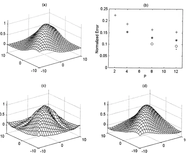
(In our exami)l(iH ri = 5 and 72 = 10, in suitable units.) When we syntlnisize the filter H corresponding to this mutual intensity using the multi-chaniKd configuration with M = 3 filters (ci = 1 /3 ,0,2 = 2/3, a,·) = 1), tlu; norinalized error turns out to be 15.42 %. Using the proposed method of optimizing the orders with P = 12, we find that the optimal orders are 04 - 2/12, (I2 —5/12, a.i =

10/12, and th(i normalized error using these orders becomes 12.64 %. When we synthesize the same H with M = 2 filters (ai = 1/2, 0,2 = 1), the normalized error is 22.36 %. Optimizing the orders with P — 8, we find that the oirtimal orders ar(i a,\ = 2/8, (I2 = 6/8, and the normalized error using tluise orchus is 16.36 %. Further simulations have been undertaken for other values of M and P and th(! result errors are plotted in Figure 3.2(b). Part a of this hgure shows the desired mutual intensity, part c shows the synhthesized mutual intensity for M = 2 without optimization of orders, and part d shows the synthesized mutual intensity for M = 2 with optimization of orders with P = 8.

As a second example, we consider the synthesis, as closely as i)ossible, of a mutual intensity r)rofile specified as

= « c t reel ( | C ) ( | | (3.14)

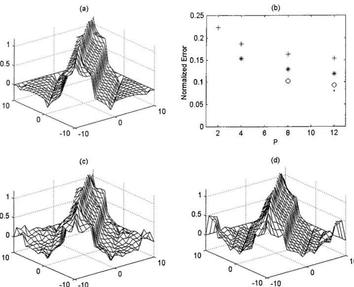
where 72 > r\. This amounts to specifying the amplitude of light at two points to be fully correlated when the distance between those points is less than 27-1, and totally uncorrelated otherwise. Since the rectangle function does not represent a physically realizable mutual intensity function (it is not positive siuni-definite), its negative eigenvalues will be replaced by zero in obtaining its square; root representation. This amounts to replacing the rectangle function with tin', closest positive si'rni-definite function. When we synthesize the filter H corresi)onding to this mutual intensity using the multi-channel configuration with M=3 filters (ai = 1/3, (I2 = 2/3, a,3 = 1), the normalized error is 15.35 %. Using the proposed method of optimizing the orders with P - 12, we find that the optimal orders ar(!

0,1 = 2/1 2,0.2 = 6/12,0,3 = 10/12, and the normalized error using these orders is 18

(a) 10 (c) (d) 1 . 1 -0.5- 0 .5 -0 . 0 -10 10 -10 -10 -10 -10

Figure 3.2: a) Desired Gaussian Schell-model mutual intensity profile, b) Normalized error vs P for different values o f M (M = 2: ’-I-’, M = 4; M = 8: ’o’, M = 12: ’.’). c) Synthesized profile using uniform orders (M = 2). d) Synthesized profile using optimized orders (M = 2, P = 8).

12.3 %. When we synthesize the same H with M=2 filters (ai = ll2,a·) = 1), the normalized error is 22.64 %. Optimizing the orders with P = 8, we hnd that the optimal orders are a.\ = 2/8, 0,2 = 6/8, and the normalized error nsing these orders is 15.45 %. Once again, further simulations have been underta.ken for otlnn· values of M and P and are plotted in Figure 3.3(b). Part a of this figure shows the desired mutual intensity, part c shows the synhthesized mutual intensity for M = 2 without optimization of orders, and part d shows the synth(\sized mutual intensity for M = 2 with optimization of orders with P = 8.

A number of conclusions can be drawn by examining the numerical results. First, optimization of the orders is capable of offering tangible improvements with respect to choosing the orders uniformly. We also observe that beyond a certain value of P , further increases in this parameter do not offer further reductions in the error (the l)enefits of optimizing over the orders is saturated). This is because further increasing P merely allows further refinements and fine-tuning in choosing the optimal orders, which has diminishing return once one moves roughly closer to the optimal orders. Also, we can see that improvements coming from optimization of the orders are greater when M is smaller but less when M is larger. This is because when M is large to begin with, it is already [)ossible to concentrate the filtering action in those domains which are optimal. This of course means that the other domains add cost to the system implementation with litth'. benefit, and the method we propose is useful precisely because it allows these low beruiht domains to be pruned.

In conclusion, we have presented a simple and effective way of optimizing the orders in fractional Fourier domain based multi-channel filtering configurations. Until now, the orders had mostly been chosen uniformly since there was no simple way of solving the nonlinear problem of optimizing over the orders. The nuithod we proposed is niorti likely to be useful when confronted with low-cost, rather than high-accuracy applications, because larger improvements are obtained when tlui use of a snialhu· number of filters is desired. Future work might include extending

(a) (b) 10 0.25 ---- 1----+ ---- 1--- 1--- --- --- 1----0.2 . -L_ -f fc ^ 0.15 . * + + . T)₀₎ .N * * g 0.1 o o o ♦ z 0.05 n ___1___ ___1______ 1 ,

,

Figure 3.3: a) Desired rectangular mutual intensity profile, b) Normalized error vs P for different values of M { M = 2: M = 4: M = 8: ’o’, M = 12: ’.’). c) Synthesized profile using uniform orders (M = 2). d) Synthesized profile using optimized orders { M — 2, P = S).

the method to the multi-stage case, which poses a number of chalhuiges, and to more general iiltering circuits.

C h ap ter 4

Im age R ep resen ta tio n and

C om pression w ith th e Fractional

Fourier Transform

There has been a (.remeiidous amount of work on data compression in general and image comi)ression [49] in particular, leading to efficient compression algorithms. In this cha,pt(ir, we discuss a novel way of representing images based on fractional Fourier domain filtering configurations [47, 48], leading to an image coding method.

In Cha.ptcr 3, we have; introduced the fractional Fourier transform bastvl filtering configurations. Here, we repeat the matrices representing the overall effect of the multi-stage and multi-channel filtering configurations:

(4.1)

T _me

M

^ F - “*'AfeF“*^ (4.2)

LA;=1

In this chapter, we interpret the matrices T,nc and T^s not as represiuiting 23

a linear s.y.stem, but as representing a two-dimensional signal or image. Thus the filtering c.oeffieients in the multi-stage or multi-channel approximation of this matrix, can be used to approximately re[)resent and reconstruct this matrix and the associated image. In other words, the optimal filtering coefficients minimizing the; mean square error between the original matrix and its multi-stage and multi-channel approximation, are taken as the compressed viusion of the image. R(u;onstruction of compressed images is possible in 0 (M N log N ) time. The cited work on synthesis of space-variant systems for fast impleriuuitation shows that satisfactory approximations are possible with rnoderati; nunilxus of filters and hence large reductions in implementation cost. Therefore, it seems worth investigating whether similar approximations with similar reductions in cost (measured by the compression ratio) is possible when these configurations are used for image compression. Since the original image has N'^ luxels and tlu! compressed data has N M pixels, the compression ratio is N /M .

In the multi-channel filtering case, we have also considered the improvement of optimizing over the orders as described in Chapter 3.

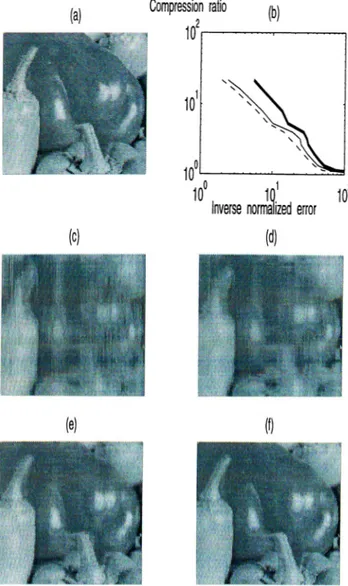
The compression method proposed is tested on the 128 x 128 image shown in Figure 4.1(a). Figure 4.1(b) shows the trade-off between the reconstruction error and compr(',ssion ratio. The mean square error has been normalized by the energy of the original image. The horizontal axis of the plot is the inverse of this normalized error. We see that the multi-channel and multi-stage configurations give comparable results, though the multi-stage configuration is slightly l)(!tter. Optimizing over the orders for the multi-channel case rcisults in tangible improvements.

Figure 4.1(c,d) show illustrative results obtained with the riudti-stage configuration. Although the order-optimized multi-channel case yields smaller errors, we present results for the multi-stage configuration so as to illustrate the performance of the method in its rawest, most basic form. Whereas we ol)serve that nearly an order of magnitude compression is possible with moderate errors.

larger coiiipr(;ssioii ratios are accompanied by larger errors.

Urifortuiiat(ily, we observe that the use of fractional Fourier domain filtering configurations for image compression, does not yield results as good as thos(i obtained when they are used for synthesis and fast implementation of shift-variant linear systems. In its present form, the proposed idea does not yield better rtisults than presently available c:ompression algorithms. However, we em])hasiz(i that the results presented refhict the performance of the basic method in its ra.west and barest form; wc; merely represent the image with the filter coefhcients which make th(i forms giv(ui in (3.1) and (3.2) as close as possible to the image matrix. Further refineiiKint and development of the method and its combination and joint use with other techniciues may lead to full-fledged compression algorithms with bettcu' p(irforniance. Also, it is possible to use the discrete fractional cosine transform which is a real transform, since images we are dealing with arti real and a real transform would therefore reduce the cost. (One way of geiKualizing the method, which can lead to i)otentially higher compression ratios with similar errors is to em[)loy filtering circuits based on linear canonical transforms, rather than fractional Fourier transforms [50].)

Moreover, r(!gardless of the performance that can ultimately be obtained with irnprovenumts of the present idea, the fact that the information inherent in an image and be decomposed or factored into fractional Fourier domains in the manner dtiscribed is of considerable conceptual significance. In a, sens(!, tluise domains “span” a certain space which is a subset of the image space, although the precisi! nature of this is difficult to ascertain in the nonlinear niulti-sta,ge case. The information contained in the image is distributed to the different domains in an uiuKiual way, making some domains more dispensable than othous in repres(uiting the image. Exploring and exploiting these issues se(mi potiuitially rewarding.

Figure 4.1: (a) Original image, (b) Compression ratio vs inverse normalized error: multi-channel (dashed line), multi-stage (solid line), multi-channel with optimized orders (bold line). Reconstructed images with compression ratio 32 (c), 21.3 (d), 8 (e), 5.3 (f). Part c and d represent too much error to be considered compressed versions of the original image. However, they have been shown to illustrate the dependence of the error on the number of coefficients used.

C h ap ter 5

C on tinuous Fractional Fourier

D om ain D eco m p o sitio n

The continuous spectral decomposition (or expansion) and its discrete counter­ part, the singular value decomposition (SVD), plays a fundamental role in signal and system analysis, representation and processing. The spectral decomposition of a function h{u, u') is

CXJ

h{u,u') =

J

In this chapter, we define the continuous fractional Fourier domain decom­ position (FFDD). While the FFDD may not match the spectral decornpo.sitiori’s central importance, we believe it is of fundamental importance in its own right as an alternative which may offer complementary insight and understanding. We believe the FFDD has the potential to become a useful tool in signal and system analysis, representation, and processing (especially in time-frequency space), in some cases in a similar spirit to the SVD.

Let h{u,u') be a two-dimensional function, representing either an image or 27

the kernel of a. one-dirnensional linear system. Its fractional Fourier domain decomposition is defined as

i‘2 /*oo -2 ./ —oo

/■2 roo

h(u,u') = / / K-a{u,u")c{a,u")Ka{u", u') du" da, (5.2)

./ —2 ./—oo

where c(a, u") is a family of one-dimensional weighting functions with parameter a. The integration interval is limited to [-2 2], since the fractional Fourier transform is periodic in a with period 4. We can obtain c(a,u") by solving the integral eciuation 5.2. Sampling this equation we obtain a matrix eciuation which can be solved by using the tools of the linear algebra. Comparing the fractional Fourier decomposition with the spectral decomposition given in (5.1), we can see that the integrands in both expressions consist of three terms. The definition of the FFDD can be rewritten in the form

2 oo

h{u,u') = I ! c{a,u")Pa{u,u',u") dv," da (5.3)

-2 —oo

where we hav(i defined

Pa{u,u',u") = Ka{u",u')K_a{u,'u!') (5.4) Equation (5.3) can be interpreted as an expansion of h(u, u') in terms of the basis functions Pa{u', u", u'") with c{a,u") corresponding to the expansion coefficients.

The basis functions in (5.4) can easily be shown to be linearly indcipendent as a direct consequence of the fact that {Ka{u",u), Ka>{u,u"))u is nonzero for all a, a'. Here {■,■),,. denotes a one-dimensional inner product with respect to tlui variable w.

A natural extension of the FFDD would be the linear canonical domain decomposition (LCDD) based on linear canonical transforms [50].

P ersp ectiv e P ro jectio n s and

Fractional Fourier Transform s

C h ap ter 6

6.1

Introduction

Perspective j)iojectioiis are used in many applications in image and video processing, especially whcm confronted with natural or artificial scenes with depth (for instance, in robot vision applications). Perspective projections can be considered as a geometric or pointwise transformation, in the sense that each point of the ()l)ject is mapped to another point in the perspective projiiction [51-53]. In this chapter we will examine the perspective projection in the spac(!- frequency i)laii(i and show that its effect on the object can be modeled in terms of the fractional Fourier transform [56].

The VVigner distribution of an exponential function exp[i27ri^a·] is a line (hdta lying parallel to the space axis:

W j i x , a , )= S i a , -0 , (6.1) and the VVigner distribution of a chirp function exp[i7r(y.'i;^ + 2i;.7; + ()] is an oblique line delta:

Wf{x, cr,,) = 6{ a^~ XX - 0 ·

To uiuloirstand why the fractional Fourier transform is expected to play a role in perspective projections, let us consider the perspective projection of an image exhibiting periodic features, such as a railroad track. More “distant” parts of the image will appear in the projection smaller than “closer” parts. Thus a periodic or harmonic feature of certain frequency will be mapped such that it (exhibits a monotonie increasing frequency. Under certain conditions, this incr(ias(i can be assuirnul liiKîar so that the harmonic function is mapped to a chirp function. Since fractional Fourier transforms are known to map harmonic functions to chirp functions, we expect that perspective projections can be modeled in terms of fr actional Four ier trarrsforrns. The purpose of this chapter is to forrrrulatri this relationship.

In the next section, we are going to present the perspective model we use and examine the effect of the perspective projection on the Wigner distribirtiorr. In the following section, we will discuss the relation between the fractional Fourier transforrrr and perspective projections based on their effects on the Wigner distribution. We will discuss how perspective projections can lx; rrrodeled as shifted and fractional Fourier transformation. The last section is devotc'.d to an analysis of th(; errors and the region of validity of the approximations.

6.2

P ersp ective P rojections

The perspective; model we use is shown in Figure 6.1. Initially we consider perspective; ])ie)jectioris for one;-dimensional signals, since this signifie;antly simplifies the presentation. The horizontal axis, labeled :r, represents the; e)riginal object space. The vertical axis, labeled Xp, represents the perspective pre)je;e;tie)n space. The pe)int A with coordinates {-Xo,Xpo) is the center of prelection. We denote the; original signal (object) by f{x ) and its perspective pre)jection by g{xp). We assume that most of the energy of f{x ) is confined to the inte;rval [x - Ax/2,x + A.'/;/2]. In the frequency domain, we assume that me)st of

.X’lj

X

Figure 6.1: Pei;.si)ecfcive model: f{x ) represents the object distribution on the x axis, (j(xp) represents its [)erspective projection onto the Xp axis. The point A with coordinates {-xo,^:po) is the center of projection.

the energy of F(cr,;), the Fourier transform of f{x ), is confined to the inti'.rval [ox — /S.axl2,(7.j· + A(7;c/ 2]. The value of f{x ) at each x is mapped to the point Xp, which is the projection of the point x:

XXpo Xp — ^ ) X + Xo XoXp 3 Xpo Xp X = (6.3) (6.4)

which can l)e derived by simple geometry. Thus, the projection g{xp) is expressed as follows:

= f ( · (C-5)

^ Xpo Xp y

The interval to which most of the energy of g{xp) is approximately confined can be determined u.sing (6.3).

In order to see the effect of perspective projections in the space-frexiuency plane, we decompose f{ x) into harmonics as follows:

m = ¡ F { ax) exp{i2nxax) dox. (6.6) where F(a,,) is the Fourier transform oi f{x). Using (6.5) and linearity we obtain

the following (expression for gixp):

<j{xp) = j F{a,r)h{xp,ax)dux, where

h{xp, a.j.) = exp i2TTar XpXp

, X’po ~ '■¡"'P ,

dcTx·

(6.7)

(6.8)

We will initially concentrate on a single exponential with frequency a.,, and s(;udy the effect of perspective i)rojectiori in the space-frequency plane. Then, we will construct (;(.x·,,) by first decomposing /(.x) in terms of exponentials and using (6.7).

The Wigner distribution of h{xp, d^) cannot be explicitly obtained. Therefore, to continue our analytical development, we expand the phase of h(xp, (t.„) in a

Taylor series. We will expand the phase of h{xp,dx) around the point which x is mapped to;

-Xpo (6.9)

X

X + xo

which we (ixpress as KXp„ where « = Expanding the phase of h{xp,d,,) around KXpo we obtain the following after some algebra:

h(.Xp, (T,,.) = exp i2'Ka:,.xp xt. _ l _ 3k) ^ /c (1 - (1 - K)^Xpo (1 - /i.)·* +

(6.10) Ignoring t(urns higher than the second order, the projection of a harmonic is seen to be a chirp function. The validity of this approximation requires the third order term to be much smaller than the second order term:

k: -|- 2| \2xpo{K — 1)|. (6.11)

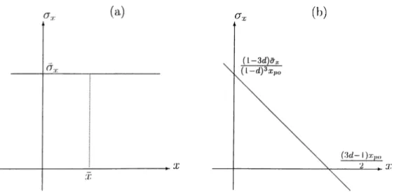
This approximation is more accurate for larger values of Xp„. This is exjKicted since larger Xp„ correspond to less deep perspective projections. The Wigner distribution of the cdiirp given in (6.10) is a line delta given by;

‘2.(7x ( T x j l - 3/t)

(1 - (1 - K.y^Xpo\ ’ 32

( Jt. (b)

Figure 6.2: (a) Wigner distribution of the original exponential, (b) VVigner distribution of the approximate perspective projection: a chirp.

and is shown in Figure C.2b.

Having obtained an approximate analytical form for the perspective projection of a harmonic, as well as its Wigner distribution, we now move on to our discussion of perspective i)rojections in the space-frequency plane, as well as its relation to the fractional Fourier transform.

6.3

P ersp ective

P rojection s

and

Fractional

Fourier Transforms

In the previous section, we obtained an approximate expression for the Wigiuir distribution of the perspective projection of a single exponential. The Wigner distribution of a typical exponential and the Wigner distribution of the approximate perspective projection of the exponential are shown in Figure 6.2. The angle the line delta makes with the x axis is arctan

on &x. The fact that the oblique line delta is a rotatec

2(Jr. _{, which depends} version of the horizontal line delta sugg(;sts a role for the fractional Fourier transform since this operation

corresponds to rotation in the space-frequency plane.

We will now show how the perspective projection of a signal can Ixi approxinmtely (!xi)iessed in terms of the fractional Fourier transform. We claim that the perspective projection of a signal can be obtained from, or mod(ded by, the following steps:

1. Shift the signal by it: in the negative x direction and by a.j., in the luigative fT,; direction. This translates the Wigner distribution of tlui signal to the origin of the spacii-freciuency plane.

2. Tak(i the fractional Fourier transform with the order a = — arctan_7T

angle an/2.

2(Tr.{x+xo)

---^2 ■■ This rotates the Wigner distribution by an

3. Shift th(! result by in the positive x direction and by _XOXpo in the positive (7,; direction.

These steps represent a decomposition of the overall effect of tin; perspective projection, from which we see that the substance of perspective projection is essentially to (iffect a rotation in the space-frequency plane. However, this rotation is enacted on the space-frequency content of the signal referred to tlui origin of the si)ace-frequency plane. The above steps are illustrated in Figure 6.3.

Different iix'.qmmcy components of the signal require differ(uit fractional Fourier orders, l)ecause the order a given in step 3 depends on cf,,.. However, as we will se(g under ciu'tain conditions, a satisfactory approximation can b(i obtained by using a uniform order corresponding to the central fnxiuency of the

We now demonstrate our claim that perspective projection can b(i decomposed into the three steps given above. We start by decomposing f( x) into harmonics:

/(.'/;) = I F{ax)exp{2inxa.j,)da^, 34

a,.. (Jr. G.r. ( J ,:

□

Figure 6.3: Illustration of the decomposition of the approximation into elementaiy ojxirations in the space-frequency plane, a) Original signal. 1)) After step 1 (Space and frequency shift), c) After step 2 (Fractional Fouricir transi()rm.) d) After st(ip 3 (Sj)ace and frequency shift): Approximate perspective projection.

We will concentrate on a single harmonic component exp(z27r.x'(7i:) and the r(!srdt for general f{ x) will follow by linearity. Applying step 1 to a single harmonic we obtain

Qxp{i2nxax). (6.14)

Now, we apply stej) 2 and step 3 to this result to obtain

1/2

i+'i-. 2a,r.'i; -I- .Xq

,v.2 .V.3

Xj)qXq

exp{i2nxax) e x p i2ttx (T2 t- + •'*''0

.^2 (6.15)

Finally, w(! ap[)ly step 4 and obtain our final result: ^ ,2α,.(.x-l·.x„)■’V ^ ' .-o - ^ 1 + *--- 1--- _{,,.2 ,,.3} exp(*27T.X(Jx) e x p '¿27rCTj. ( X — X + ,Xo X + .X,₀ X e x p lA-na. I ,,.2 .,.3 ( x-^-rV xf)Xpa , (6.16) Multiplying this with F{ax) and integrating over yields the ch'sired approximate expriission for the perspective projection of /(.x), which is the mathematical expression of the four steps outlined above.

To see that this expression is indeed an approximation of the perspectivci projection, we again concentrate on a single harmonic component whose exact perspectiv(i projection is e x p 2z7T(7i X()Xp Xpo Xp^ (6.17) 35

Using the, Taylor scuies expansion we obtain exp < i2'Ka.j.Xi) •2 X p j l - 3k) AC" (6.18) { l - K ) ^ X p „ ( l - « ; )3j j ’

which (lifi'ers iVoiii (6.16) only l.)y a constant factor. As far as a single harmonic component is concerned, the only approximation that is involved is the hinomial expansion in the exponent. When the harmonic components are superposed to obtain th(i original function f( x) , we make the additional approxirmition of using the order corresponding to the center frequency for all harmonic components. Thus our three-ste[) procedure will deviate from the exact perspective projection more and more as the bandwidth of f{ x) is increased. The limitations associatcid with this approximation will be discussed in the next section.

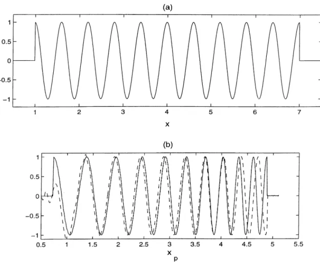
Figure 6.4 shows the exact perspective projection of the function

cos(47ra;)rect X - 4

6

exp(z47ra;) + exp(—z47ra;)

rect X — 4 (6.19)

po

6

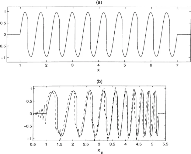
superimposed with the approximation given by (6.18). We chose xq = —3, x as the center of projection. As a second example, we consider the narrowband signal shown in Figure 6.5. Again, the exact perspective projection and the fractional Fourier approximation are superimposed in part b of the same figure. We of)serve that the approximation is quite satisfactory except very near the edges, which shotdd be avoided.

Generalization of the proposed method to two dimensions is possible by following sirniliar steps. In our two-dimensional perspective model we use a two- dimensional image with midpoints x, y\ center frequencies (J,, and spatial widths Ax, Ay. Our center of projection is located at [xQ,Xpo,0). The model described is shown in Figure 6.6.

W ith this model, using simple geometry we can obtain the following mapi)ings and reverse mappings for each Xp and ?/p:

XXr.

Xp -- ^po

X -1- ;co 36

(a)

(b )

Figure 6.4: a.) Original signal, b) Exact perspective projection (solid line)

(a)

Figure 6.5: a.) Original signal, b) Exact perspective projection (solifl line)

Figure 6.6: Perspective model: f{ x,y) represents the object distribution on the x-y plane, g{xp,yp) represents its perspective projection onto the Xp-yp plane. The point A with coordinates (—.xq, OJpo, 0) is the center of projection.

X{)Xp X = --- — Up = •^p.o ‘^p xAy + 2xoy 2[x + xq) (Jp^po y = — X p A y Xpo ^ p ^(^*0 ^p')

As in the one-dirnensional case we first decompose f{ x, y) into harmonics, fix, y) = j F{(Tx, Uy) e-xp[i2TTaxx) Qxp[i2'Kayy) da-x day.

(6.21)

(6.22)

(6.2.3)

(6.24) We proce(!cl by writing an expression for the perspective projection of a two- dimensional harmonic exp[i27rd'j;a:] exp[f27rd’j,7/]:

(ixp i27rarXT.X0 x'^ J'p ^ X p j l - 3k) ^ (1 - K^xlo (1 - K^Xpo (1 - Kf X exp —tTTayAy X p ₊ X p i l — 3 k, ') ₊ K /.'3 X exp i2Tray7jp (1 — k')^Xq (1 — K')^.'ro (1 “ ^0^ ^ X p { \ — 3k) ^ 3Kf — 3 /i 4- 1^ Xt, (6.25) and ^p(l - («·' - 1)·^ .

where again the; binomial approximation has been employed and k =

k' = xf^y ■ Close examination of (6.25) reveals that we have the product of a oiio;-

dimensional chirp in the Xp direction and a scaled harmonic in the; yp direction whose scaling factor depends on Xp. We are going to approximate the perspective projection by using one-dimensional shifts and one-dirnensional fractional Fouri(;r transforms followed by scaling. We claim that the two-dimensional perspective projection of a signal can be obtained from, or modeled by, the following st(;ps:

1. Shift the signal by x in the negative x direction and by dx in the negative Gx direction. This translates the Wigner distribution of the signal to the origin of the space-frequency plane.

2. Take; the one-dimensional fractional Fourier transforms in the variable with order a_ - 2 arctan 2äx(x+xo)'^ _ (x+Ay)^äy_•^po^O^ 2 _Ay'^xl , treating y as a parameter. This rotates the Wigner distributions by an angle air/2.