METHODS FOR TARGET DETECTION IN SAR
IMAGES
a thesis
submitted to the department of electrical and
electronics engineering
and the institute of engineering and science
of b
˙Ilkent university
in partial fulfillment of the requirements
for the degree of
master of science
By
Kaan Duman
December 2009
I certify that I have read this thesis and that in my opinion it is fully adequate, in scope and in quality, as a thesis for the degree of Master of Science.
Prof. Dr. A. Enis C¸ etin(Supervisor)
I certify that I have read this thesis and that in my opinion it is fully adequate, in scope and in quality, as a thesis for the degree of Master of Science.
Prof. Dr. ¨Omer Morg¨ul
I certify that I have read this thesis and that in my opinion it is fully adequate, in scope and in quality, as a thesis for the degree of Master of Science.
Assoc. Prof. Dr. U˘gur G¨ud¨ukbay
Approved for the Institute of Engineering and Science:
Prof. Dr. Mehmet Baray Director of the Institute
ABSTRACT
METHODS FOR TARGET DETECTION IN SAR
IMAGES
Kaan Duman
M.S. in Electrical and Electronics Engineering
Supervisor: Prof. Dr. A. Enis C
¸ etin
December 2009
Automatic recognition and classification of man-made objects in SAR (Syn-thetic Aperture Radar) images have been an active research area because SAR sensors can produce images of scenes in all weather conditions at any time of the day which is not possible with infrared and optical sensors [1, 2]. In this thesis, different feature parameter extraction methods from SAR images are proposed. The new approach is based on region covariance (RC) method which involves the computation of a covariance matrix of a ROI (region of interest). Entries of the covariance matrix are used in target detection. In addition, the use of computationally more efficient region codifference matrix for target detection in SAR images is also introduced. Simulation results of target detection in MSTAR (Moving and Stationary Target Recognition) database are presented. The RC and region codifference methods deliver high detection accuracies and low false alarm rates. The performance of these methods is investigated with various dis-tance metrics and Support Vector Machine (SVM) classifiers. It is also observed that the region codifference method produces better results than the commonly used Principle Component Analysis (PCA) method which is used together with SVM.
The second part of the thesis offers some techniques to decrease the compu-tational cost of the proposed methods. In this approach, ROIs are filtered by directional filters (DFs) at first as a pre-processing stage. Images are categorized according to the filter outputs. The proposed RC and codifference methods are applied within the categories determined by these filters. Simulation results of target detection in MSTAR database are presented through decisions made with l1 norm distance metric and SVM. The number of comparisons made with the
training images using l1 norm distance measure decreases as these images are
distributed into categories. Therefore, the computational cost of the previous algorithm is significantly reduced. SAR image classification results based on l1 norm distance metric are better than the results obtained using SVM and
they show that the two-stage approach does not reduce the performance rate of the previously proposed method much, especially when codifference features are used.
Keywords: Synthetic Aperture Radar (SAR) images, Automatic Target Recog-nition (ATR) and Classification, region covariance (RC), region codifference ma-trix, directional filters (DFs), Support Vector Machines (SVM), Principal Com-ponent Analysis (PCA)
¨
OZET
SAR ˙IMGELER˙INDE HEDEF TESP˙IT Y ¨
ONTEMLER˙I
Kaan Duman
Elektrik ve Elektronik M¨
uhendisli¯gi B¨ol¨
um¨
u Y¨
uksek Lisans
Tez Y¨oneticisi: Prof. Dr. A. Enis C
¸ etin
Aralık 2009
SAR (Sentetik A¸cıklık Radarı) imgelerinde insan yapımı nesnelerin otomatik tanıma ve sınıflandırması aktif bir ara¸stırma alanı olu¸sturmu¸stur, ¸c¨unk¨u kızıl¨otesi ve optik algılayıcıların aksine SAR algılayıcıları g¨un¨un her saatinde ve her t¨url¨u hava ¸sartlarında imge ¨uretebilmektedir [1, 2]. Bu tezde, SAR imgelerinden ¸ce¸sitli ¨oznitelik parametre ¸cıkarma y¨ontemleri sunulmaktadır. Bu yeni yakla¸sım bir ilgi b¨olgesinin (ROI) ortak de˘gi¸sinti matrisinin hesaplanmasını i¸ceren b¨olge or-tak de˘gi¸sinti (RC) y¨ontemine dayanmaktadır. Oror-tak de˘gi¸sinti matrisinin ele-manları hedef tespitinde kullanılmı¸stır. Ayrıca, SAR imgelerinde hedef tespiti i¸cin hesaplama y¨uk¨u a¸cısından daha verimli olan b¨olge ortak fark matrisi de tanıtılmı¸stır. MSTAR (Hareketli ve Dura˘gan Hedef Tanıma) veritabanı ¨
uzerinde hedef tespit benzetim sonu¸cları verilmi¸stir. B¨olge ortak de˘gi¸sinti ve fark y¨ontemleri y¨uksek tespit do˘grulukları ve d¨u¸s¨uk yanlı¸s kabul y¨uzdeleri or-taya koymaktadır. Bu y¨ontemlerin performansları ¸ce¸sitli uzaklık metrikleri ve Destek¸ci Vekt¨or Makine (SVM) sınıflandırıcıları kullanılarak incelenmi¸stir. Aynı zamanda, benzetim sonu¸clarına bakıldı˘gında, b¨olge ortak fark y¨onteminin yaygın olarak uygulanan ve burada SVM ile birlikte kullanılan Temel Bile¸senler Analizi (PCA) y¨ontemine g¨ore daha iyi sonu¸clar verdi˘gi g¨ozlemlenmi¸stir.
Tezin ikinci b¨ol¨um¨unde, ¨onerilen y¨ontemlerin hesaplama y¨uk¨un¨u azaltmak i¸cin yeni teknikler ¨one s¨ur¨ulmektedir. Bu yakla¸sımda, bir ¨oni¸sleme kademesi olarak imge b¨olgeleri y¨on s¨uzge¸clerinden (DFs) ge¸cirilmi¸stir. Onerilen or-¨ tak de˘gi¸sinti ve fark y¨ontemleri, bu s¨uzge¸cler aracılı˘gıyla belirlenen kategoriler i¸cerisinde uygulanmı¸stır. MSTAR veritabanında l1d¨uzge uzaklık metri˘gi ve SVM
kullanılarak alınan kararlar do˘grultusunda hedef tespit benzetim sonu¸cları or-taya konulmu¸stur. E˘gitim imgelerinin kategorilere ayrılmasından dolayı, l1 d¨uzge
uzaklık ¨ol¸c¨ut¨u kullanıldı˘gında bu imgelerle yapılan kar¸sıla¸stırma sayısı azalmak-tadır. Bu sayede, ¨onceki algoritmanın hesaplama y¨uk¨u b¨uy¨uk ¨ol¸c¨ude d¨u¸ser. Uzaklık ¨ol¸c¨ut¨u olarak l1 d¨uzgeye dayalı SAR imge sınıflandırması sonu¸cları SVM
kullanılarak elde edilen sonu¸clara g¨ore daha iyidir. Ayrıca bu sonu¸clar, ¨ozellikle ortak fark ¨oznitelikleri kullanıldı˘gında, iki-kademeli sistemin hedef tespit perfor-mansının ¨onerilen ¨onceki y¨onteme g¨ore fazla d¨u¸smedi˘gini g¨ostermi¸stir.
Anahtar Kelimeler: Sentetik A¸cıklık Radarı (SAR) imgeleri, Otomatik Hedef Tanıma (ATR) ve Sınıflandırması, b¨olge ortak de˘gi¸sinti (RC), b¨olge ortak fark matrisi, y¨on s¨uzge¸cleri (DFs), Destek¸ci Vekt¨or Makineleri (SVM), Temel Bile¸senler Analizi (PCA)
ACKNOWLEDGMENTS
I would like to express my gratitude to Prof. Dr. A. Enis C¸ etin for his su-pervision, suggestions and encouragement throughout the development of this thesis.
I am also indepted to Prof. Dr. ¨Omer Morg¨ul and Assoc. Prof. Dr. U˘gur G¨ud¨ukbay for accepting to read and review this thesis.
I wish to thank my family, my friends and my colleagues at our department for their support and collaboration.
I would also like to thank T ¨UB˙ITAK for funding the work presented in this thesis with M˙ILDAR Project (No. 107A011).
Contents
1 Introduction 1
1.2 Feature extraction from SAR images . . . 3 1.3 Thesis Outline . . . 4
2 Target Detection in SAR Images Using Region Covariance (RC)
and Codifference 6
2.1 Related Work on Region Covariance (RC) Method . . . 8 2.2 Region Covariance (RC) Matrix . . . 9 2.3 Region Codifference Matrix . . . 11 2.4 The Moving and Stationary Target Recognition SAR Database . . 12 2.5 Stages of the Target Detection Algorithm . . . 15 2.6 Simulation Results . . . 18
2.6.1 Using Various Distance Metrics and Support Vector Ma-chine (SVM) Classifiers . . . 19 2.6.2 Using Principal Component Analysis (PCA) Method . . . 28
2.7 Summary . . . 31
3 Use of Directional Filters (DFs) on Target Detection Methods 32 3.1 Introduction . . . 32
3.2 Pre-processing Stage and Directional Filter (DF) Design . . . 34
3.3 Target Detection Strategy . . . 37
3.4 Simulation Results . . . 38
3.4.1 Using k-Nearest Neighbor (k-NN) Algorithm . . . 51
3.5 Summary . . . 54
List of Figures
1.1 Synthetic aperture radar (SAR) working principle (adopted from [3]). . . 2 1.2 Block diagram of a typical SAR ATR (Automatic Target
Recog-nition) system. . . 3
2.1 Block diagram of three-stage baseline SAR ATR system proposed by Novak et al. [4]. . . 8 2.2 DHC-6 Twin Otter Aircraft which carries Sandia National
Labo-ratories Twin Otter SAR sensor (adopted from [3]). . . 13 2.3 A sample for X band SAR image collected in DARPA Moving and
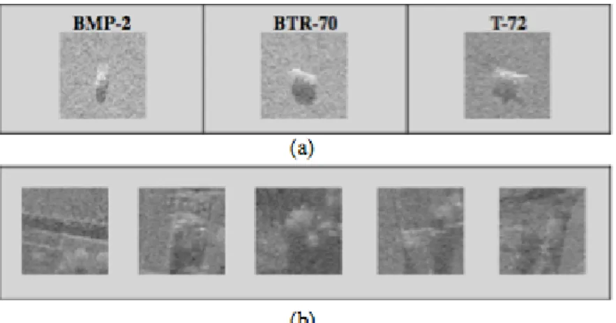
Stationary Target Recognition (MSTAR) program. . . 13 2.4 Targets in the MSTAR: (a) BMP-2 Armored Personal Carrier, (b)
BTR-70 Armored Personal Carrier, (c) T-72 Main Battle Tank [5]. 14 2.5 Several target and clutter images: (a) Target images of size
128-by-128, (b) Clutter images of size 128-by-128. . . 15 2.6 Block diagram showing stages of the target detection algorithm. . 16 2.7 A sample covariance or codifference matrix where the bounded
2.8 Examples of 128-by-128 and 64-by-64 target and clutter images (ROIs). 64-by-64 images are cropped from the 128-by-128 images. 18 2.9 The target detection accuracies (%) obtained with various decision
techniques using (a) RC and (b) codifference methods proposed. . 24 2.10 The false alarm rates (%) obtained with various decision
tech-niques using (a) RC and (b) codifference methods proposed. . . . 25 2.11 The target detection accuracies (%) obtained for increasing k
val-ues using l1 norm distance metric. . . 27
2.12 The false alarm rates (%) obtained for increasing k values using l1 norm distance metric. . . 27
3.1 Block diagram of the two-stage target detection process investi-gated in this chapter . . . 33 3.2 Design of the directional filters (DFs) . . . 35 3.3 Block diagram of the pre-processing stage . . . 36 3.4 Block diagram of the target detection stage applied in each
cate-gory using (a) l1 norm distance metric in Eq. 3.1 (b) SVM classifiers. 38
3.5 Example 64-by-64 target images selected by DFs 1 - 10 . . . 39 3.6 (a) Target detection accuracies (%) and (b) false alarm rates (%)
obtained with the two-stage methods working on 10 categories . . 41 3.7 (a) Target detection accuracies (%) and (b) false alarm rates (%)
obtained with the two-stage methods working on 8 categories . . . 42 3.8 (a) Target detection accuracies (%) and (b) false alarm rates (%)
3.9 (a) Target detection accuracies (%) and (b) false alarm rates (%) obtained with the two-stage methods working on 6 categories . . . 44 3.10 (a) Target detection accuracies (%) and (b) false alarm rates (%)
obtained with the two-stage methods working on 5 categories . . . 45 3.11 (a) Target detection accuracies (%) and (b) false alarm rates (%)
obtained with the two-stage methods working on 4 categories . . . 47 3.12 (a) Target detection accuracies (%) and (b) false alarm rates (%)
obtained with the two-stage methods working on 3 categories . . . 48 3.13 (a) Target detection accuracies (%) and (b) false alarm rates (%)
obtained with the two-stage methods working on 2 categories . . . 49 3.14 The total target detection accuracies (%) obtained with the
two-stage RC and codifference methods using various decision tech-niques on different numbers of categories . . . 50 3.15 The total false alarm rates (%) obtained with the two-stage RC
and codifference methods using various decision techniques on dif-ferent numbers of categories . . . 50 3.16 (a) Target detection accuracies (%) and (b) false alarm rates (%)
obtained with the two-stage methods working on 10 categories of the new database . . . 52 3.17 The total target detection accuracies (%) obtained for increasing
k values on 10 categories for the two-stage system using l1 norm
distance metric. . . 53 3.18 The total false alarm rates (%) obtained for increasing k values
on 10 categories for the two-stage system using l1 norm distance
List of Tables
2.1 Number of images used in training and testing studies . . . 19 2.2 Target detection accuracies and false alarm rates achieved using
RC and region codifference methods with the distance metric de-fined in Eq. 2.7 . . . 20 2.3 Target detection accuracies and false alarm rates achieved using
RC and region codifference methods with the distance metric de-fined in Eq. 2.8 . . . 20 2.4 Target detection accuracies and false alarm rates achieved using
RC and region codifference methods with the distance metric de-fined in Eq. 2.9 . . . 21 2.5 Target detection accuracies and false alarm rates achieved using
RC and region codifference methods with the distance metric de-fined in Eq. 2.10 . . . 22 2.6 Target detection accuracies and false alarm rates achieved using
RC and region codifference methods with the distance metric de-fined in Eq. 2.11 . . . 22 2.7 Target detection accuracies and false alarm rates achieved using
2.8 The target detection accuracies and false alarm rates obtained with various numbers of training images . . . 26 2.9 Number of images used in training and testing studies for the PCA
method . . . 29 2.10 Target detection accuracies and false alarm rates achieved using
PCA method . . . 29 2.11 Target detection accuracies and false alarm rates achieved using
the distance metric defined in Eq. 2.9 . . . 30 2.12 Target detection accuracies and false alarm rates achieved using
SVM as a classifier . . . 30
3.1 Number of training and test images used for the two-stage methods working on 10 categories . . . 40 3.2 Number of training and test images used for the two-stage methods
working on 8 categories . . . 42 3.3 Number of training and test images used for the two-stage methods
working on 7 categories . . . 43 3.4 Number of training and test images used for the two-stage methods
working on 6 categories . . . 44 3.5 Number of training and test images used for the two-stage methods
working on 5 categories . . . 45 3.6 Number of training and test images used for the two-stage methods
3.7 Number of training and test images used for the two-stage methods working on 3 categories . . . 47 3.8 Number of training and test images used for the two-stage methods
working on 2 categories . . . 48 3.9 The total target detection accuracies and false alarm rates
ob-tained with various numbers of training images on 10 categories . 51 3.10 Number of training and test images used for the two-stage methods
Chapter 1
Introduction
Synthetic Aperture Radar (SAR) sensors can produce images of scenes in all weather conditions at any time of day and night which is not possible with infrared or optical sensors. Another useful feature of SARs is the geometric res-olution that does not depend upon the operating frequency. Because of these reasons, automatic recognition and classification of man-made (metal) objects in SAR images have been an active research area in recent years [1, 2]. There are many application areas in which the recognition of a target or texture sig-nal is important in SAR images. Besides target detection and classification for military purposes, applications of SAR include recognition of the terrain sur-face for mineral exploration, determining the spilled oil boundaries in oceans for environmentalists and extracting the sea state and ice hazard maps for naviga-tors. Furthermore, the number of applications can be increased in other areas including military combat identification, meteorological observation, battlefield surveillance, mining, oceanography, classification of earth terrain etc. [2].
SAR images are typically two dimensional (2-D) images. A SAR image per-pendicular to the aircraft’s direction is constructed as in the following Fig. 1.1 adopted from [3]. The first dimension is called range (or cross track), which is
a measure for the line-of-sight distance of the target to the aircraft. Similar to most radars, the range is determined by measuring the time between the trans-mitted pulse and its echo. A narrow pulse width leads to a high resolution in range. The other dimension is named as azimuth, which is along the track of the aircraft. To have fine azimuth resolution, a physically large antenna is needed, which is impossible to be deployed on an aircraft. Instead, to produce the data of a large antenna, pieces of data are collected and processed as the aircraft flies along its track in a certain distance called synthetic aperture distance.
Figure 1.1: Synthetic aperture radar (SAR) working principle (adopted from [3]).
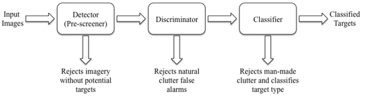
There are numerous advantages of the SAR system as described above. These advantages make target detection and classification in SAR images specifically vi-tal. Many SAR Automatic Target Recognition (ATR) algorithms were developed in the literature [6] -[11]. As shown in Fig. 1.2, a complete ATR system includes five stages: detection, discrimination, classification, recognition, and identifica-tion. In many systems, only some of the above stages are available. Therefore,
Figure 1.2: Block diagram of a typical SAR ATR (Automatic Target Recognition) system.
a typical SAR ATR system fulfils three functions: detection (pre-screener), dis-crimination and classification as will be discussed in Chapter 2. The contribution of this thesis is in the area of detection (pre-screener) or discrimination stage of the SAR ATR.
1.2
Feature extraction from SAR images
Porikli and Tuzel used the region covariance (RC) method to describe an image region using the covariance matrix in order to extract features for detection and classification problems. The RC approach provides robustness on the images in terms of orientation and illumination changes to a certain degree. Moreover, the dimensionality of the covariance matrix does not change with the size of the input image region. In recent years, region covariance is successfully used in face, human, license plate, various objects and texture detection and classification problems in still images and video [12, 13, 14, 15].
In this thesis, the RC and the codifference matrix methods are used in SAR ATR target detection problem. Feature parameters of the region of interests (ROIs) in the images are extracted using the RC method proposed by Porikli et al. The goal is to describe an image region with a covariance matrix for detection of man-made objects in SAR images. The computational cost of the RC method is reduced by introducing a new matrix called codifference matrix which can be used instead of the RC matrix. Various distance metrics are introduced along with the one used in [12] to match the closest regions within the search space of
images. Support Vector Machines (SVMs), which implement Euclidean distance as parameter of measure, are also used as a part of the decision strategy. In real-time applications, SVM classifiers provide the least computational complexity. Simulation results are presented by comparing the proposed approaches to a former method using Principal Component Analysis (PCA) with SVM.
In our work, SAR images are pre-processed with directional filters before the RC and the codifference algorithm. This approach makes it possible to classify ROIs in the training stage into various categories, which results in a reduction on the number of training images to be compared. Therefore, the computational cost of the algorithm significantly decreases as distances between test and the training feature vectors are determined by one-to-one matching between these vectors through l1 norms. Same principle is not valid for the decisions made
with SVM, as total number of images trained stays equal with the old methods. Still the results obtained by SVMs are presented for comparing SVMs’ detection performances to the methods using l1 norm based distance metric.
All simulations are carried out using the images of the MSTAR (Moving and Stationary Target Recognition) SAR database [16], which is the only publicly available database. The database includes the images of various types of fields and targets which include armed personal carriers and a tank made by the Former Soviet Union. Simulation results are presented at the end of each chapter.
1.3
Thesis Outline
The rest of this thesis is organized as follows. In Chapter 2, the RC and region codifference target detection methods are stated and simulation results with dif-ferent distance measures are given with comparisons to SVM and PCA methods. Chapter 3 introduces the use of directional filters as a pre-processor to the RC and region codifference method with simulation results on decisions made using
l1 norm distance metric and SVM classifiers. Conclusions are made and a list of
Chapter 2
Target Detection in SAR Images
Using Region Covariance (RC)
and Codifference
In this chapter, the use of region covariance (RC) and codifference matrices in order to detect targets in SAR (Synthetic Aperture Radar) images is described. These matrices form the features of the region of interests (ROIs) extracted from the target and clutter images. Distances between the features of test and training images are calculated with different metrics to be introduced. In addition, SVMs (Support Vector Machines) are used to detect targets in the SAR images.
The images used in this thesis are obtained from the only publicly avali-able SAR database: MSTAR (Moving and Stationary Target Recognition) database [16]. The contents of this database can be found in Section 2.4. The images are divided into training and test datasets. The test image features are matched to target or clutter train image features using different distance metrics based on generalized or distinct eigenvalues and l1 norms with and without
the decisions made with l1 norm distance metric. Furthermore, SVMs are used
to train and test the covariance and codifference features. Simulation results are compared with a PCA (Principal Component Analysis) based method which is also using SVM. The results include target detection accuracies and false alarm (incorrectly classified clutter images) rates. Simulations to obtain the results were carried out using a MATLAB computing environment (version R2009b).
The region covariance method was first introduced by Porikli et al. The related work on this method is briefly discussed in Section 2.1. The codifference matrix, developed over the cause of this thesis, is defined by modifying the RC matrix and has lower computational cost.
The RC and codifference approach investigated in this chapter can be used in the detection and discrimination stages of a SAR ATR system. Target detection and discrimination are the first stages of a typical SAR ATR system. These stages are important in improving the whole ATR system’s performance. In Fig. 2.1 adopted from the works of Novak et al. [4], one can see both target detection and discrimination process forming the first two stages of the three-stage baseline SAR ATR system. Images without potential targets and natural clutter false alarms are rejected in these stages. There are many target detection and discrimination algorithms for SAR images described in the literature [6] -[10]. CFAR (constant false alarm rate) method is generally used for target detection. It uses the amplitude information and discards the phase of the SAR images, which involves excess data [4, 5, 17].
Figure 2.1: Block diagram of three-stage baseline SAR ATR system proposed by Novak et al. [4].
The remaining parts of this chapter are organized as follows. The related work in literature on Porikli’s RC method is presented in Section 2.1. RC and codifference matrices are presented in detail in Sections 2.2 and 2.3. The MSTAR database is overviewed in Section 2.4 and the target detection stages are revealed in Section 2.5. Finally, simulation results on the MSTAR SAR database are delivered in Section 2.6.
2.1
Related Work on Region Covariance (RC)
Method
The region covariance (RC) method describes an image region with a covariance matrix in order to extract features for image detection and classification prob-lems. In recent years, this method is successfully used in face, human, license plate and different objects detection and classification problems [12, 13, 14].
Given a ROI where the object to be detected is searched, one or more co-variance matrices are computed for cropped chips of the ROI in different size. The covariance features are fed to a multi-layer neural network [14] or Logit-Boost classifiers [13]. Besides learning mechanisms, a distance metric involving
computation of generalized eigenvalues is used in order to match the covariance descriptors [12]. The RC method is also adapted to object tracking applications in video, where the object is described using the covariance matrix [15]. In a frame, the object is found in the ROI where the minimum distance between the RC matrix of the model object and the ROI is achieved. From frame to frame, the variations are adapted by keeping a set of previous RC matrices and extract-ing a mean on the Riemannian manifolds. The system is shown to be accurately detecting non-rigid, moving objects in non-stationary camera sequences while achieving a detection rate of 97.4% in [15].
In this work, the RC method is applied to SAR images to detect man-made (metal) objects. The distance metric based on the generalized eigenvalues in [12] is used besides other metrics in matching the matrix features extracted from the training and test images.
2.2
Region Covariance (RC) Matrix
In this section, the region covariance (RC) as an image region descriptor is pre-sented. In ROIs of the target and clutter images in the MSTAR database, RC matrix is used to extract feature parameters.
To detect targets on SAR images, one RC matrix is extracted for a ROI. It is assumed that features obtained from a single covariance matrix are enough to discriminate between distributions, which results in minimum computational cost for the algorithm. For each pixel in the ROI, a seven-dimensional feature vector z is computed as,
zk =
!
x y I(x, y) dI(x,y)dx dI(x,y)dy d2I(x,y)dx2
d2I(x,y)
dy2
"
(2.1) where, k is the label of a pixel, (x, y) is the position of a pixel, I is intensity of a pixel (as gray scale images are used in this work), dI(x, y)/dx is the horizontal
and dI(x, y)/dy is the vertical derivative of the ROI calculated through the filter [−1 0 1] , d2I(x, y)/dx2 is the horizontal and d2I(x, y)/dy2is the vertical second derivative of the ROI calculated through the filter [−1 2 − 1] . For a 4 by 4 region, k = 1, 2, ...16; x =−2, 1, 0, 1. One should note that in filtering processes, there is no need for computationally costly multiplications, as the result can be found out by addition and subtraction of the shifted sequences of input data.
Different items could be added to the feature vector z as in [13]. Again, let the feature vector z be defined as:
zk = [zk(i)]T (2.2)
where i is the index of the feature vector. After obtaining this vector, a fast method for computing the RC matrices by using integral images is applied. This method has the same calculation complexity for all window sizes after computing the integral images as provided in [18]. The 7-by-7 covariance matrix CR of a
ROI R is defined by the fast covariance matrix computation formula: CR = [cR(i, j)] = # 1 n− 1 $ n % k=1 (zk(i)zk(j))− 1 n n % k=1 zk(i) n % k=1 zk(j) &' (2.3) where n is the total number of pixels in the ROI and cR(i, j) is the (i, j)th
component of the covariance matrix.
There are several advantages of using covariance features to describe a ROI. First, these features have small dimension and they are invariant to a degree of scale and illumination change as these characteristics are all absorbed within the covariance matrix. For instance, given a ROI, its covariance CR does not have
any information regarding the number of pixels, because size of the CR is due
to the number of items in feature vector z, not to the number of pixels in the ROI. By providing CR as a feature, we look to the relations between the pixels,
which absorb certain illumination changes from image to image. In addition, the computation of covariance intrinsically provides an averaging filter to filter out the natural occurring speckle noise that corrupts SAR images.
2.3
Region Codifference Matrix
In this section, a new region codifference matrix is introduced for target detection which replaces the covariance matrix in the novel RC method.
Computational cost of a single covariance matrix is not heavy. However, computational cost becomes important when scanning large regions at different scales and locations. Furthermore, many video processing applications require real-time solutions. In order to decrease the computational cost, the RC matrix definition in Eq. 2.3 is modified to obtain the codifference equation as in Eq. 2.4.
CR= [cR(i, j)] = # 1 n− 1 $ n % k=1 (zk(i)⊕ zk(j))− 1 n n % k=1 zk(i)⊕ n % k=1 zk(j) &' (2.4) where the scalar multiplication is replaced by an additive operator ⊕. The op-erator ⊕ is basically a summation operation but the sign of the results behaves similar to the multiplication operation.
a⊕ b = a + b if a≥ 0 and b ≥ 0 a− b if a≤ 0 and b ≥ 0 −a + b if a≥ 0 and b ≤ 0 −a − b if a≤ 0 and b ≤ 0 (2.5)
for real numbers a and b. Above equation can be expressed also as follows: a⊕ b = sign(a × b)(|a| + |b|) (2.6) Since a⊕ b = b ⊕ a, the codifference matrix is also symmetric like the RC ma-trix. The codifference matrix behaves similar to the covariance mama-trix. For two variables, the sign of the result for the operations in covariance and codifference is the same. If two variables’ signs are the same, the output is positive and if they are not, the output is negative. In many computer systems, addition is less costly compared to multiplication. This makes the calculation of the codifference matrix computationally efficient compared to the covariance matrix.
The operator⊕ satisfies totality, associativity and identity properties; there-fore it is a monoid function. In other words it is a semigroup with identity property. Similar statistical methods are used in [19]. Another similar statis-tical function is the Average Magnitude Difference Function (AMDF), which is widely used in speech processing to determine periodicity of voiced sounds.
2.4
The Moving and Stationary Target
Recog-nition SAR Database
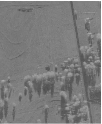
The MSTAR (Moving and Stationary Target Recognition) data was collected using the Sandia National Laboratories Twin Otter SAR sensor payload oper-ating at X band (10 GHz). DHC-6 Twin Otter Aircraft which carries this SAR sensor is shown in Fig. 2.2 [3]. This data was collected and distributed under the DARPA (Defense Advanced Research Projects Agency) MSTAR program. One of the full size X band SAR image collected in this program is shown in Fig. 2.3. The images have 0.3m x 0.3m resolution. All SAR images are acquired at angle of depressions of 15◦ and 17◦. Besides, target images are available in all orientations in the database, i.e. the shots are made over 360◦ target aspect. In
this thesis, all images are treated in an equal manner and all target and clutter images are divided into training and test datasets.
Figure 2.2: DHC-6 Twin Otter Aircraft which carries Sandia National Labora-tories Twin Otter SAR sensor (adopted from [3]).
Figure 2.3: A sample for X band SAR image collected in DARPA Moving and Stationary Target Recognition (MSTAR) program.
MSTAR SAR database used in this thesis is the only publicly available database for SAR imagery. However, obtaining the database still requires a formal registration. The database includes images of targets and clutter. Target images consist of the images of armored personnel carriers BMP-2, BTR-70 and T-72 main battle tank of Former Soviet Union. Images of open fields, farms,
trees, roads and buildings form the clutter images. Therefore there is natural and also cultural clutter in the images. The database contains images of three different vehicles for BMP-2 and T-72, however one for BTR-70. The pictures of these vehicles adopted from [5] are presented in Fig. 2.4. Several target and clutter SAR images in the MSTAR database are provided in Fig. 2.5. A total of 1285 BMP-2, 429 BTR-70 and 1045 T-72 images are available in the database The target images are originally provided in 128-by-128 pixel size chips. The clutter images are cropped in this size randomly from the original 1476-by-1784 sized images (one is shown in Fig. 2.3).
Figure 2.4: Targets in the MSTAR: (a) BMP-2 Armored Personal Carrier, (b) BTR-70 Armored Personal Carrier, (c) T-72 Main Battle Tank [5].
Figure 2.5: Several target and clutter images: (a) Target images of size 128-by-128, (b) Clutter images of size 128-by-128.
2.5
Stages of the Target Detection Algorithm
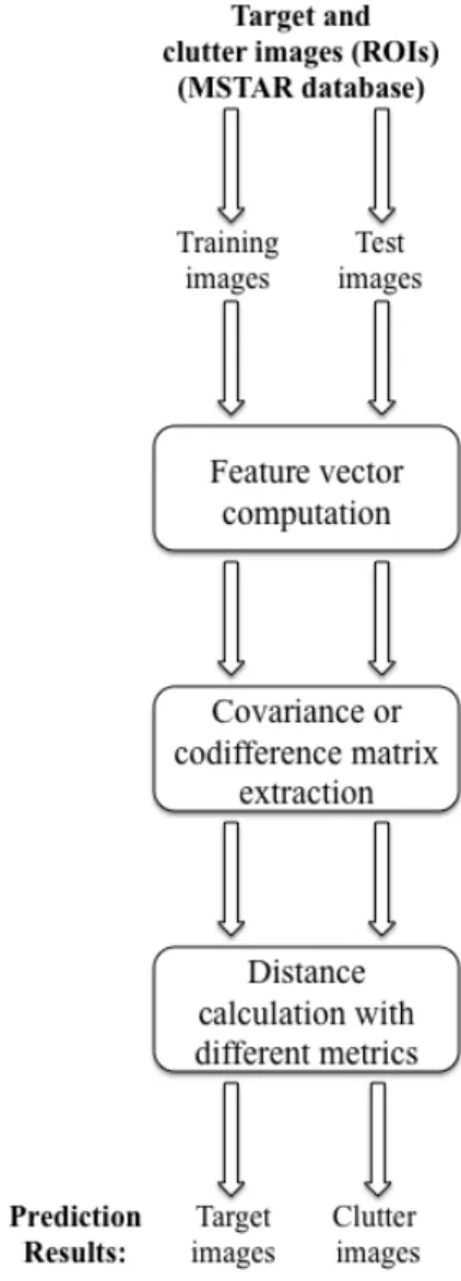
As mentioned earlier, to detect a target, covariance and codifference matrices of target/clutter training and test images are compared to each other using dis-tance metrics providing robust detection and classification. The block diagram of the entire target detection process is illustrated in Fig. 2.6. First, the ROIs of the images in the database (shown in Fig. 2.8) are divided in two datasets as training and test images . Then, as given in Eq. 2.1, the feature vectors of these images are computed for each pixel. The covariance or codifference matrix of the ROIs using these feature vectors is extracted according to Equations 2.3 and 2.4. The distance between the training and test images are found using various distance metrics on vectors of covariance and codifference features. The label (target/clutter) of training image’s ROI producing the smallest distance value determines whether a test image is classified as target or clutter. Thus, target and clutter images of the test dataset are predicted by this way. The covariance and codifference features of training images are also put into SVMs (Support
Vector Machines) and the SVM classifiers are used as a last stage for the target detection algorithm. The results are presented in Section 2.6.1.
Figure 2.6: Block diagram showing stages of the target detection algorithm.
There is no need to use the entire covariance or codifference matrix as input parameters (features) to the decision mechanism. Let the matrix CR in Fig. 2.7
illustrate a covariance or a codifference matrix of a ROI. This matrix is symmet-ric, and therefore the lower (or upper) triangle of the matrix carries the sufficient information for the entire matrix. Moreover, cR(1, 1), cR(2, 1) and cR(2, 2) are
eliminated as these are computed from the (x, y) positions in the feature vector z and are equal in every covariance and codifference matrices, as only one matrix
is extracted from each image. As a result, the necessary covariance or codiffer-ence features shrink only to the bounded components providing a decrease in computational cost of the decision stage.
Figure 2.7: A sample covariance or codifference matrix where the bounded region shows the necessary features for the decision algorithm.
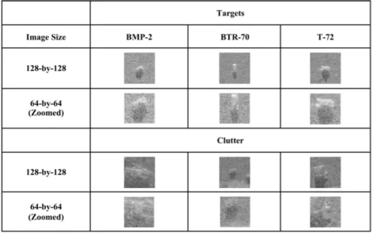
The original target and cropped clutter images of size 128-by-128 pixels and 64-by-64 image chips cut from the original images form the ROIs. The cropped image chips are chosen by inspection, such that the targets are cap-tured as demonstrated in Fig. 2.8. If the original image is depicted by I, I(45 : 108, 33 : 96) represent the 64-by-64 image chip cropped. These chips provide data size reduction during the feature extraction phase, where horizon-tal and vertical filtering is used.
Figure 2.8: Examples of 128-by-128 and 64-by-64 target and clutter images (ROIs). 64-by-64 images are cropped from the 128-by-128 images.
2.6
Simulation Results
Simulation results of the target detection algorithm using RC and codifference methods are presented. In Section 2.6.1, target detection results on covariance and codifference features obtained through various distance metrics and SVM classifiers are delivered. For comparison, SAR image classification results by a former method using PCA (defined in [20]) with SVM are given in Section 2.6.2. The performance of the detection algorithms is determined according to two parameters: (i) detection accuracy = (number of correctly detected target im-ages)/(number of total target test images), (ii) false alarm = (number of clutter images detected as target images)/(number of total clutter test images).
2.6.1
Using Various Distance Metrics and Support Vector
Machine (SVM) Classifiers
The number of target and clutter images divided into training and test datasets used in the simulations are presented in Table 2.1. The relation between number of test images and the number of training images is about 20:1, when target images are considered. The ratio rises up to 100:1, when we focus on the clutter images. These high ratios increase the importance of getting accurate target de-tection and low false alarm rates. Simulation results for whole and target focused 64-by-64 images (ROIs) for the RC and codifference methods using different dis-tance metrics and SVM classifiers are summarized in Tables 2.2, 2.3, 2.4, 2.5, 2.6 and 2.7 in exact ratio and percentages form.
Table 2.1: Number of images used in training and testing studies Number of train images Number of test images
Target 132 2627
Clutter 132 13346
The original distance metric to be used with the RC method is presented by Porikli et. al. [12]. In order to match two ROIs, the calculated covariance matri-ces are compared to each other using this distance metric based on generalized eigenvalues. Two images (or two ROIs R1 and R2) have a distance ρ1 calculated
with their covariance matrices using Eq. 2.7. ρ1(C1, C2) = / 0 0 1 p % i=1 log2(λ i(C1, C2)) (2.7)
Target detection and false alarm rates by using the distance metric in Eq. 2.7 on covariance and codifference matrices are given in Table 2.2.
The studies with the database are expanded such that new distance metrics are defined for comparison of the region covariance and codifference matrices in order to improve the target detection performance. The first modified distance
Table 2.2: Target detection accuracies and false alarm rates achieved using RC and region codifference methods with the distance metric defined in Eq. 2.7
Input images Rates (ROIs)
Target detection False alarm accuracies
Using RC 128-by-128 2625/2627 (99.92%) 86/13346 (0.64%) method 64-by-64 2627/2627 (100%) 1/13346 (∼0%) Using region 128-by-128 2626/2627 (99.96%) 0/13346 (0%) codifference method 64-by-64 2624/2627 (99.88%) 20/13346 (0.15%)
metric ρ2 is defined as the square root of the sum of the logarithmic square of
the differences between respective eigenvalues of C1 and C2 as in Eq. 2.8.
ρ2(C1, C2) = / 0 0 1 p % i=1 log2(λ i(C1)− λi(C2)) (2.8)
where, C1, C2 are the covariance matrices of regions R1 and R2, respectively
and λi is the ith eigenvalue of C1, C2 separately and p(= 7) is the number of
eigenvalues for C1 and C2. The resulting performance rates using this distance
metric are depicted in Table 2.3.
Table 2.3: Target detection accuracies and false alarm rates achieved using RC and region codifference methods with the distance metric defined in Eq. 2.8
Input images Rates (ROIs)
Target detection False alarm accuracies
Using RC 128-by-128 2576/2627 (98.06%) 44/13346 (0.33%) method 64-by-64 2576/2627 (98.06%) 14/13346 (0.1%) Using region 128-by-128 2567/2627 (97.72%) 40/13346 (0.3%) codifference method 64-by-64 2575/2627 (98.02%) 66/13346 (0.49%)
A new distance metric is also defined which is based on the l1 norm distance
calculation rather than eigenvalues on two RC or codifference matrices’ feature vectors. This distance metric is defined as
ρ3(C1, C2) = p % i=1 $ p % j=1 (|C1(i, j)− C2(i, j)|) & (2.9)
where, C1, C2 are the covariance matrices of regions R1 and R2, respectively.
Extracting no eigenvalues and only computing the sum of difference between the training and test covariance and codifference matrix feature vectors significantly reduces the computational cost. The target detection results of SAR images using this distance metric with RC and codifference matrices are shown in Table 2.4. Table 2.4: Target detection accuracies and false alarm rates achieved using RC and region codifference methods with the distance metric defined in Eq. 2.9
Input images Rates (ROIs)
Target detection False alarm accuracies
Using RC 128-by-128 2618/2627 (99.66%) 0/13346 (0%) method 64-by-64 2626/2627 (99.96%) 1/13346 (∼0%) Using region 128-by-128 2627/2627 (100%) 0/13346 (0%) codifference method 64-by-64 2626/2627 (99.96%) 1/13346 (∼0%)
Further, a new distance metric is introduced which finds distance between two ROIs according to the normalization by the diagonal values of covariance or codifference matrices of only the training regions. Since the pixel intensity values and their derivatives in the feature vector z in Eq. 2.1 have different scales of values, normalization is applied while comparing the covariance and codifference matrices of the two regions computed from them. This metric is given as
ρ4(C1, C2) = p % i=1 $ p % j=1 2 |C1(i, j)− C2(i, j)| C2(i, i) 3& (2.10) where, C1, C2 are the covariance matrices of two ROIs R1 and R2, respectively.
For this case, R1 is the region acquired from the test images, whereas R2 is the
region acquired from the training images. The target detection results obtained by applying this distance metric are shown in Table 2.5.
The metric in Eq. 2.10 is also modified such that the normalization is made by contribution of both training and test images’ covariance or codifference matrices. This metric is defined as
ρ5(C1, C2) = p
%$%p 2
|C1(i, j)− C2(i, j)|
(C (i, i) + C (i, i)) 3&
Table 2.5: Target detection accuracies and false alarm rates achieved using RC and region codifference methods with the distance metric defined in Eq. 2.10
Input images Rates (ROIs)
Target detection False alarm accuracies
Using RC 128-by-128 2625/2627 (99.92%) 13/13346 (0.10%) method 64-by-64 2627/2627 (100%) 3/13346 (0.02%) Using region 128-by-128 2627/2627 (100%) 1/13346 (∼0%) codifference method 64-by-64 2626/2627 (99.96%) 0/13346 (0%)
where, C1, C2 are the covariance matrices of regions R1(from test images) and
R2(from training images), respectively. The normalization is done again by the
diagonal values of the covariance or codifference matrices. The resulting target detection performances using this metric are given in Table 2.6
Table 2.6: Target detection accuracies and false alarm rates achieved using RC and region codifference methods with the distance metric defined in Eq. 2.11
Input images Rates (ROIs)
Target detection False alarm accuracies
Using RC 128-by-128 2625/2627 (99.92%) 4/13346 (0.03%) method 64-by-64 2627/2627 (100%) 1/13346 (∼0%) Using region 128-by-128 2626/2627 (99.96%) 0/13346 (0%) codifference method 64-by-64 2626/2627 (99.96%) 0/13346 (0%)
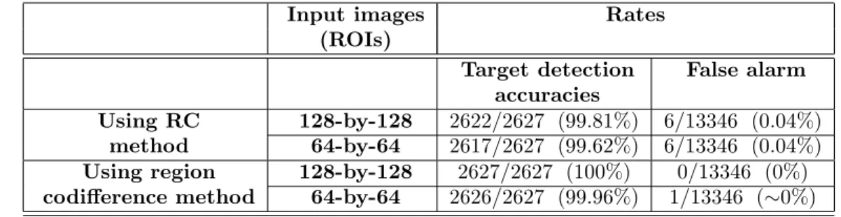
Finally, SVMs are used in order to distinguish between the covariance or codifference feature vectors extracted from the training and test images to detect targets/clutter in the database. SVM is a supervised machine learning method based on the statistical learning theory and approach developed by Vladimir Vapnik. SVMs have been applied to SAR target classification problems and they exhibit superior performance measures compared to other classifiers [9]. There are many parameters corresponding to different SVM kernels. In this study, the polynomial SVM kernel proposed in [21] is chosen, although, the RBF (Radial Basis Function) and linear SVM kernels are also implemented. It is observed
that when RBF kernel is used on the RC features, it fails to classify almost half of the target and clutter test images into any decision group. This kernel also returns high false alarm rates, when it is used with the region codifference method. Therefore, the RBF kernel does not provide any good results unlike the polynomial kernel. The overall classification performance also decreases when linear kernel is used. As a result, among the three kernels, the polynomial kernel gives the best performance rate for the SAR target detection problem investigated in this thesis. Thus, the results acquired through SVM with polynomial kernel are given in Table 2.7
Table 2.7: Target detection accuracies and false alarm rates achieved using SVM as a classifier
Input images Rates (ROIs)
Target detection False alarm accuracies
Using RC 128-by-128 2622/2627 (99.81%) 6/13346 (0.04%) method 64-by-64 2617/2627 (99.62%) 6/13346 (0.04%) Using region 128-by-128 2627/2627 (100%) 0/13346 (0%) codifference method 64-by-64 2626/2627 (99.96%) 1/13346 (∼0%)
The tables in this section showing the results obtained from the presented methods are summarized in Figures 2.9 and 2.10.
First of all, it is observed that Porikli’s distance metric provides a good target detection performance, however it suffers from high false alarm rates. Computing the sum of the logarithmic square differences between the eigenvalues of the matrices as in Eq. 2.8 produces worse classification results than Porikli’s distance metric in Eq. 2.7. Tables and figures indicate that the highest detection accuracy with the lowest false alarm rate is achieved when l1 norm distance based metric
is used with codifference method for SAR target and clutter image classification. Hence, for 64-by-64 images, the l1 norm distance metric produces the highest
distance metric in Chapter 3. Furthermore, it has the lowest computational cost compared to other distance measures.
SVM classifiers work also well with codifference matrix features and they provide about 100% target detection rates likewise the distance metrics based on l1 norms. Same argument is not true when RC matrix feature vectors are used
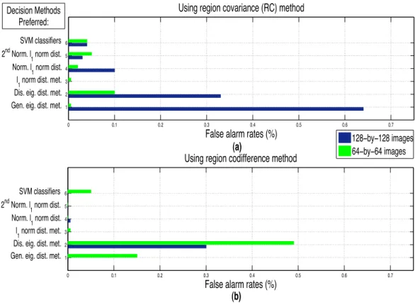
as input into SVM classifiers. However, for real-time applications, testing images using SVMs provides the lowest computational complexity.
Finally, the studies show that in most cases region codifference features are describing the ROIs that they represent better than the RC features. Thus, the target detection and false alarm performances are generally better when codifference matrices are used. The reader should recall that another advantage of using codifference matrices is the lower computational cost that they bring to the overall image classification system, as described in Section 2.3.
97.5 98 98.5 99 99.5 100 100.5 1 2 3 4 5 6
Target detection accuracies (%) Using region covariance (RC) method
97.5 98 98.5 99 99.5 100 100.5 1 2 3 4 5 6
Target detection accuracies (%) Using region codifference method
128ïbyï128 images 64ïbyï64 images (b) (a) Decision Methods Preferred: SVM classifiers 2nd Norm. l 1 norm dist.
Dis. eig. dist. met. Gen. eig. dist. met.
l
1 norm dist. met.
Norm. l
1 norm dist.
SVM classifiers
Gen. eig. dist. met. Dis. eig. dist. met.
l
1 norm dist. met.
Norm. l
1 norm dist.
2nd Norm. l
1 norm dist.
Figure 2.9: The target detection accuracies (%) obtained with various decision techniques using (a) RC and (b) codifference methods proposed.
0 0.1 0.2 0.3 0.4 0.5 0.6 0.7 1 2 3 4 5 6
False alarm rates (%) Using region covariance (RC) method
0 0.1 0.2 0.3 0.4 0.5 0.6 0.7 1 2 3 4 5 6
False alarm rates (%) Using region codifference method
128ïbyï128 images 64ïbyï64 images
2nd Norm. l1 norm dist. Norm. l1 norm dist. l1 norm dist. met. Dis. eig. dist. met.
2nd Norm. l1 norm dist. Norm. l1 norm dist. l1 norm dist. met. Dis. eig. dist. met. Gen. eig. dist. met.
Decision Methods Preferred:
SVM classifiers
Gen. eig. dist. met.
SVM classifiers
(a)
(b)
Figure 2.10: The false alarm rates (%) obtained with various decision techniques using (a) RC and (b) codifference methods proposed.
The results upto this point are obtained with 132 target and clutter training images. In Table 2.8, one can see the target detection accuracies and false alarm rates acquired using RC and codifference methods with l1 norm distance metric
and SVM classifiers after increasing or decreasing the number of target and clutter training images. As the number of training images increases, the target detection accuracies also increase. However, the behaviour of false alarm rates are unpredictable.
Table 2.8: The target detection accuracies and false alarm rates obtained with various numbers of training images
Number of training images
Target 76 132 174 220
Clutter 76 132 174 220
Simulation results Using RC method With l1 norm distance metric
Target det. 2664 2683 (99.29%) 2626 2627 (99.96%) 2585 2585 (100%) 2539 2539 (100%) accuracies False alarm 0 13346 (0%) 133461 (∼0%) 133460 (0%) 133460 (0%) rates With SVM classifiers Target det. 2663 2683 (99.25%) 2617 2627 (99.62%) 2585 2585 (100%) 2539 2539 (100%) accuracies False alarm 0 13346 (0%) 6 13346 (0.05%) 0 13346 (0%) 0 13346 (0%) rates
Using reg. codifference method With l1 norm distance metric
Target det. 2675 2683 (99.70%) 2626 2627 (99.96%) 2585 2585 (100%) 2539 2539 (100%) accuracies False alarm 0 13346 (0%) 1 13346 (∼0%) 0 13346 (0%) 3 13346 (0.02%) rates With SVM classifiers Target det. 2672 2683 (99.59%) 2626 2627 (99.96%) 2585 2585 (100%) 2539 2539 (100%) accuracies False alarm 0 13346 (0%) 1 13346 (∼0%) 1 13346 (∼0%) 2 13346 (0.01%) rates
Using k-Nearest Neighbor (k-NN) Algorithm
K-Nearest Neighbor (k−NN) algorithm is a method for classifying objects based on the closest training samples in the searched feature space. The classification of an object is decided according to the majority vote of its k neighbors in the training dataset. The neighbors stated here are the other objects that have smallest distances with the object to be classified.
The k− NN algorithm is used with the l1 norm distance metric on RC and
codifference methods. The majority of k training images providing smallest l1
norm distance with the test image assigns whether a test image belongs to a target or clutter. The target detection accuracies and false alarm rates achieved with increasing k values are presented in percentages in the following Figures 2.11 and 2.12. 10 20 30 40 50 60 70 80 90 100 97.5 98 98.5 99 99.5 100 k values
Target detection accuracies (%)
Using RC method on 128ïbyï128 images Using codifference method on 128ïbyï128 images Using RC method on 64ïbyï64 images
Using codifference method on 64ïbyï64 images
Figure 2.11: The target detection accuracies (%) obtained for increasing k values using l1 norm distance metric.
10 20 30 40 50 60 70 80 90 100 0 2 4 6 8 10 12 14 k values
False alarm rates (%)
Using RC method on 128ïbyï128 images Using codifference method on 128ïbyï128 images Using RC method on 64ïbyï64 images
Using codifference method on 64ïbyï64 images
Figure 2.12: The false alarm rates (%) obtained for increasing k values using l1
In Fig. 2.11, it is observed that using RC method leads to lower target de-tection accuracies with increasing k values. When region codifference method is considered, the target detection accuracies drop until k = 20, but rise again until the largest k value.
The false alarm rates increase gradually for both the RC and codifference methods, when k is increased. However, the rise is huge when RC matrices are used to represent the input images.
The responses of the methods presented here to the k− NN algorithm are similar for both 64-by-64 and 128-by-128 sized input SAR images. Commonly, the SAR image classification performance degrades for larger k values. There-fore, the k− NN algorithm brings extra unnecessary computational cost to the system as it does not provide any improvements for the methods presented in this chapter.
2.6.2
Using Principal Component Analysis (PCA) Method
The commonly used Principal Component Analysis (PCA) is applied to the MSTAR database, in order to make comparisons with the presented methods. PCA is basically an eigenvector-based multivariate analysis method which in-volves extracting a smaller number of uncorrelated variables named principal components from a number of possibly correlated variables [20]. This method is widely applied in many types of analysis such as neuroscience, face recognition, image compression due to its simple, non-parametric nature and ability to reduce data of high dimensionality to lower dimensionality.
The implementation of PCA includes the following phases: First a dataset is formed from the training images of the database represented by a M by N matrix, where M is the number of samples and N is the vector length, i.e. data dimension of each sample. The mean is subtracted from each data dimension.
The covariance of this new M by N matrix is calculated. Next the eigenvectors and eigenvalues of the covariance matrix are computed. Finally the determined number of principal components is selected to form a feature vector. The number of the principal components, which also corresponds to the length of the feature vector, is important and can be adjusted based on the dataset and performance results. Increasing the number of principal components may degrade the perfor-mance. In this work, using more than 8 principal components slightly reduces the target detection and classification performance. The best performance is achieved with 8 principal components. The same polynomial SVM kernel as in Section 2.6.1 is used to train and test these principal components. The numbers of target and clutter images in training and test datasets are given in Table 2.9. The target detection algorithm results using the PCA method are depicted in Table 2.10.
Table 2.9: Number of images used in training and testing studies for the PCA method
Number of train images Number of test images
Target 108 2651
Clutter 569 13445
Table 2.10: Target detection accuracies and false alarm rates achieved using PCA method
Input images Rates
(ROIs)
Target detection False alarm accuracies
128-by-128 2644/2651 (99.74%) 0/13445 (0%) 64-by-64 2647/2651 (99.85%) 0/13445 (0%)
The same database used for the PCA method is used on RC and codifference methods presented in this chapter. The decisions are made with l1 norm
dis-tance metric, which is one of the decision methods that gives highest detection performances. Furthermore, this metric provides the lowest computational cost
for the algorithm among other distance measures, as described in Section 2.6.1. The target detection and false alarm rates obtained are presented in Table 2.11. Table 2.11: Target detection accuracies and false alarm rates achieved using the distance metric defined in Eq. 2.9
Input images Rates (ROIs)
Target detection False alarm accuracies
Using RC 128-by-128 2634/2651 (99.36%) 0/13445 (0%) method 64-by-64 2642/2651 (99.66%) 0/13445 (0%) Using region 128-by-128 2649/2651 (99.92%) 0/13445 (0%) codifference method 64-by-64 2648/2651 (99.89%) 0/13445 (0%)
The RC and codifference features are also trained using a SVM classifier on the database used in this section. The prediction results made by the SVM classifier are presented in Table 2.12.
Table 2.12: Target detection accuracies and false alarm rates achieved using SVM as a classifier
Input images Rates (ROIs)
Target detection False alarm accuracies
Using RC 128-by-128 2638/2651 (99.51%) 0/13445 (0%) method 64-by-64 2647/2651 (99.85%) 0/13445 (0%) Using region 128-by-128 2649/2651 (99.92%) 0/13445 (0%) codifference method 64-by-64 2648/2651 (99.89%) 0/13445 (0%)
The results in Tables 2.10, 2.11 and 2.12 show that when region codifference matrix features are used with the two decision methods for both 128-by-128 and 64-by-64 sized ROIs, better target detection accuracies are achieved than the PCA method. This is as an expected result as the region codifference method is proven to be generally providing better detection performances than the RC method in the previous sections.
Moreover, it is observed that the false alarm rates acquired from the simula-tions are always 0%. This is mainly because higher number of clutter training
images is used in the decision process when compared to number of target train-ing images for the simulations implemented in this section.
2.7
Summary
In this chapter, a descriptive feature parameter extraction method from SAR images is proposed. The new approaches are based on RC and region codif-ference methods. Simulation results of target detection in MSTAR database are presented. The RC method delivers high detection accuracies and low false alarm rates. However, it is observed that the codifference method provides better performance than the RC method and PCA method with accurate SAR image classification performances. Furthermore, simulation results indicate that the best detection and false alarm rates are achieved when the l1 norm distance
metric is used to match two codifference matrix feature vectors instead of mea-sures involving computation of eigenvalues or using SVM classifiers. The work presented in this chapter is published in [22].
Chapter 3
Use of Directional Filters (DFs)
on Target Detection Methods
3.1
Introduction
Target detection in SAR images using region covariance (RC) and codifference methods is shown to be accurate in Chapter 2 despite the high computational cost. The proposed method in this chapter uses directional filters in order to decrease the search space. As a result the computational cost of the RC and codifference based algorithm significantly falls as the number of comparisons de-crease. Images in MSTAR SAR database are first classified into several categories using directional filters (DFs). Target and clutter image features are extracted using RC and codifference methods in each category. Features of the test dataset are compared to a lower number of features in the training dataset using l1 norm
distance metric in Eq. 2.9. Support Vector Machines (SVMs) which are trained using RC and codifference matrix feature vectors are also used in decision making within each category. Simulation results are presented.
In this chapter, a pre-processing stage based on directional filtering is in-troduced for SAR image classification using the RC and codifference algorithm proposed in the previous chapter. Directional filters were successfully used as a first stage in many applications including vector quantization and image cod-ing [23]-[27]. Regions of interests (ROIs) in SAR images are filtered uscod-ing two-dimensional directional-wavelet type filters in order to divide both target and clutter images into categories according to their orientations. Then the images are distributed into training and test datasets.
The output of the pre-processing stage is fed to the detection stage in which representative feature parameters are extracted using the covariance and codiffer-ence matrices of the ROIs. The distance between matrices is calculated using the l1 norm distance. The matrices are also used as SVM feature space parameters
for discrimination between target and clutter images. Simulations are carried out using a MATLAB computing environment (version R2009b). It is observed that the directional approach, when used with l1 norm distance, reduces the
computational complexity without decreasing the target detection accuracy in a significant manner in the MSTAR database. Target detection and false alarm rates are comparable to the methods in Chapter 2 which have higher computa-tional costs. The entire process is illustrated in Fig. 3.1.
Figure 3.1: Block diagram of the two-stage target detection process investigated in this chapter
The remaining part of this chapter is organised as follows. In Section 3.2, directional filters (DFs) which are used in the pre-processing stage of the algo-rithm are introduced. The target detection strategy of the two-stage system is described in Section 3.3. Simulation results are presented in Section 3.4 with comparisons of the proposed methods here to the existing methods.
3.2
Pre-processing Stage and Directional Filter
(DF) Design
The number of comparisons made in matching with target and clutter images causes a considerable rise in computational cost. The computational cost is mainly due to the straightforward distance computations with high number of training samples. This cost has to be reduced when one wants to scan large image regions at different locations. In addition, the target detection algorithm is also expected to be used in real-time applications. In this section, a pre-processing stage is proposed which consists of applying directional filters (DFs) to classify target and clutter images to categories according to their orientations. As the nature of this process suggests, smaller number of images are used within categories in decision of target or clutter images, and therefore computational cost of the target detection algorithm decreases significantly with the proposed pre-processing stage.
The design principle of the DFs used in this work is illustrated in Fig. 3.2. On the left hand side, 7-by-7 horizontal DF is shown. This filter is used as the template filter to design the other DFs. Along the horizontal axis, the filter coefficient values change from -1 to 1 in 7 steps in a linear manner. The other directional filters are produced from the template filter coefficient matrix by ro-tation. To obtain the first filter DF1 from the template DF, the outermost pixels are rotated clockwise by one unit as shown in Fig. 3.2. The second filter DF2 is
obtained from DF1 in a similar manner. In DF2, the inner filter coefficients are also rotated clockwise by one step. The DF3 is obtained from the DF2, and it is a diagonal filter. The DF4 and the DF5 are 90◦ rotated versions of DF1 and
DF2, respectively. Filters DF6-DF10 are symmetric with respect to DF1-DF5 on vertical axis, respectively. All the DFs are shown in Fig. 3.2. Samples of obtained target images can also be seen in Fig. 3.5.
Figure 3.2: Design of the directional filters (DFs)
As it can also be observed from the sample target and clutter images in Figures 2.5 and 2.8, the objects in SAR images are brighter to the top of them, providing natural vertical edges for all the ROIs. This property of the SAR images provides the images to be accurately classified into categories, as DF1-DF10 are designed to pick up the images having vertical edges between−90◦ and
90◦ rotation in 10 steps. However, a sharp vertical filter is avoided, because it
tends to bring up more images to its category than the other filters. Similarly, a sharp horizontal filter (see template filter in Fig. 3.2) tends to bring less number of images to its category compared to DF1-DF10.
In Fig. 3.3, the block diagram of the pre-processing stage is presented. First, the original 128-by-128 input target images obtained from the MSTAR database are cropped such that the targets and their shades are covered in the new 64-by-64 images, as described in Section 2.5. These 64-by-64-by-64-by-64 images are chosen simply because processing them is less costly and the studies in Chapter 2 show that they
give close detection performances to the 128-by-128 images. Then, these cropped images are decimated by a factor of two in each dimension before applying the directional filters in order to match the DF size with the targets. To prevent aliasing a simple 3-by-3 low-pass Gaussian filter is used during decimation. The coefficients of this filter, HLP F is as follows,
HLP F = 1 16 1 8 1 16 1 8 1 4 1 8 1 16 1 8 1 16
After applying DFs, the l1 norm of the output images are calculated as
MR = ||R(x, y)||1, where MR represents the magnitude of the image region R.
Finally, the cropped images are categorized under the number of the filter that they give the highest norm. As a result, the nth category contains the 64-by-64
target images that produces the highest l1 energy output to DF n. Same
oper-ations are also applied to 128-by-128 clutter images obtained from the MSTAR database. The cropped 64-by-64 target and clutter images form the ROIs (re-gions of interests), which are same as the 64-by-64 images used in Chapter 2.
Figure 3.3: Block diagram of the pre-processing stage
Finally, it should be noted that, besides decreasing the computational cost, dividing the SAR images into categories covers up a deficiency in the character-istics of the covariance and codifference matrices. In Sections 2.2 and 2.3, it is
clearly observed that RC and codifference matrix features are not rotationally invariant because the feature vector z that they are built up on also consists of values computed from the first and second derivatives in x (horizontal) and y (vertical) directions. The outputs of directional filters DF1-DF10 provide the objects in the SAR images to be rotationally similar. Therefore a rotational invariance is achieved by applying the pre-processing stage prior to the former target detection algorithm.
3.3
Target Detection Strategy
After distributing the images into categories, training and test datasets are formed from the images. Then, in each category, for each ROIs of the clut-ter and target images, RC and codifference matrices are extracted as explained in Sections 2.2 and 2.3. 25 bounded coefficients are Fig. 2.7 are sufficient features for target/clutter detection process. Two methods are considered in the decision of whether an image belongs to a target or clutter.
The first method involves distance computation through l1 norm. The l1
norms of the differences between the two covariance or codifference matrices’ feature vectors are used in decision of whether a test image is a target or clutter image. The l1 norm distance metric ρ is re-defined in the following equation.
ρ(C1, C2) = p % i=1 $ p % j=1 (|C1(i, j)− C2(i, j)|) & (3.1) where, C1, C2 is the covariance or codifference matrix of ROIs R1 and R2 belong
to a test and training image in a category and p is the number of items in the feature vector z in Eq. 2.1. There are two reasons why this metric is chosen for target detection simulations presented in this chapter: (i) This metric provides the simplest decision metric among other metrics used in Chapter 2 by calculating only the magnitude of the difference of features. (ii) The metric provides good target detection performance as summarized in Tables 2.4 and 2.11.
For making comparisons with the l1 norm distance based method, the matrix
coefficients from training images are used as feature parameters for training SVM classifiers. This method is also proven earlier to be accurate on target detection with results in Tables 2.7 and 2.12. Besides, SVM classifiers provide the least computational solutions in real-time applications for the SAR image classification problem. The matrix coefficients of test images are compared to the model generated in training phase. The final predictions are obtained according to the classification results of the SVMs which determine whether the input test image is a target image or a clutter image.
The block diagrams of the target detection stage in each category for the considered two methods are shown in Fig. 3.4.
Figure 3.4: Block diagram of the target detection stage applied in each category using (a) l1 norm distance metric in Eq. 3.1 (b) SVM classifiers.
3.4
Simulation Results
As explained in Sections 3.2 and 3.3, the methods presented here have two stages. Therefore in this section, the proposed algorithm is simply referred as ”two-stage”
method. The effect of each stage on the overall target detection performance is illustrated in this section.
As indicated before in Fig. 3.1, the first stage of the algorithm is pre-processing, where target and clutter images belonging to each category are deter-mined using directional filter (DF) outputs. Sample target images belonging to each category are shown in Fig. 3.5. Symbols of DFs are given above the filters. These symbols are used to simplify the tables presented in this section, as they show the orientation of the DFs. As Fig. 3.5 illustrates, the symbols show also the orientation of the targets, which are decided according to the DFs’ output that they represent.
The same training and test images as in Section 2.6.1 are used with the methods described in this chapter. The total numbers of target and clutter images divided into training and test datasets are given in Table 2.1. In the first simulation, training and test images are distributed into 10 categories, as mentioned in Section 3.2. Therefore, the number of target and clutter images in the training dataset, decreased to 10-15 in each category from 132 in the older studies (see Table 3.1). Eventually, the number of comparisons made between test and training images with l1 norm distance metric in Eq. 3.1 are reduced
by approximately 90%. This is the main reason for computational efficiency in using the two-stage approach. When the training dataset is put into SVM and models are created for each category, this computational efficiency is no longer available as the total number of images to be trained remains the same with the studies in Chapter 2.
Exact number of target and clutter training and test images at the output of DFs 1-10 is given in Table 3.1. Same numbers of target and clutter images are used in each category. The decisions are made by both using l1 norm distance
metric and SVM classifiers on RC and codifference features. Simulation results are summarized in Fig. 3.6, which includes target detection acccuracies and false alarm (incorrectly classified clutter images) rates for each category.
Table 3.1: Number of training and test images used for the two-stage methods working on 10 categories
Categories
1 2 3 4 5 6 7 8 9 10 Total
Number of training images
Target 12 15 14 11 14 12 15 11 13 15 132
Clutter 12 15 14 11 14 12 15 11 13 15 132
Number of test images
Target 140 338 304 213 321 142 358 275 194 342 2627
![Figure 1.1: Synthetic aperture radar (SAR) working principle (adopted from [3]).](https://thumb-eu.123doks.com/thumbv2/9libnet/5877116.121209/18.892.224.738.434.811/figure-synthetic-aperture-radar-sar-working-principle-adopted.webp)
![Figure 2.4: Targets in the MSTAR: (a) BMP-2 Armored Personal Carrier, (b) BTR-70 Armored Personal Carrier, (c) T-72 Main Battle Tank [5].](https://thumb-eu.123doks.com/thumbv2/9libnet/5877116.121209/30.892.225.737.460.840/figure-targets-armored-personal-carrier-armored-personal-carrier.webp)