Joint test for structural model specification

JOINT TEST FOR STRUCTURAL MODEL SPECIFICATION A Master’s Thesis by SERKAN YÜKSEL Department of Economics Bilkent University Ankara September 2006

JOINT TEST FOR STRUCTURAL MODEL SPECIFICATION

The Institute of Economics and Social Sciences of

Bilkent University

by

SERKAN YÜKSEL

In Partial Fulfillment of The Requirements For The Degree of

MASTER OF ARTS in

THE DEPARTMENT OF ECONOMICS BILKENT UNIVERSITY

ANKARA

I certify that I have read this thesis and have found that it is fully adequate, in scope and in quality, as a thesis for the degree of Master of Arts in Economics

--- Assist. Prof. Taner Yiğit Supervisor

I certify that I have read this thesis and have found that it is fully adequate, in scope and in quality, as a thesis for the degree of Master of Arts in Economics

--- Prof. Ülkü Gürler

Examining Committee Member

I certify that I have read this thesis and have found that it is fully adequate, in scope and in quality, as a thesis for the degree of Master of Arts in Economics

---

Assist. Prof. Ashoke Kumar Sinha Examining Committee Member

Approval of the Institute of Economics and Social Sciences

--- Prof. Erdal Erel Director

ABSTRACT

JOINT TEST FOR STRUCTURAL MODEL SPECIFICATION Yüksel, Serkan

M.A., Department of Economics Supervisor: Assistant Professor Taner Yiğit

September 2006

Aim of this thesis is to propose a test statistic that can test for true structural model in time series. Main concern of the thesis is to suggest a test statistic, which has joint null of unit root and no structural break (difference stationary model). When joint null hypothesis is rejected, source of deviation from the null model may be structural break or (and) stationarity. Sources of the deviation correspond to different structural models: Pure stationary model, trend-break stationary model and trend-trend-break with unit root model. The thesis suggests a test statistic that can discriminate null model from alternative models and more importantly, one alternative model from another. The test statistic that is proposed in the thesis is able to detect specific source of deviation from the null model. By doing so, we can determine the true structure model in time series. The thesis

compares power properties of the test statistic that is proposed with the most favorable test in the literature. Simulation results indicate the power dominance over the test statistics in the literature. Moreover, we are able to specify true alternative model.

Key Words: Unit root, Structural Break, Joint Hypothesis Testing, Monte Carlo Simulations

ÖZET

YAPISAL MODEL BELİRLENMESİ İÇİN BİRLEŞİK TEST Yüksel, Serkan

Master, İktisat Bölümü

Tez Yöneticisi: Yrd. Doç. Taner Yiğit

Eylül 2006

Bu tezin amacı, zaman serilerinde yapısal modelin belirlenmesini sağlayabilecek bir test istatistiği önermektir. Bu amaç doğultusunda, boş hipotez olarak birim kök ve yapısal kırılmanın olmadığı (ilk fark durağan modeli) model belirlenmiştir. Bu boş hipotezin reddedilmesi durumunda, boş hipotezden sapmaya neden olan alternatifler durağan yapı veya (ve) yapısal kırılmadır. Sapmaya neden olan yapılar ise: Durağan model, yapısal kırılmalı durağan model ve yapısal kırılmalı birim kök modelleridir. Bu tezde boş hipotez altındaki modeli alternatif hipotezlerden ayırabilecek ve daha da önemlisi alternatif modelleri birbirinden ayırabilecek bir test istatistiği geliştirilmiştir. Böylece, zaman serilerinde doğru modelin sınanmasını sağlacak bir test istatistiği oluşturulmuştur. Ayrıca, geliştirilen test istatistiği ile literatürdeki en başarılı test istatistiği Monte Karlo simülasyonlarıyla karşılaştırılmış ve bu tezde geliştirilen test istatistiğinin daha başarılı olduğu

gözlenmiştir. Bu durum, geliştirilen test istatistiğinin kullanımsal geçerliliğine işaret etmektedir.

Anahtar Sözcükler: Birim Kök, Yapısal Kırılma, Birleşik Hipotez Testi, Mote Karlo

ACKNOWLEDGEMENTS

I would like to express my gratitude to my thesis supervisor Assist Prof. Taner Yiğit for his guidance, patience and encouragements he gave me during the preparation of this thesis. His efforts brought my studies up to this point. I am truly indebted to him. I would like to thank to Prof. Ülkü Gürler and Assist. Prof. Ashoke Kumar Sinha for their insightful comments they made during my defense of the thesis.

My thanks also go to A. Banerjee and J. Y. Park for their quick help during the preparation of this thesis.

I especially would like to thank my teachers in Bilkent University and Bilgi University. They have introduced the excitement and the value of science to me.

Finally, I owe very special thanks to my mother, father and brother for their never lasting love and support from all the beginning of my life.

TABLE OF CONTENTS

ABSTRACT ... iii

ÖZET... v

ACKNOWLEDGMENTS... vii

TABLE OF CONTENTS ... viii

CHAPTER 1: INTRODUCTION ... 1

CHAPTER 2: LITERATURE SURVEY ... 8

2.1 Literature on Unit Root Hypothesis Testing ... 9

2.2 Structural Model Specification – Difference Stationary Models Versus Trend Stationary Models ... 13

2.3 Parameter Shift Literature... 23

2.4 Unit Root Hypothesis and Structural Break ... 26

2.5 Assessment of Literature and Open Questions ... 42

CHAPTER 3: TEST STATISTIC AND METHODOLOGY ... 45

3.1 Motivation ... 45

3.2 Model and Assumptions ... 47

3.3 Test Statistic ... 50

CHAPTER 4: MONTE CARLO SIMULATIONS ... 61

4.1 Simulations in General ... 63

4.2 Finite Sample Size Simulations ... 64

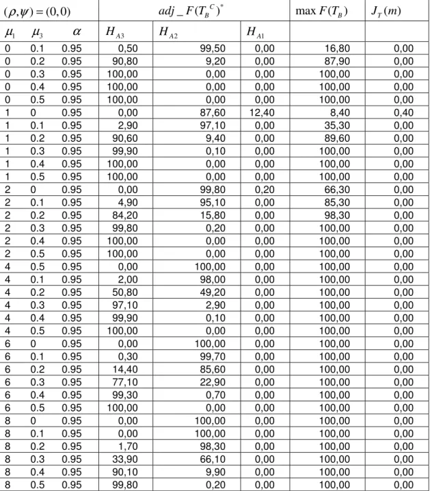
4.3 Finite Sample Power Simulations When H is True DGP ... 65 _A1 4.4 Finite Sample Power Simulations When H is True DGP ... 67 _A2 4.5 Finite Sample Power Simulations When H is True DGP ... 71 _A3 CHAPTER 5: SUMMARY AND CONCLUSIONS ... 73

CHAPTER 1

INTRODUCTION

Time series analysis has been dealt with the properties of the many macroeconomic and financial time series. Main concern of the researches in the time series is the question that: how macroeconomic and financial time series move over time? A major ongoing debate started after Nelson and Plosser (1982) try to characterize the dynamic properties of macroeconomic and financial time series. Nelson and Plosser (1982) have claimed that, shocks hitting the economy have a permanent effect rather than temporary effect and the long run movement in the time series is altered by these permanent shocks. Using some statistical techniques that are proposed by Dickey and Fuller (1981), Nelson and Plosser (1982) have found that time series contains unit autoregressive root. Nelson and Plosser (1982) claim that time series follow a difference stationary model. Difference stationary model characterization of the macroeconomic variables indicates that, long run movement of the time series do not fluctuate around a

steady state long run value but rather the movement is totally altered by the shocks that are hitting the economy. Then implications of the difference stationary model interrogate the steady state assumptions in the economics. Since justification of the difference stationary model deters underlying principles of economics, the research that is proposed by Nelson and Plosser (1982) has stimulated much interest.

Some researchers have challenged the characterization of the time series as a difference stationary framework which is suggested by Nelson and Plosser (1982). In particular, Rappaport and Reichlin (1989) and Perron (1989) argue that, log output is stationary around broken time trend whereas the date of break is the years of Great Depression. In brief, Perron (1989) shows that, Nelson and Plosser have failed to account for trend break in the GNP and they have accounted this one time innovation shift as long lasting rather than it was in fact one time innovation. If years of the Great Depression are specified as the time that structural change has occurred, then the unit root hypothesis is rejected in favor of the trend-break alternative. Perron (1989) claims that, the reason for failure to reject the unit root hypothesis is a consequence of misspecification in the trend function, especially a one time structural break in trend function. Perron (1989) has proven that, when in fact the trend break model is the true structure of the time series, unspecified structural break raises spurious evidence for unit root hypothesis. If trend-break alternative is not specified in the test procedure, unit root hypothesis cannot be rejected. After Perron (1989) made a critic of Nelson and Plosser, literature has been developed with the attempts to understand the true nature of time series: difference stationary model versus trend break stationary models.

all, if the trend stationary model is correct, then some studies as Cochrane (1988) and Cogley (1990) have put too much importance to the innovations in GNP. Non rejection of the unit root hypothesis is counter evidence against business-cycle hypothesis. When structural break is not accounted, then false empirical inferences may arise from the spurious conclusion of the unit root behavior. Cointegration analysis is based on the presumption that the time series follow a unit root pattern. In fact, if time series follow trend-break stationary pattern rather than difference stationary, then empirical relevance of the literature in econometrics on unit root and cointegration is brought into question.

Trend-break alternative model that is presented by Perron (1989) has been criticized for two reasons. First, Perron (1989) determines break date by presumption that, date of break coincides with years of Great Depression. Break date is specified prior to any knowledge up on data. The assumption that break date is known a priori was criticized by many authors. Christiano (1992) shows that the pretest examination of data can make important difference on Perron’s conclusion. Christiano (1992) stated that, break date selection affects critical values of the test statistic which makes non rejection of the trend break stationary model dependent on the selection of the break date. Christiano states that, reliable test should consider break date as unknown a priori. The method that is suggested by Christiano (1992) relies on the standard sampling theory. The date of break is chosen independent of prior information about data. Also Banerjee, Lumsdaine, Stock (1992), Zivot and Andrews (1992) Perron and Vogelsang (1992) argue that the choice of break should be treated as unknown. Extensions of the trend break alternative model have been proposed by many authors. Specifically, Zivot and

Andrews (1992), Banerjee, Lumsdaine, Stock (1992), Perron and Vogelsang (1992), Perron (1997), Vogelsang and Perron (1998) adopted Perron’s (1989) methodology for each possible break-date in the sample, which yields a sequence of the statistics that is in interest. Some algorithm that maximizes evidence against null hypothesis can be constructed from the sequence of the statistics, to determine break date.

Second criticism is based on the selection of the alternative form of trend break model. If the date of break is treated to be unknown, then the form of the break is also unknown. Then the determination of the form of break in alternative hypothesis becomes important. Sen (2003) notes that, if the alternative form of structural break does not coincide with the true form of break that time series follow, then test statistic will fail to reject difference stationary model because of wrong specification of the alternative hypothesis. Test for difference stationary model versus trend break stationary model should take into account all possible form of breaks in order to avoid specification errors that Perron has highlighted. Sen (2003) suggests that alternative form of break should be most general in order to avoid misspecifications. Alternative break forms that Perron has considered are: break in the mean of trend function (Crash Model), break in the slope of trend function (Changing Growth Model) and break in both mean and slope of trend function (Mixed Model). Sen (2003) has proposed a joint null hypothesis of unit root and no break in both mean and slope of trend function. Sen (2003) used the maximal F statistics that is proposed by Murray (1998) and Murray and Zivot (1998). Test is sequentially computed over range of possible break dates so maximum F test is also independent of break date specification. Then, joint null

hypothesis corresponds to the difference stationary model. Non rejection of the null hypothesis indicates the appropriateness of the difference stationary model for time series. Joint null hypothesis incorporates with possible trend breaks of both types. Non rejection is not sourced by the unaccounted trend breaks because the null hypothesis includes restriction of no structural break with any possible form. Joint null hypothesis is not only unit root test but also test for no structural break pattern in the time series.

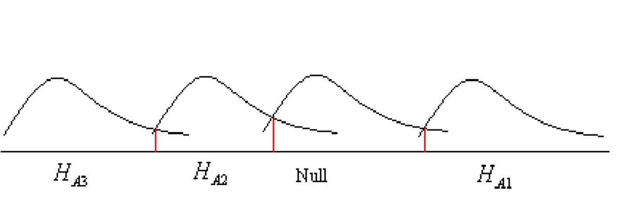
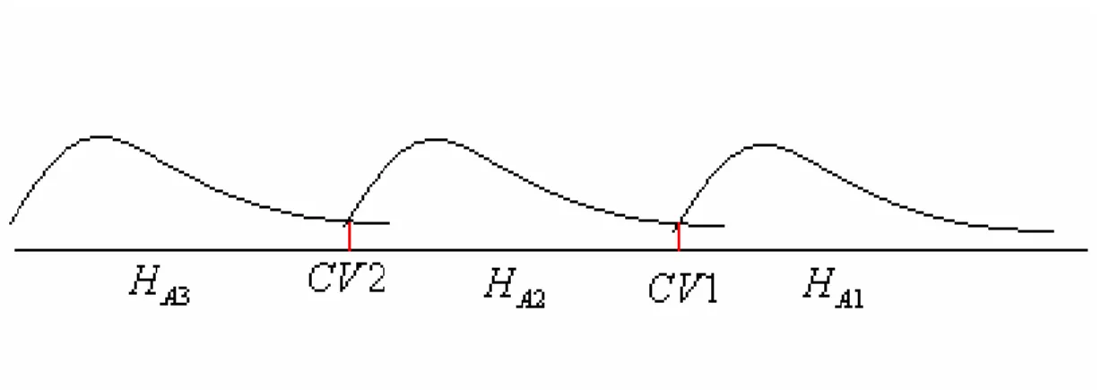
However, when joint null hypothesis is rejected, alternative hypothesis is too general to specify a structural form for time series. In other words, rejection of the test statistics does not provide us enough inference on the alternative hypothesis to conclude specific structural form. Since the null hypothesis is the joint mixture of unit root and no structural break, null hypothesis is too restrictive, when test is rejected, alternative may involve three model specifications according to source of deviation from the null model. According to source of deviation from the null model, there exist three alternative models: 1) Pure stationary model: Stationary and no break alternative. 2) Trend break stationary model: Stationary with some form of break. 3) Trend break model with unit root pattern: unit root behavior with structural break.

In our study, we aim to propose a test statistic that can exactly determine the specific structural model that time series pertain. We suggest a test statistic that can discriminate null model from these three alternatives. Moreover, our test statistic is able to discriminate one alternative from another. Additional to the difference stationary and trend break stationary models, we specify pure stationary model and trend break with unit root pattern model. Additional models are

alternatives to the difference stationary null model. Additional alternative models are not covered in the literature. According to source of deviation from alternative, we specify two additional alternative models. When time series follow additional structure models, existence of their structure increases evidence against difference stationary model; they can be specified as alternatives to the difference stationary model. Secondly, we aim to propose a test statistic which has joint null of unit root and no structural break where break date is not determined a priori and break date is not affected by the unit root property of the time series.

Our test is motivated from the methodology that is suggested by Andrews (1992) and Andrews and Ploberger (1994). We use combination of the F maximum and the J test that has been proposed by Park (1989) and Park and Choi (1991). From the methodology of Vogelsang (1998), we utilize the property that J statistic converges to zero for stationary behavior of the time series and J statistic converges to a constant for unit root pattern. We adjust F max statistics with J value in order to determine one specific alternative hypothesis when joint null is rejected. By doing so, we can suggest a test statistic that can differentiate three different alternative structural models. Using joint null hypothesis of unit root and no structural break allow us to present a test statistics that can both test for unit root and structural break. We use similar methodology to Vogelsang (1998, 2003). But, rather than using only joint null of no break of both types; we propose joint null of unit root and no structural break. We are able to specify difference stationary model in the null hypothesis. The test statistic that we propose does not only test for unit root and (or) structural break, null and alternative hypotheses correspond to different structural models of time series. Moreover inclusion of unit

root pattern in to the test statistic reduces the possible source of size and power distortions. Appendix section shows that our test statistic has better power properties than the test statistics in the literature.

Rest of the study is organized as follows. Chapter 2 consists of the literature survey and various comments on unit root hypothesis and structural break. Various model specifications and various test statistics that are presented in the literature are included in this section. Chapter 2 consists of various attempts to specify unit root or (and) structural break forms. Chapter ends up with the assessment of the literature and the shortcomings of the tests in the literature. Reason for inability to specify a structural model for time series has been discussed. Chapter 3 gives a detailed methodology of the test statistic that is presented in this study. Chapter 4 includes power and size Monte Carlo Simulations with comparison to the previous most powerful test. Chapter 5 concludes and includes the arguments for further research.

CHAPTER 2

LITERATURE SURVEY

In this section, the literature survey of the research is presented. First the literature on unit root hypothesis is discussed. Joint hypothesis test includes testing for unit root. Preliminary discussion of unit root hypothesis will clarify the developments in the joint test. Literature on unit root hypothesis has extended with testing for unit root with a linear time trend in the model. Secondly, trend break literature is included into agenda. Evolution of the trend break test into the joint hypothesis test holds particular importance for model specification of the time series. Literature of this evolutionary process has been presented in this research. Other part of the joint test is the test for structural break. Structural break literature is also summarized in this research. Literature has been discussed by the virtue of extensions to the hypothesis testing on the question of the true behavior of time series. This discussion has been concluded by the open questions that we aim to answer in this research.

2.1 LITERATURE ON UNIT ROOT HYPOTHESIS TESTING

Unit root hypothesis is particularly important in terms of the well established properties of the long-run equilibrium in economics. Therefore testing for unit root hypothesis has been one of the important areas of macro-econometrics. Unit root representation of the time series has been firstly presented by Dickey and Fuller (1979). In their seminal article, brief introduction to unit root autoregressive time series has been presented.

To follow their article, let T observations Y₁,K,Y_{T be generated by the} model Y_t =αY_t−1+ε_t, where ε_t is a sequence of independent normal random variables with zero mean and variance 2

ε

σ and t is time script. Properties of the regression estimator of α are obtained under the assumption that α ≤ . Because 1 when α >1, time series is not stationary and the variance of the time series grows exponentially as t increases. Hence asymptotic distribution derivation may not be feasible. The time series with α =1 is sometimes called as random walk. The null hypothesis of unit root (α =1) holds interest in economic applications. The class of models presented in Dickey and Fuller (1979) are:

1 t t t Y =αY₋ +ε (2.1a) 0 1 t t t Y =µ +αY₋ +ε (2.1b) 0 2 1 t t t Y =µ +µ t+αY₋ +ε (2.1c)

2 1/ 2 1 1 ˆ ˆ ( 1)(se c ) τ α − = − (2.2a) 2 1/ 2 2 2 ˆ ˆ_µ ( 1)(se c ) τ α − = − (2.2b) 2 1/ 2 3 3 ˆ ˆ_t ( 1)(se c ) τ ₌ α₋ − (2.2c) For k=1, 2, 3 2 k

se is the corresponding regression residual mean square from the models. Also c_k is lower-right element of u_k where u₁=(Y_t−1), u₂ =(1,Y_t−1),

3 (1, , t 1)

u = t Y₋ . Limit distributions and their representations are shown in the Dickey and Fuller (1979).

After Box and Jenkins (1970) and Box and Pierce (1962) used the test of autocorrelation function of the deviations from fitted model, unit root testing proposed by Dickey and Fuller (1970) has been the test of appropriateness of the time series model. Non-rejection of the unit root null hypothesis is taken as an evidence for unit root behavior of the time series. Unit root pattern implies that, time series possess difference stationary model. First difference of the time series follow a stationary pattern. Then, time series have steady state values so that analysis of time series is feasible.

Autoregressive time series with unit root has taken much interest after Dickey (1976), Evans and Savin (1981, 1984) made forefront research. Random

walk characterization such as ∆Y_t =ε_t where 2

~ (0, )

t iid

ε σ , is a strong

assumption. Hall (1978) showed the convenience and importance of the random walk hypothesis. Philips (1987) allows for more general weakly dependent and heterogeneous distribution theory for the random walk and allow for more general ARMA (1, 1) errors with single unit root. Philips (1987) notes that, the

representation in (2.1a) can be a stochastic process generated as Y_t =S_t+Y₀ in

terms of partial sums,

1 T t t t S ε =

=

∑

condition Y₀. Initial conditionY₀ can have specific distribution so that α ≥1

alternative has been covered. Limiting distribution of the standardized sums is presented in second chapter of Philips’s paper. From Dickey and Fuller (1970), OLS estimator of α in (2.1a) and t-statistic is:

1 2 2 1 1 1 1 1 ˆ ( 1) { ( )}/{ } T T t t t t T α T− y y y T− y − − − − =

∑

∑

∑

∑

Philips derives new unit root test by defining new transformation estimator Z_α for ˆ

( 1)

T α− and transformation regression test statistic Z_t instead of regression t-statistic such as:

2 2 2 2 1 1 ˆ ( 1) (1/ 2)( ) /( ) T T t Z_α T α s s T− y ε − = − − −

∑

∑

∑

s and s_ε2 are estimates of variance of errors (σ2_ε) and variance of α (σ2). These parameters should be estimated consistently. Philips showed that;

2 1 2 1 1 ( ) T t t s_ε =T−

∑

∑

∑ ∑

are consistent estimates of 2 ε

σ and 2

σ . Philips (1987) has proposed an alternative unit root test to Dickey and Fuller’s t-test. Theory of the research relies on the weak convergence. Characterization of the limiting distributions (2.3a) and (2.3b) are rather simple in terms of functionals of Brownian Motions.

Philip’s unit root test transformation is related to the model (2.1a) corresponding to the class of models defined by Dickey and Fuller. But the models with drift and trend have not been covered in Philips (1987). This gap in the literature of unit root has been filled by Philips and Perron (1988). Two more models that correspond to the class of Dickey and Fuller are introduced by Phillips and Perron (1988). The models are:

0 1 t t t Y =µ +αY₋ + ε (2.6) 0 2( (1/ 2) ) 1 t t t Y =µ +µ t− T +αY₋ + ε (2.7)

Then, regression t-statistics are:

2 ˆ 1 1 ˆ ˆ ( ){ ( ) }/ T t t t_α = α α−

∑

Here, ˆs and s% are the standard errors of regressions of (2.6) and (2.7) as before.

3

c is lower right element of ₃ (1, (1 ), ₁)

2 t

u = t− T Y₋ .

Philips and Perron (1989) cite the importance of the innovations in the limiting distributions. When innovations are non-orthogonal andσ ≠ σ2 _ε2, the Dickey and Fuller t test does not have the asymptotic size. Limiting distributions depend the nuisance parameters 2

σ and 2

ε

elimination of nuisance parameter is a result of having 2 T

s rather than ε = ∆ . _t y_t

Extended models (2.6) and (2.7) accommodate with a fitted drift and a time trend so that they may be used to discriminate between unit root (difference stationarity) and stationarity around a deterministic trend. These extended models have better power compared to the previous no drift and no trend model. When many time series are simulated to be stationary about deterministic trend, percentage of the simulations that are rejected increase with extended model specification. The conclusion that Philips and Perron (1987) have reached made an influence on research. Many researchers suspect that unit root test is affected by inclusion of trend function into the model. When trend function is not included into the model, misspecification of trend parameter increases the evidence for non-stationary behavior and unit root hypothesis is not rejected erroneously. From the Monte Carlo simulations of the Perron and Philips (1987), one can claim that, maintenance of the trend parameter may affect the results of unit root tests. Theoretical literate have been developed with modifications of the unit root tests with trend function specified alternatives whereas empirical application of unit root hypothesis has attracted more attention. There is good summary of the research on this topic by Campbell and Perron (1991).

2.2 STRUCTURAL MODEL SPECIFICATION – DIFFERENCE STATIONARY MODELS VERSUS TREND STATIONARY MODELS

model specification of the time series. After Nelson and Plosser’s stimulating paper, one of the areas of interest in economics has been the application of unit root testing. The view that most economic time series are characterized by unit root behavior has become prevalent. Until Perron (1989) highlighted the importance of the structural model specification, literature has been developed on the empirical area of the unit root testing. After Philips and Perron’s research, maintenance of trend functions in the models have not been considered seriously. However, Perron (1989) indicated that when true data generation has a one time change in trend function, unit root tests fail to reject the trend stationary model. Perron (1989) characterize unit root test with the trend break model alternative. Different characterizations of the trend break alternatives are presented in Perron’s research. Perron has not only considered trend extended model, but also specified alternative trend-break stationary models. Then testing for unit root is enlarged to structural model specification with trend-break alternative. When unit root hypothesis is rejected in favor of the trend-break alternative, there is evidence for trend-break stationary model. Therefore unit root test has played the role for determining difference stationary versus trend-break stationary model specification. According to Perron, standard Dickey and Fuller (1979) unit root test cannot reject the unit root hypothesis, when in fact true data generation mechanism is that of trend break stationary. Spurious conclusion of the unit root testing may lead to incorrect empirical inference. Perron (1989) showed that even asymptotically stationary fluctuations of trend break model cannot be rejected.

Perron extends the analysis of Philip’s to a more general case which allows for one time change in the trend function. When Philips has considered trend

extended model, null hypothesis was unit root and alternative hypothesis was trend stationary model. Perron has allowed a break in the trend function which has three alternative forms. Null hypothesis of unit root has been considered for different three forms:

Model (A) y_t =µ₀+dD T( _{B t}) +y_t−1+ ε _t (2.10a)

Model (B) y_t =µ₀+y_t−1+(µ₂−µ₀)DU_t+ ε _t (2.10b) Model (C) y_t =µ₀+y₋₁+dD T( _{B t}) +(µ₂−µ₀)DU_t + ε _t (2.10c) Here in these representations, D T( _{B t}) = if 1 t =T_B+ and 0 otherwise; 1 DU_t = if 1

B

t>T and 0 otherwise. A L( )ε =_t B L v( ) _t, v_t ~iid(0,σ2). A L( ) and B L( ) are

'

p th and q th' order polynomials in the lag operator L. Corresponding alternative hypotheses are:

Model (A) y_t =µ₀+βt+(µ₂−µ₀)DU_t+ ε _t (2.11a)

Model (B) y_t =µ₀+β₁t+(β₂−β₀)DT_t+ ε _t (2.11b)

Model (C) y_t =µ₀+β₁t+(µ₂−µ₀)DU_t+(β₂−β₁)DT_t + ε _t (2.11c) Here in these representations, DT = −t T_B if t>T_B and 0 otherwise. T_B is the break date. Perron (1989) has considered three alternative forms of breaks. First, it is crash model (Model (A)) which allows for one time change in the intercept of the trend. Second is changing growth model (Model (B)) which allows for one time change in slope of trend function. Third is mixed model (Model (C)) which allows a change in both intercept and slope of the trend function. Perron states, when structural break alternative included into specification of the time series, the unit root hypothesis can be rejected in favor of the trend-break alternative. Basic

Dickey Fuller unit root test gives false results due to omitted variable of trend function or misspecification of the trend with breaks. When breaks have not been taken into account, residuals increase so that unit root null cannot be rejected. However, if data is separated into sub-periods at the time of break, critical values of t-statistic decrease significantly so that unit root hypothesis is rejected.

Perron’s analysis is important because of the statement: unaccounted structural breaks lead to spurious results of non-rejection of the unit root test. Estimation of nuisance parameter is highly affected by the trend behavior. Moreover, Perron has presented alternative representation of the time series such as trend-break stationary model. Perron suggests specification of the unit root test from these models:

0 1 1 ( ) k A A A A t t B t t i t i t i y µ θ DU β t dD T α y₋ c y₋ = = + + + + +

∑

∑

∑

∆ is included to reduce the autoregressive effect on nuisance parameter. Lag length k is selected by information criteria. The null hypothesis of unit root imposes restrictions α =1, β =0, γ =0 for representations in (2.14a-c). For the alternative models, asymptotic distributions of the t-statistics t_αA, t_αB, t_αC have

been derived. (For i=A, B, C)

years, Perron uses same data set of Nelson and Plosser applying to his methodology. Perron finds evidence against unit root hypothesis. When alternative model is set up as a trend break model with specified break dates, unit root hypothesis is rejected.

Rappaport and Reichlin (1989) confirmed the Perron’s conclusion. Rappaport and Reichlin noted that when alternative model is specified as segmented trend model rather than just trend stationary model, test statistic support segmented trend model. Both conclusions of Perron and Rappaport and Reichlin indicate that, difference stationary model cannot be approved by unit root test without putting trend-break into the test procedure. Empirical findings of Nelson and Plosser, Stulz and Wasserfallen (1985), Campbell and Mankiw (1987, 1988), Cochrane (1988), Hall (1987), Gould and Nelson (1974), Blanchard and Summers (1986) are brought into question.

After Perron has proven the spurious nature of the unit root test when alternative model is not specified as trend-break model, various questions have arisen in the literature. First of all, in Perron’s analysis, choice of the break date depends on visual inspection of the data. Determining break date without any diagnostic tests has been attacked by many authors. Christiano (1992) argues that, the date of break should not be chosen independent of the test procedure. When break date is exogenous to the testing procedure, then critical values are higher according to true size. Hence, rejection of the null hypothesis in favor of the alternative may be also spurious.

0 1 0 k i t j t j t j y µ θdt βt αy₋ c y₋ = ∆ = + + + +

∑

In equation (2.13), Perron’s modified augmented Dickey and Fuller test which has null hypothesis of α =β =θ =γ =0. Perron suggests comparing the t-statistic on

, t_α

α with critical values tabulated in his article where break date has been determined without pre-test of the data. Christiano suggests a methodology which allows for the selection of the break date as a function of the data being tested. He extends Perron’s analysis testing the same null hypothesis with F statistics for

t T

∀ ∈ with corresponding null hypothesis. Maximum value of F test will indicate the break date from the sequence of F statistics for ∀ ∈t T.

Secondly, Christiano suggests that, the lag length parameter k should also be selected with a methodology. Level of the lag truncation parameter k should be parallel to the significance of the parameter c_k. From maximum possible value of

k, the latest insignificant value of k according to diagnostic tests should be excluded. Choosing appropriate level of k* depends on the information criteria. Reason to include additional k* extra parameters c_k* is to get rid of the possible

autocorrelation as explained before. According to Christiano, Perron’s conclusion is a consequence of choosing break date a priori. When lag length parameter and break date are selected by data dependent methods, Christiano found contradictory evidence to trend stationarity model in GNP.

Perron and Vogelsang (1992) suggest another unit root test that is robust to the date of break specification. They have tested unit root hypothesis in the presence of mean break with application to the purchasing power parity hypothesis. According to Perron and Vogelsang (1992), assuming that date of break is known a priori is inappropriate. Their trend break alternative is crash

model (Model A), corresponding to the Perron (1989). For one time change in the level at time T_Bsuch that 1<T_B <T. They have parameterized the null hypothesis of unit root such that: y_t =D T( _{B t}) +αy_t−1+ ε . _t D T( _{B t}) = if 1 t=T_B + and 0 1 otherwise. Assumption on ε is consistent with the previous literature. Under the _t mean break alternative:

0 ( )

t B t t

y =µ +D T + ε (2.14)

They use t statistic for α =1 in the following regression, which nests the null and alternative hypotheses: 1 1 0 ( ) k k t i t i t t i t y =

∑

∑

They have suggested another method to choose date of break. T_B is chosen such that t i T k_α( , _B, ) is minimized for i=A, B, C models and k∈[0, max]k . kmaxis the upper bound of lag length. The selection of k was made with objective of getting the autocorrelation variance properties of the fitted residuals to resemble the assumptions made in the bootstrap simulations in the paper. As a result, k =4 is the lag length that is chosen by Perron and Vogelsang (1992). When break occurs at time T_B, it increases the absolute value of t-statistics for null of α =1. Hence, the mean break date is determined when evidence against the null hypothesis is maximized. So for t-test T_Bis determined from algorithm: inf _{(1, )} ( , , )

B

T∈ T t i T kα B .

The method that is presented by Vogelsang and Perron is similar to the previous methods in which the date of break is specified according to date when evidence against null hypothesis is maximized. They apply their methodology to test for purchasing power parity hypothesis to find evidence for trend stationary

model when mean break is utilized.

Another paper on this topic is proposed by Zivot and Andrews (1992). In their research they have cited the method proposed by Christiano (1992). Zivot and Andrews (1992) made critics of Christiano because of determining break dates solely by bootstrap methods. Zivot and Andrews (1992) used t-min statistic to determine date of break. Similar to Christiano (1992), Zivot and Andrews (1992) concluded that Perron’s unit root tests are biased towards rejecting the unit root. But the break dates found by Zivot and Andrews are different from the break dates found by Perron. Unit root hypothesis is not rejected for some series of Nelson and Plosser (1982). Only nominal GNP, industrial production series are found to be trend stationary. However inability to reject the null hypothesis of unit root should not be taken as an evidence for accepting the null. Rejection indicates the inappropriateness of the null hypothesis against the alternative hypothesis. Specification of the alternative hypothesis is also important. Main reason for contradicting evidence in various papers is to specify different alternative forms of break. Perron and Vogelsang have considered crash model alternative whereas Christiano and Zivot and Andrews have specified mixed model alternative. Question of the break date specification should be incorporated with specification of the alternative form of break. In more general sense, when difference stationary versus trend-break stationary model is tested, alternative form of the trend-break plays important role.

More general attempt to determine unit root hypothesis and trend-break alternative has been given by Banerjee, Lumsdaine and Stock (1992). Different from previous literature, Banerjee, Lumsdaine and Stock (1992) tried to make unit

root test and structural break tests together with general form. When date of break is assumed to be unknown, then existence of the trend-break should be tested. They perform a test that incorporates both unit root hypothesis and trend-break hypothesis in the null hypothesis. By doing so, they are able to specify the possible form of trend-break in the null hypothesis. Rejection of the null does not only indicates inappropriateness of the unit root null but also inappropriateness of the no trend-break restriction.

In order to test for unit root and structural break, sequential test is suggested. Sequential test has advantage of testing unit root with trend where alternative is trend-break for specific type of break. They consider both Crash Model alternative and Changing Growth Model alternative. Another advantage of the test is to have a joint null hypothesis. Also more than one algorithm is presented to choose break date. As an extension, recursive and rolling tests are suggested for unit root testing. But those tests do not incorporate with structural break test. Model is:

0 1 1( ) 2 1 ( ) 1

t B t t L t

y =µ +µ τ T +µ t+αy₋ +β L ∆y_{− −} + ε (2.16)

1(TB)

τ captures the possibility of a trend-break. For Crash Model (Case (A)),

1(TB) 1(t TB)

τ = > . For Changing Growth Model (Case (B)),

1(TB) (t TB)(t TB)

τ = − > . Testing for µ₁= corresponds to structural break test for 0

both case A and B. However under the null hypothesis joint null is µ₁=0, α = . 1 A transformation regression Z_t for set of variables and transformed parameter vector θ are defined. The estimator of the test statistic computed over T

observations for k=k k₀, ₀ +1,...,T−k₀ where k₀ =λ₀T . λ₀ is the trimming value of initial fraction of T. The stochastic process constructed from the sequential estimators and Wald test statistic is:

1 1 1 1 1 1 ( ) ( ( ) ( ) ') ( ( ) ) T T t t t t Z T Z T Z T y θ λ λ λ − λ − − − =

∑

∑

∑

∑

F λ is computed for every λ∈(λ₀,1−λ₀). If any break of specified form exists, then it increases the F_T( )λ statistics. Maximum value of the F_T( )λ is the best candidate from the sequence of the F_T( )λ statistics. T_B =λT is the break date

such that ( ) max ( )

B

T T

F λ = F λ . Test statistic is denoted as F_TMAX( )λ . F_TMAX( )λ is a Wald type test which also tests for existence of break. Banerjee, Lumsdaine and Stock (1992) have used Wald type F_TMAX( )λ test by utilizing the nature of the Wald test which allows testing for more than one parameter. Unit root and specific break type are tested together. By doing so, date of break is also determined by data dependent methods. Also, Banerjee, Lumsdaine and Stock (1992) compare various tests that take place in the literature. They propose Monte Carlo simulations to compare power properties of these various statistics. Monte Carlo simulations of Banerjee, Lumsdaine and Stock (1992) indicated that, sequential Wald type test is more accurate to detect break dates. Moreover F_TMAX( )λ statistic has power superiority over other test statistics. Their simulation results confirms

Perron’s conclusion. Basic Dickey and Fuller t-test fails to reject unit root when in fact data generation process contains trend-break stationarity. According to Banerjee, Lumsdaine and Stock (1992), Christiano failed to reject unit root hypothesis because of using bootstrapped critical values. When they apply their methodology to the growth rates, they have concluded that some countries’ GNP follows unit root.

DeLong etc. all. (1992) tested for I(1) versus trend-break stationary model with joint test. They have inverted unit root hypothesis to the joint hypothesis with null hypothesis α =1, µ₂ = with consistent notation with Banerjee, Lumsdaine 0 and Stock (1992). DeLong etc.all. (1992) develop a similar test which has size adjusted power for nuisance parameter, they have analyzed the power results of the joint test concerning dependent variables α and(y₀−µ₀) /σ . They have reached the conclusion that unit root tests have low power against plausible trend stationary alternatives. Moreover, there are some cases unit root hypothesis is rejected in favor of the trend-break alternative and trend-break alternative is rejected in favor of the unit root alternative. This results does suggest that inferences of the test of integration is fragile and also using more restricted null of unit root with no breaks works better with this nature of fragility. Nature of the test affects results. When no break restriction is put in null hypothesis, form of the break that is specified in the null hypothesis is also important. But those papers have put limited effort to research on the null of unit root with general form of no structural break. DeLong etc. all. (1992) only concluded that it is premature to accept difference stationary model with basic unit root tests.

2.3 PARAMETER SHIFT LITERATURE

Banerjee, Lumsdaine and Stock (1992) shifted the unit root testing against trend-break alternative to more general joint test. When joint null is α =1, µ₂ = , 0 testing this null hypothesis is a kind of test for structural break. Trend break test is a distinct form of structural break. In order to understand model specification literature, it is of partial interest to understand structural break literature.

Before Banerjee, Lumsdaine and Stock (1992), structural break test is accounted for only change in parameters and it’s linkage to the macroeconomic time series was not that much appealing in empirical literature. Structural break literature begins with Chow (1960) test for breaks in the regression. Main concern of the Chow (1960) was to asses the test of equality between set of coefficients in two linear regressions. By residual based test, regime stability or regime change has been concerned. Let y₁ =X₁β₁+ ε and let m additional observations specified ₁ by the regression y₂ =X₂β₂ + ε . Test of equality between parameters has null ₂ hypothesis H₀:β₁=β₂ =β such that y=Xβ+ ε. Test depends:

1 2 2 ˆ1 2 2 2 1 2 2( 1' 1) 1' 1 d y X β X β X β X X X − X = − = − + ε − ε (2.19) 2 / var( )

d d will be distributed by F(1,n−p) for n observations and pregressors. This test is based on the prediction interval for one new observation. The sum of squares of the residuals under null hypothesis will be equal to the sum of squares of the residuals under alternative plus sum square deviations between two sets of

estimates of y. Idea of the Chow Test is to obtain sum of squares of residuals under the assumption of equality between parameters and the sum squares without assumption of equality. The ratio of the difference between these two sums to the latter sum, adjusted for the corresponding degrees of freedom will be distributed as the F(1,n−p) ratio under the null hypothesis. This test is the basic version of the Wald test. As a matter of fact, when null hypothesis is α =1, µ₂ = , 0 µ₂ = part 0 of the null hypothesis tests for equality of parameters before and after the possible break date.

Another structural break test is proposed by Quandt (1959). Idea is to test for break in time t* from T observations. Possible structural break date t* has been chosen to minimize λ_{= σ σ}(ˆ ˆ₁t T t₂−) /_σˆT

. σ and ˆ₁ σ are estimated variance from first ˆ₂ and second regressions which are given below and _σˆT

is the aggregated estimated variance. Model is presented in Quandt (1959) as:

1 1 i i i y =a +b x +u for i=1,...,t 2 2 i i i y =a +b x +u for i= +t 1,...,T

More popular test for structural change is introduced by Brown, Durbin and Evans (1975) abbreviated as CUSUM test. CUSUM test is named for cumulative sum of residuals. CUSUM test is often under critics for its low power so that CUSUM squares test has been developed. Whole literature of CUSUM test is beyond the scope of this research and reader is referenced to Kramer etc. all (1988) for a detailed discussion. CUSUM test cannot specify form of the break. Only information test brings is the location of the break.

break allowing for multiple breaks, occurring at unknown dates. Also, they have constructed another test statistics null of L breaks versus alternative L+1 breaks. Multiple structural breaks are treated to be unknown variables to be estimated. In Bai and Perron (1998), there is an example with three regimes. In this specific example they reach important results. When one of the breaks dominates (parameter shift is highly significant), sum of squared residuals is reduced. The reduction is highest when dominating break is correctly identified. They have further examined the relative importance of the dominating break. They have generated a data which has several breaks but one of the breaks has highest parameter value shift relative to the other breaks. When dominating break date correctly specified, test statistic finds evidence for only one dominating break rather than multiple breaks. This result is also found by Chong (1994).

These results indicate that when one of the breaks is consistent break point which is dominant, correct specification of this break date allows greatest reduction in the sum squared residuals. So specification of this dominant break holds greater importance than finding all break points. Hence, literature is concentrated on the single break rather than multiple breaks. Presenting a test statistic that has high power to detect possible univariate break holds greater importance than multiple break concept. One exceptional research has been conducted by Bai, Lumsdaine and Stock (1998). Bai, Lumsdaine and Stock (1998) extended multivariate techniques for determining break dates precisely. If one interested in mean shift at multivariate models, Bai, Lumsdaine and Stock (1998) proposed pseudo-F test which is an extensions of Andrews’ (1994) exp_ F

statistics. Also some relationship between structural break and cointegration analysis has been presented in the paper. Following their methodology, there is evidence for break in the mean growth of consumption at the years of late 1960’s and 1980’s. For further discussion, reader is referenced to their research.

2.4 UNIT ROOT HYPOTHESIS AND STRUCTURAL BREAK

After Banerjee, Lumsdaine and Stock (1992) put unit root and trend break hypotheses together, researchers have tried to characterize joint hypothesis with various considerations. Attempts can be summarized in two sections. One family of the research consists of the investigation of the suitable test statistic which has persistent power properties and other family of the research consists of alternative break form specifications for joint test.

Sen (2001) has considered the F-test under the trend-break stationary alternative. He considers both alternatives of trend break (corresponding to changing growth model in Perron) and trend and mean break in trend function (corresponding to mixed model in Perron). Sen (2001) analyzed Perron’s argument by considering the behavior of F-statistic. Sen (2001) reconsiders trend-break alternative by proposing a test that has joint null of unit root and no structural break. Sen utilized the joint test when true data generation process is trend-break

stationary Sen (2001) replied the Perron’s conclusion that τ_T test in (2.2c) has tendency to accept unit root hypothesis when true data generation process in fact trend-break stationary. Sen (2001) reconsiders Dickey and Fuller F-statistic for joint hypotheses H₀₂:µ₀ =β =0, α = and 1 H₀₃:β =0, α = in (2.16). 1 Corresponding null hypotheses are random walk and random walk with drift. F-statistics is calculated for H₀₂ and H₀₃ denoted as φ₂ and φ₃.

Sen concludes that, under changing growth model alternative, when true data generation process is trend-break stationary, regardless of the parameter value or magnitude of break, φ₂ statistic can reject unit root hypothesis while φ₃ statistic may fail to reject unit root hypothesis when magnitude of break is small.

Analysis of Sen (2001) holds particular importance for alternative break form specification. When changing growth model is suitable alternative, both φ₂, φ₃ statistics reject unit root hypothesis. However if mixed model is true form of the data generation process, behavior of φ₂ and φ₃ depends on the parameter value of the mean break and trend break value. φ₃ statistic may fail to reject unit root hypothesis in some cases. Sen’s analysis indicates that alternative model definition may lead to false inferences. Perron notes that, when trend-break is not accounted, unit root tests fail to reject unit root null hypothesis. However, Sen (2001) extends this statement. When alternative form of the break is misspecified, then unit root test still fails to reject unit root hypothesis.

Perron highlights the importance of the selection of the truncation lag on the outcome of the test. Test is performed using the t-statistic for the null hypothesis

0: 1

H α = in the model (C).

Second method to choose lag truncation parameter is taken from Said and Dickey (1984). From maximum value of k, kmaxis specified and autoregression with kmaxand kmax 1− lags were estimated. F-test of kmaxversus kmax 1−

iterated until F-test is insignificant for kmax−cversus kmax− −c 1. k* is determined as k*=kmax−c which is the lag truncation value determined by these two procedures. Lag truncation selection holds particular importance according to Perron. Because selection of k* may lead to size and power distortions. In application, Perron uses the suggested methodologies to select k*. By doing so, Perron has reached same conclusion in his previous work. Contradicting results of Christiano (1992) are explained to be consequence of lacking an appropriate procedure to select k*. Perron suggested that fixing k to some arbitrary value can lead to serious size distortions and power losses due to fact that, actual correlation structure of the data is not only unknown but also it is likely to be different for various time series. In application, Perron found that k* level is different across countries. Using a fixed k* in time series has important effect on the results of the test statistic.

Assessment of the researches that are conducted by Perron (1997), Christiano (1992), Banerjee, Lumsdaine and Stock (1992) prompt the literature into attempts to present a test statistic which directly assumes that break date and the lag truncation level are unknown. From the beginning of the trend-break stationary literature, testing for trend-break condemned with the proper mechanism to establish break date specification. Source of power distortions in the test statistics

are thought to be caused by inappropriate break date specification. After literature has overcome the break date specification problem, area of research turned back to the question of appropriate trend-break modification.

Whenever dispute over power properties of the test statistics evaded from break date specification, question of the appropriate trend function hypothesis has come into agenda again. Turning back to the Banerjee, Lumsdaine and Stock (1992), joint test has been conducted for specific trend-break model from the three models presented by Perron. Regardless of specifying trend-break in the null hypothesis or alternative hypothesis, there is no serious treatment to determine trend function and power properties due to trend function. Vogelsang (1998) tried to fill this gap in the literature. Vogelsang examined the test for trend function hypothesis where errors follows I(1) or I(0) pattern. Alternatively, Vogelsang considered structural break test rather than joint test. Alternative treatment of trend function hypothesis is an attempt to make a test of structural break in the presence of I(1) or I(0) errors. The test proposed is robust to unit root behavior of the time series. Also statistics are asymptotically invariant to nuisance parameter. For difference stationary model, transformation of taking difference has been suspected by Perron. So test of structural break should incorporate with unit root or stationary behavior of the time series. Correct specification of trend function is required for reliable test statistic.

In order to represent in more general form, let y_t = f t( ) 'β+u_t where

1 1

t t t t

u =αu₋ +η +θη₋ . This assumption is general enough to permit polynomial trends possibly with a finite number of structural breaks. By forming partial sums

of { }y_t , model can be transformed to Z_t =g t( ) 'β+S_t where 1 ( ) ( ) t j g t f j = =

∑

=

∑

1

Y =X β+ , u Z =X₂β+ where S Y ={ }y_t , Z ={ }Z_t , u={ }u_t . S={ }S_t ,

1 { ( ) '}

X = f t , X₂ ={ ( ) '}g t are (T×k) matrices. Let β OLS estimate of β from ˆ the first form and β* OLS estimate from second form.

( ) ' m i t i t i j y f t β γ t u = = +

∑

∑

Let J_T1( )m denote standard OLS Wald statistics normalized by T−1 for testing the joint null hypothesis γ_j =γ_j+1=...=γ_m =0 and let J_T2( )m corresponding Wald type statistic test for the joint null γ_j+1 =γ_j+2 =...=γ_m =0. J_T1( )m is the unit root statistics proposed by Park and Choi (1988) as explained before. When errors are I(0), J_T1( )m converges to zero. When errors are I(1), J_T1( )m has a non-degenerate limiting distribution. m is maximum polynomial length which is determined solely on heuristic evidence. Consider testing the null hypothesis for β :

0:

H Rβ = versusr H_A:Rβ ≠ r

Where R is a (q k× ) matrix of constants; ris a (q×1) matrix of q restrictions. Vogelsang proposes several test statistics for this null hypothesis such as:

1 1 1 1 2 1 1 ˆ ˆ ( )[ ( ' ) '] ( ) / T y T W− T− Rβ r R X X − R − Rβ r s = − − (2.21a) * 1 1 * 2 2 2 ( ) '[ ( ' ) '] ( ) /( exp( ( ))) T z T PS Rβ r R X X − R − Rβ r s bJ m = − − (2.21b) 1 1 1 2 1 1 ˆ ˆ ( ) '[ ( ' ) '] ( ) /( 100 exp( ( ))) T z T PSW ₌ Rβ₋r R X X − R − Rβ₋r T− s bJ m (2.21c)

Here b is a constant. Statistics are normalized T−1 Wald type tests. 100 included in the last test for numerical fashion.

T

PS and PSW_T statistics are designed to have power when the errors are stationary. J_T1( )m statistic is included to make tests statistics robust to I(1) errors. Equality between the critical values of I(0) and I(1) errors is sustained by utilizing a parametric constant b. Inclusion of b does not affect the size or power of the statistics. Suppose that b=0, then J_T1( )m test has no effect so PS_T and PSW_T

statistics have non-degenerate limiting distributions for both I(1) and I(0) errors. When b is some positive number, the J_T1( )m statistic smooth out the discontinuities of PS_T and PSW_T statistics by taking large values for I(1) errors and small values for I(0) errors. Therefore, the b’s can be chosen to vanish the differences between I(0) and I(1) errors. Then, distributions of PS_T and PSW_T

statistics come close to each other.

Choice of m depends up on Monte Carlo simulations and Vogelsang (1998) suggested that power is maximized when m=9. Vogelsang (1998) applies the test methodology to GNP growth rates. When q=1 statistics become Wald type t-statistics and these t-statistics have indicated considerable evidence for a shift in the slope function of many series. Limiting distributions and consistency conditions are established in Vogelsang (1998).

Vogelsang and Perron (1998) have considered the test for unit root allowing a break in the trend function at unknown time. This paper was extension to Vogelsang and Peron (1992). Previously in the literature, various researches

considered innovation outlier and additive outlier models for the type of break occurring. Innovation model (IO) assumes that break occurs with gradual whereas additive outlier (AO) assumes that break occurs suddenly. This paper also uses AO framework. Break date endogenous choice has been made by concerning t-min statistic whose procedure and methodology have been explained before. Following Perron and Vogelsang’s (1992) notation, the unit root statistics are asymptotically invariant to a mean shift under the null hypothesis, but this invariance property does not hold in finite samples. Effects of mean and slope changes on the limiting distributions are analyzed. Vogelsang and Perron (1998) brought many extensions to their previous work. Also one another extension is to model time series which has trend break under the null hypothesis of unit root. This extension adds literature the case that time series follow unit root pattern and trend-break behavior together. Asymptotic invariance of the statistic on to a mean shift under unit root has been explored. But this invariance does not hold for slope change.

Innovation outlier model presented in Vogelsang and Perron (1992) is a two step procedure. First series are detrended, and then the detrended regressions are estimated by OLS. Details are represented before in the literature. Extensions of outlier model consist of the null hypotheses:

* 1 ( )[ ] t t t t y = y₋ +β ϕ+ L γDU + ε (2.22a) * 1 ( )[ ] t t t t y = y₋ +β ϕ+ L θDT + ε (2.22b) * 1 ( )[ ] t t t t t y = y₋ +β ϕ+ L θDT +γDU + ε (2.22c)

IO model is applicable to the cases where it is more reasonable to view the break as occurring more slowly over time. In principle, the dynamic path of adjustment