Perceptually-driven computer graphics and visualization

PERCEPTUALLY-DRIVEN COMPUTER

GRAPHICS AND VISUALIZATION

a dissertation submitted to

the graduate school of engineering and science

of bılkent university

in partial fulfillment of the requirements for

the degree of

doctor of philosophy

in

computer engineering

By

Zeynep C

¸ ipilo˘

glu Yıldız

October 2016

Perceptually-driven Computer Graphics and Visualization By Zeynep C¸ ipilo˘glu Yıldız

October 2016

We certify that we have read this dissertation and that in our opinion it is fully adequate, in scope and in quality, as a dissertation for the degree of Doctor of Philosophy.

Halil B¨ulent ¨Ozg¨u¸c (Advisor)

Tolga Kurtulu¸s C¸ apın (Co-advisor)

U˘gur G¨ud¨ukbay

H¨useyin Boyacı

Ha¸smet G¨ur¸cay

Ahmet O˘guz Aky¨uz

Approved for the Graduate School of Engineering and Science:

Ezhan Kara¸san

ABSTRACT

PERCEPTUALLY-DRIVEN COMPUTER GRAPHICS

AND VISUALIZATION

Zeynep C¸ ipilo˘glu Yıldız Ph.D. in Computer Engineering

Advisors: Halil B¨ulent ¨Ozg¨u¸c and Tolga Kurtulu¸s C¸ apın October 2016

Despite the rapid advances in computer graphics technology, enhancing the visual quality and lowering the rendering cost is still the essential goal for computer graphics researchers; since improvements in computational power raise the users’ expectations too. Especially in interactive 3D games and cinema industry, very realistic graphical contents are desired in real-time. In the meantime, due to the increasing popularity of social networking systems and data sharing, there is a huge amount of data to be visualized effectively. When used carefully, 3D introduces a new data channel for information visualization applications. For that reason, improving the visual quality of 3D computer-generated scenes is still of great interest in the computer graphics and visualization community.

In the last decade, utilization of visual perception findings in computer graphics has started to get popular since visual quality is actually judged by the human perception and there is no need to spend additional cost for the physical realism of the details that cannot be perceived by the observer. There is still room for employing the perceptual principles in computer graphics.

We contribute to the perceptual computer graphics research in two main as-pects: First we propose several perceptual error metrics for evaluating the visual quality of static or animated 3D meshes. Second, we develop a system for ame-liorating the perceived depth quality and comprehensibility in 3D visualization applications.

A measure for assessing the quality of a 3D mesh is necessary in order to determine whether an operation on the mesh, such as watermarking or compres-sion, affects the perceived quality. The studies on this field are limited when compared to the studies for 2D. A bottom-up approach incorporating both the spatial and temporal components of the low-level human visual system processes is suggested to develop a general-purpose quality metric designed to measure the local distortion visibility on dynamic triangle meshes. In addition, application of crowdsourcing and machine learning methods to implement a novel data-driven

iv

error metric for 3D models is also demonstrated.

During the visualization of 3D content, using the depth cues selectively to support the design goals and enabling a user to perceive the spatial relationships between the objects are important concerns. In this regard, a framework for selecting proper depth cues and rendering methods providing these cues for the given scene and visualization task is put forward. This framework benefits from fuzzy logic for determining the importance of depth cues and knapsack method for modeling the cost-profit tradeoff between the rendering costs of the methods and their contribution to depth perception.

All the proposed methods in this study are validated through formal user experiments and we obtain encouraging results for further research. These results are made publicly available for the benefit of graphics community. In conclusion, we try to make the gap between visual perception and computer graphics fields narrower with the suggested methods in this work.

Keywords: computer graphics, visual perception, visual quality assessment, 3D mesh quality, depth perception, perceptually-based graphics.

¨

OZET

G ¨

ORSEL ALGI ODAKLI B˙ILG˙ISAYAR GRAF˙IKLER˙I

VE G ¨

ORSELLES

¸T˙IRME

Zeynep C¸ ipilo˘glu Yıldız Bilgisayar M¨uhendisli˘gi, Doktora

Tez Danı¸smanları: B¨ulent ¨Ozg¨u¸c ve Tolga C¸ apın Ekim 2016

Bilgisayar grafikleri teknolojisindeki hızlı ilerlemelere ra˘gmen, g¨orsel kaliteyi geli¸stirmek ve g¨or¨unt¨uleme maliyetini d¨u¸s¨urmek halen ara¸stırmacıların temel hedefidir; ¸c¨unk¨u bilgisayar g¨uc¨u y¨ukseldik¸ce kullanıcıların beklentileri de y¨ukselmektedir. Ozellikle interaktif 3B oyun ve sinema end¨¨ ustrisinde ger¸cek¸ci i¸cerikler ger¸cek zamanlı olarak talep edilmektedir. Bunun yanında, sosyal a˘gların ve veri payla¸sımının pop¨ulerle¸smesine ba˘glı olarak, b¨uy¨uk miktarda verinin ver-imli bir ¸sekilde g¨orselle¸stirilmesine gereksinim vardır. Dikkatli bir ¸sekilde kul-lanıldı˘gında, bilgi g¨orselle¸stirmesi uygulamaları i¸cin ¨u¸c¨unc¨u boyut yeni bir veri kanalı sa˘glamaktadır. T¨um bu nedenlerden dolayı, 3B sahnelerin g¨orsel kalitesinin artırılması bilgisayar grafikleri ve g¨orselle¸stirme toplulu˘gunun ilgisi dahilindedir. Son yıllarda, g¨orsel algı alanındaki bulguların bilgisayar grafiklerinde kul-lanılması yaygınla¸smaya ba¸slamı¸stır; ¸c¨unk¨u aslında g¨orsel kalite insan algısı tarafından ¨ol¸c¨ulmektedir ve algılanamayacak detayların fiziksel ger¸cekli˘ge uygun olması i¸cin fazladan maliyete gerek yoktur. Halen algısal prensiplerin bilgisayar grafiklerinde uygulanması alanında ara¸stırmaya ihtiya¸c vardır.

Bu ¸calı¸sma ile algıya dayalı bilgisayar grafikleri alanına iki temel katkı sa˘glamaktayız: ˙Ilk olarak, statik ve dinamik 3B modellerin g¨orsel kalitesinin de˘gerlendirilmesi amacıyla birka¸c tane algısal hata ¨ol¸c¨ut¨u ¨onermekteyiz. ˙Ikinci olarak, 3B g¨orselle¸stirme uygulamalarında algılanan derinlik kalitesini artırmayı ama¸clayan bir sistem geli¸stiriyoruz.

3B model ¨uzerinde uygulanan sayısal damgalama veya sıkı¸stırma gibi bir operasyonun algılanan kaliteyi nasıl etkiledi˘gini de˘gerlendirmek i¸cin bir ¨ol¸c¨ute ihtiya¸c vardır. Bu alandaki ¸calı¸smalar 2B ¨uzerindeki ¸calı¸smalara kıyasla ¸cok limitlidir. Bu ¸calı¸smada, dinamik 3B modeller ¨uzerinde b¨olgesel distorsiyon-ların g¨or¨un¨url¨u˘g¨un¨u ¨ol¸cen genel ama¸clı bir kalite ¨ol¸c¨ut¨u geli¸stirmek i¸cin insan g¨orme sisteminin uzamsal ve zamansal bile¸senlerini i¸ceren a¸sa˘gıdan yukarıya bir yakla¸sım ¨onerilmektedir. Buna ek olarak, yine 3B modeller i¸cin yeni bir veri

vi

tabanlı kalite ¨ol¸c¨ut¨u geli¸stirmek amacıyla makine ¨o˘grenmesi ve kitle kaynaklı ¸calı¸sma kullanımı ¨orneklendirilmektedir.

3B i¸ceri˘gin g¨orselle¸stirilmesi sırasında, derinlik ipu¸clarının tasarım ama¸clarını destekleyecek ¸sekilde se¸cilmesi ve kullanıcının sahnedeki nesneler arasındaki uzamsal ili¸skiyi algılamasının kolayla¸stırılması ¨onemli bir meseledir. Bu do˘grultuda, verilen bir sahne ve g¨orev i¸cin uygun derinlik ipu¸clarını ve bu ipu¸clarını sa˘glayan g¨or¨unt¨uleme y¨ontemlerini belirleyen bir ¸cer¸ceve sistem ¨one s¨ur¨ulm¨u¸st¨ur. Bu sistem, derinlik ipu¸clarının ¨oneminin belirlenmesinde bulanık mantıktan, g¨or¨unt¨uleme y¨ontemlerinin maliyetleri ve derinlik algısına katkıları arasındaki maliyet-fayda analizinin modellenmesinde sırt ¸cantası (knapsack) metodundan yararlanmaktadır.

Bu tezde ¨onerilen b¨ut¨un y¨ontemler kullanıcı deneyleri ile do˘grulanmı¸s ve yeni ara¸stırmalar i¸cin te¸svik edici sonu¸clar elde edilmi¸stir. Ayrıca ¸calı¸smada kullanılan veriler ve elde edilen sonu¸clar bilgisayar grafikleri toplulu˘gunun kul-lanımına sunulmu¸stur. Sonu¸c olarak, bu ¸calı¸smada ¨onerilen y¨ontemler ile g¨orsel algı ve bilgisayar grafikleri disiplinleri arasındaki a¸cıklık biraz daha daraltılmaya ¸calı¸sılmı¸stır.

Anahtar s¨ozc¨ukler : bilgisayar grafikleri, g¨orsel algı, g¨orsel kalite ¨ol¸c¨um¨u, 3B model kalitesi, derinlik algısı, algıya dayalı grafik.

Acknowledgement

First of all, I would like to express my sincere gratitude to my supervisors Tolga C¸ apın and B¨ulent ¨Ozg¨u¸c for their endless support, guidance, and encouragement. I would also like to thank to my jury members U˘gur G¨ud¨ukbay, H¨useyin Boyacı, Ha¸smet G¨ur¸cay, and Ahmet O˘guz Aky¨uz for spending their valuable time to read and evaluate this thesis.

I am also grateful to my friends for their friendship, patience, and contributions during the user experiments.

I thank each member of my family and special thanks to my husband Baha, for his endless support and patience during my education.

Finally, I would like to thank to ACM for permitting me to reprint my paper in my thesis and to T ¨UB˙ITAK-B˙IDEB for the financial support during my Ph.D study.

Contents

1 Introduction 1

1.1 Motivation . . . 1

1.2 Scope of the Work . . . 2

1.3 Contributions . . . 3

1.4 Outline of the Thesis . . . 4

2 Background 6 2.1 Visual Quality Assessment for 3D Meshes . . . 6

2.1.1 Methods for Visual Quality Assessment . . . 7

2.1.2 Perceptual Concepts in Visual Quality Assessment . . . 11

2.2 Depth Perception . . . 17

2.2.1 Depth Cues and Cue Combination Models . . . 17

2.2.2 Depth Perception in Computer Graphics and Visualization 19 3 Visual Quality Assessment of Dynamic Meshes 24 3.1 Voxel-based Approach . . . 25

3.1.1 Overview . . . 25

3.1.2 Preprocessing . . . 25

3.1.3 Perceptual Quality Evaluation . . . 30

3.2 Mesh-based Approach . . . 33

3.2.1 Overview . . . 34

3.2.2 Preprocessing . . . 34

3.2.3 Perceptual Quality Evaluation . . . 36

3.3 Summary and Discussion . . . 38

CONTENTS ix

4.1 Overview . . . 41

4.2 Data Collection through Crowdsourcing . . . 42

4.2.1 Data . . . 43

4.2.2 Experiment Design . . . 44

4.2.3 Reliability Check for the Crowdsourced Data . . . 45

4.3 Feature Extraction . . . 46

4.4 Metric Learning . . . 48

4.5 Summary and Discussion . . . 50

5 Enhancing the Perceived Depth Quality 52 5.1 Overview . . . 53

5.2 Cue Prioritization . . . 54

5.2.1 Fuzzification . . . 55

5.2.2 Inference . . . 58

5.2.3 Defuzzification . . . 58

5.3 Mapping Selected Depth Cues to Rendering Methods . . . 61

5.3.1 Method Selection . . . 62

5.3.2 Method Level Selection . . . 65

5.3.3 Cue Conflict Avoidance and Resolution . . . 66

5.3.4 Rendering Methods . . . 67

5.4 Summary and Discussion . . . 69

6 Evaluation 70 6.1 Visual Quality Assessment of Dynamic Meshes . . . 70

6.1.1 User Experiment . . . 70

6.1.2 Comparison to State-of-the-art Techniques . . . 77

6.1.3 Performance Evaluation . . . 81

6.1.4 Evaluation of the Mesh-based Approach . . . 85

6.2 Learning the Visual Quality of Static Meshes . . . 87

6.3 Perceived Depth Quality Enhancement Method . . . 88

6.3.1 Experiment 1 - 3D Tree Visualization . . . 91

6.3.2 Experiment 2 - 3D Graph Visualization . . . 94

6.3.3 Experiment 3 - 3D Scatter Plot Visualization . . . 95

CONTENTS x

7 Conclusion 99

A Data 116

A.1 Supplemental Material for Animated Mesh Quality Assessment . . 116 A.2 Supplemental Material for Learning the VQA of 3D Meshes . . . 117 A.3 Supplemental Material for Perceived Depth Quality Enhancement

List of Figures

2.1 Cortex Transform - Organization of the filter bank. . . 13

2.2 Cortex Transform - Decomposition of the image into radial and orientation selective channels (frequency values estimate the center frequency of each frequency band.) . . . 14

2.3 Contrast sensitivity at various spatial frequencies. . . 15

2.4 Spatial and temporal Contrast Sensitivity Functions. . . 16

2.5 Spatiotemporal and spatiovelocity CSF. . . 16

2.6 Depth cues. . . 17

3.1 Overview of the perceptual quality evaluation for dynamic triangle meshes. . . 24

3.2 Method overview for the voxel-based approach. . . 26

3.3 Difference of Mesa (DOM) filters. (x-axis: spatial frequency in cycles/pixel, y-axis: response) . . . 31

3.4 Frequency domain filtering in Cortex Transform. . . 32

3.5 Method overview for the mesh-based approach. . . 35

3.6 Pipeline for Manifold Harmonics Transform. . . 36

3.7 Filtering different attributes of a mesh with MHT. . . 38

3.8 Application of Cortex Transform on an image. . . 39

3.9 Output of the Channel Decomposition step for the hand mesh. . . 39

4.1 Method overview. . . 42

4.2 Meshes used in the AMT experiment. . . 43

4.3 Screenshot from our AMT experiment. . . 44

4.4 Learned weights of the feature vector. (x-axis: Index of the feature, y-axis: weight of the feature.) . . . 50

LIST OF FIGURES xii

5.1 Illustration of the proposed framework. . . 52

5.2 General architecture of the system. . . 54

5.3 Cue prioritization stage. . . 55

5.4 Membership functions for fuzzification. . . 57

5.5 Left: Membership functions for deffuzification. Right: A sample fuzzy output of the system for shadow depth cue. . . 58

5.6 Cue to rendering method mapping stage. . . 63

5.7 Method selection step. . . 64

6.1 Sample frames from the reference animations. . . 71

6.2 Experimental setup. . . 73

6.3 Top-left: reference mesh, top-right: modified mesh, bottom-left: mean subjective response, bottom-right: estimated visual response. Blue regions in the mean subjective response and estimated re-sponse maps demonstrate the high perceptual differences. . . 75

6.4 Top tow: original models. Bottom row: Metric outputs. (a) Original model (b) High noise on smooth regions (MOS = 8.80, MSDM = 0.64, Our metric = 0.69) (c) High noise on the whole object (MOS = 9.40, MSDM = 0.70, Our metric = 0.85), (d) High smoothing on the whole object (MOS = 8.10, MSDM = 0.58, Our metric = 0.54). . . 78

6.5 Subjective MOS vs. our metric estimation for each model. Spear-man correlation coefficients and trendlines are also displayed. . . . 79

6.6 Subjective testing results vs. metric estimation. . . 81

6.7 Effect of the minResolution parameter on the mean correlation. . 82

6.8 Processing time (in seconds) of one frame with respect to the min-Resolution parameter. . . 84

6.9 Processing time (in seconds) of one frame for several meshes. . . . 86

6.10 Top rows: The scenes with basic cues. Bottom rows: The scenes with the automatically selected methods. (Multi-view, face track-ing, keyboard-control methods cannot be shown here.) Left to right: Scene Complexity Level 1, Level 2, Level 3. . . 92

6.11 Experiment results. . . 93

List of Tables

2.1 Methods for enhancing depth perception, according to depth cues. 20

5.1 Scene suitability guidelines and their formulation in our system. . 59

5.2 Fuzzy logic operators. . . 60

5.3 Sample fuzzy rules. . . 60

5.4 Rendering methods for providing the depth cues. . . 62

5.5 Rendering methods with levels. . . 66

5.6 Some of the rendering methods in our system. . . 68

6.1 Information about the meshes. . . 71

6.2 Pearson (r) and Spearman (ρ) correlation coefficients for each mesh. 76 6.3 Spearman correlation coefficients for each model and metric (high-est values are marked with bold font). . . 79

6.4 Pearson (r) and Spearman (ρ) correlation coefficients for each mesh. 81 6.5 Effect of the minResolution parameter on the correlation strengths of each mesh. . . 82

6.6 Processing times (in seconds) for several meshes. . . 84

6.7 Pearson (r) and Spearman (ρ) correlation coefficients for each mesh. (Mesh-based approach is shown with bold font.) . . . 85

6.8 Prediction accuracy of each metric for each mesh (highest values are marked with bold font). . . 89

6.9 Tasks in the experiments (Exp.#1 : Tree Visualization, Exp.#2 : Graph Visualization, Exp.#3 : Scatter Plot Visualization, Exp.#4 : Surface Visualization). . . 89

Chapter 1

Introduction

1.1

Motivation

Improving the graphical quality and decreasing the rendering cost is still an im-portant research area in computer graphics and visualization, since interactive applications such as games are very popular and very realistic graphical contents are desired by the users. The ultimate measure of realism is the human per-ception rather than the physics and this topic is extensively studied in cognitive science literature. However, findings in cognitive science are not much applied on computer graphics applications. There are several attempts for employing visual attention in designing perceptually adaptive rendering frameworks [1, 2, 3, 4, 5]. In this work, we aim to employ the principles of human visual perception in order to enhance the perceived quality of 3D computer graphics.

3D mesh modeling, representation, and rendering methods have advanced to the level that they are now common in 3D games, virtual environments, and visualization applications. Conventional way of improving the visual quality of a 3D mesh is to increase the number of vertices and triangles. This provides a more detailed view; nevertheless, it also leads to a performance degradation. As a result, we need a measure for estimating the visual quality of 3D models, to be

able to balance the visual quality of 3D models and their computational time.

Most of the operations on 3D meshes cause certain distortions on the mesh surface and requires an estimation of the distortion. For instance, 3D mesh compression and streaming applications require a tradeoff between the visual quality and transmission speed. Watermarking techniques introduce artifacts and one should guarantee the invisibility of these artifacts. Most of the existing 3D quality metrics have focused on static meshes, and they do not target animated 3D meshes. Detection of distortions on animated meshes is particularly challenging since temporal aspects of seeing are complex and only partially modeled.

Information visualization, as an important application area of computer graph-ics, deals with presenting information effectively. Rapid development in 3D ren-dering methods and display technologies has also increased the use of 3D content for visualizing information, which may improve presentation. However, such de-velopments lead to the problem of providing suitable depth information and using the third dimension in an effective manner, because it is important that spatial relationships between objects should be apparent for an information visualization to be comprehensible. Hence, it is clear that depth is an important component of visualization, and it should be handled carefully.

1.2

Scope of the Work

Our primary purpose in this study is to utilize the principles of visual perception in computer graphics and visualization applications by developing perceptually-driven computer graphics techniques in order to enhance the perceived quality in computer-generated scenes. Visual Perception is a broad discipline embracing vi-sual attention, vivi-sual illusions, depth perception, motion perception, color vision, etc. We have to narrow down this field to obtain tangible results. Therefore, we mainly consider the “quality” aspect and restrict the major focus of this thesis to the following topics: visual quality assessment of 3D models and perceived depth quality in 3D scenes.

First of all, quality assessment of 3D meshes is generally understood as the problem of evaluation of a modified mesh with respect to its original form based on detectability of changes. Full-reference quality metrics are given a reference mesh and its processed version, and compute geometric differences to reach a quality value. Besides, it is required to handle topographical changes in the input meshes because several mesh processing methods, such as simplification, change the number of vertices and topology in the input mesh. As a result, we are interested in perceptual quality assessment methods for 3D meshes in this thesis.

Meanwhile, depth cues construct the core part of depth perception; the hu-man visual system (HVS) uses depth cues to perceive spatial relationships be-tween objects. Nevertheless, using the depth property in 3D visualization is not straightforward. Application designers choose proper depth cues and rendering methods based on the nature of the task, scene attributes, and computational costs of rendering. Improper use of depth cues may lead to problems such as reduced comprehensibility, unnecessary scene complexity, and cue conflicts, as well as physiological problems such as eye strain. Thus, developing a system that selects appropriate depth cues and rendering methods in support of target visualization tasks is another interest point of this thesis.

1.3

Contributions

The key contributions of the thesis can be summarized as follows:

• We propose an objective visual quality metric for measuring the visibility of local distortions on dynamic triangulated meshes. The proposed metric incorporates both spatial and temporal aspects of the human visual system by extending image-space sensitivity models for 2D imagery in 3D space. This visual quality metric is a general-purpose metric, which is independent of connectivity, shading, and material properties.

• Another contribution of this thesis is a machine learning approach which employs crowdsourcing methodology and metric learning techniques for as-sessing the visual quality of static 3D meshes.

• We also suggest a framework for enhancing the perceived depth quality on 3D computer-generated scenes, to support the current visualization task. This framework makes use of fuzzy logic for determining which depth cues are appropriate for the given scene and task. A cost-profit analysis is then performed to select a subset of the commonly-used rendering methods to provide these cues.

• Lastly, formal experimental evaluations of the proposed methods are pre-sented. An open dataset including the subjective evaluations for the visi-bility of local distortions on 3D dynamic mesh sequences is attached to this study, to be used as a benchmark by other researchers.

1.4

Outline of the Thesis

This thesis is organized as follows: First, background information and funda-mental concepts are given and then the proposed methodologies and technical contributions are explained. Lastly, a formal evaluation of the proposed methods are presented. Detailed outline of the thesis is listed below:

• Chapter 2 includes background information and a comprehensive literature survey under two main topics: Visual quality assessment and depth percep-tion.

• In Chapter 3, we propose a perceptual method for assessing the visual quality of dynamic 3D meshes.

• Chapter 4 presents another perceptual visual quality metric designed for 3D static meshes, with a machine learning based approach.

• We explain the details of a framework we developed for automatically en-hancing the perceived depth quality in a 3D scene, in Chapter 5.

• Chapter 6 contains experimental evaluations and discussion of the results, in separate sections for each of the proposed systems.

• Finally, Chapter 7 concludes the thesis with a summary of the current work and future research directions for the improvements.

Chapter 2

Background

In this chapter, we review the fundamental concepts required to comprehend the proposed methodologies, in two main sections. The first section is about visual quality assessment and it contains the main concepts and related work used in Chapter 3 and Chapter 4. Theoretical background and previous studies in the field of depth perception are elaborated in Section 2.2 to be used as the infrastructure of the study described in Chapter 5.

This study is formed by knowledge from two different fields: Computer Graph-ics and Visual Perception. However, we explain the concepts from a computer graphics perspective. Details of the human visual system, visual cortex, etc. are out of scope of this thesis.

2.1

Visual Quality Assessment for 3D Meshes

Section 2.1.1 includes a literature review of visual quality assessment methods in computer graphics, while Section 2.1.2 presents the significant mechanisms of the human visual system and it constructs the perceptual basis of the algorithms we propose in Chapter 3.

2.1.1

Methods for Visual Quality Assessment

Methods for quality assessment of triangle meshes can be categorized according to their approach to the problem and the solution space. Non-perceptual methods approach the problem geometrically, without taking human perception effects into account. On the other hand, perceptual methods integrate human visual system properties into computation. Moreover, solutions can further be divided into image-based and model-based solutions. Model-based approaches work in 3D object space, and use structural or attribute information of the mesh. Image-based solutions, on the other hand, work in 2D image space, and use rendered images to estimate the quality of the given mesh. Several quality metrics have been proposed; [6, 7, 8] present surveys on the recently proposed 3D quality metrics.

2.1.1.1 Geometry-Distance-Based Metrics

Several methods use purely geometrical information to compute a quality value of a single mesh or a comparison between meshes. Therefore, methods that fall into this category do not reflect the perceived quality of the mesh.

Model-based Metrics. The most straightforward object space solution is the Euclidean distance or root mean squared distance between two meshes. These methods restrict the compared meshes to have the same number of vertices and connectivity. To overcome this constraint, more flexible geometric metrics have been proposed. One of the most commonly used geometric measure is Hausdorff distance [9]. The Hausdorff distance defines the distance between two surfaces as the maximum of all pointwise distances. This definition is one-sided (D(A, B) 6= D(B, A)). Extensions to this approach have been proposed, such as taking the average, root mean squared error, or combinations [10].

Image-based Metrics. The most straightforward view dependent approach is the Root Mean Squared Error (RMSE) of two rendered images, by comparing

them pixel by pixel. This metric is highly affected by luminance, shifts and scales, therefore is not a good approach [6]. Peak signal to noise ratio (PSNR) is also a popular quality metric for natural images where RMS of the image is scaled with the peak signal value. Wang et al. [11] show that alternative pure mathematical quality metrics do not perform better than PSNR, although results indicate that PSNR gives poor results on pictures of artificial and human-made objects.

2.1.1.2 Perceptually Based Metrics

Perceptually-aware quality metrics or modification methods integrate computa-tional models or characteristics of the human visual system into the algorithm. Lin and Kuo [12] present a recent survey on perceptual visual quality metrics; however, as this survey indicates, most of the studies in this field focus on 2D image or video quality. A large number of factors affect the visual appearance of a scene, and several studies only focus on a subset of features of the given mesh.

Model-based Perceptual Metrics. Curvature is a good indicator of structure and surface roughness which highly affect visual experience. A number of stud-ies focus on the relation between curvature-linked characteristics and perceptual guide, and integrate curvature in quality assessment or modification algorithms. Karni and Gotsman [13] introduce a metric (GL1) by calculating roughness for mesh compression using Geometric Laplacian of every vertex. The Laplacian op-erator takes into account the geometry and topology. This scheme uses variances in dihedral angles between triangles to reflect local roughness and weigh mean dihedral angles according to the variance. Sorkine et al. [14] modifies this metric by using slightly different parameters to obtain the metric called GL2.

Following the widely-used structural similarity concept in 2D image quality assessment, Lavou`e et al. [15] propose a local mesh structural distortion mea-sure (M SDM ), which uses curvature for structural information. M SDM 2 [16] method improves this approach in several aspects: The new metric is multi-scale and symmetric, the curvature calculations are slightly different to improve

robustness, and there is no requirement of fixed connectivity for the compared meshes.

Spatial frequency is linked to variance in 3D discrete curvature, and studies have used this curvature as a 3D perceptual measure [17, 18]. Roughness of a 3D mesh has also been utilized in measuring the quality of watermarked meshes [19, 20]. In [20], two objective metrics (3DW P M 1 and 3DW P M 2) derived from two definitions of surface roughness are proposed as the change in roughness between the reference and test meshes. Pan et al. [21] use the vertex attributes in their proposed quality metric.

Another metric developed for 3D mesh quality assessment is called F M P D which is based on local roughness estimated from Gaussian curvature [22]. Torkhani and colleagues [23] propose another metric (T P DM ) based on cur-vature tensor difference of the meshes to be compared. Both of these metrics are independent of connectivity and designed for static meshes. Dong et al. [24] pro-pose a novel roughness-based perceptual quality assessment method. The novelty of the metric lies in the incorporation of structural similarity, visual masking, and saturation effect which are highly employed in quality assessment methods sepa-rately. This metric is also similar to ours in the sense that it uses a HVS pipeline but it is designed for static meshes with connectivity constraints. Besides, they capture structural similarity which is not handled in our method.

Alternatively, Nader et al. [25] propose a Just Noticable Distortion (JND) pro-file for flat-shaded 3D surfaces in order to quantify the threshold for the change in vertex position to be detected by a human observer, by defining perceptual measures for local contrast and spatial frequency in 3D domain. Guo et al. [26] evaluate the local visibility of geometric artifacts on static meshes by means of a series of user experiments. In these experiments, users paint the local distor-tions on the meshes and the prediction accuracies of several geometric attributes (curvatures, saliency, dihedral angle, etc.) and quality metrics such as Haus-dorff distance, M SDM 2, and F M P D are calculated. According to the results, curvature-based features outperform the others. They also provide a local distor-tion dataset as a benchmark.

A perceptually-based metric for evaluating dynamic triangle meshes is the ST ED error [27]. They first perform a subjective experiment to show the insuf-ficiency of non-perceptual metrics. Using the observations from this experiment, they develop a perceptual metric including both spatial and temporal compo-nents. The metric is based on the idea that perception of distortion is related to local and relative changes rather than global and absolute changes [7]. The spa-tial part of the error metric is obtained by computing the standard deviation of relative edge lengths within a topological neighborhood of each vertex. Similarly, the temporal error is computed by creating virtual temporal edges connecting a vertex to its position in the subsequent frame. The hypotenuse of the spatial and temporal components then gives the ST ED error.

Another attempt for perceptual quality evaluation of dynamic meshes is by Torkhani et al. [28]. Their metric is a weighted mean square combination of three distances: speed-weighted spatial distortion measure, vertex speed related contrast, and vertex moving direction related contrast. Experimental studies show that the metric performs quite well; however, it requires fixed connectivity meshes. They also provide a publicly available dataset and a comparative study to benchmark existing image and model based metrics.

Image-based Perceptual Metrics. Human visual system characteristics are also used in image-space solutions. These metrics employ the Contrast Sensitivity Function (CSF), an empirically driven function that maps human sensitivity to spatial frequency. Daly’s widely used Visible Difference Predictor [29] gives the perceptual difference between two images. Longhurst and Chalmers [30] study VDP to show favorable image-based results with rendered 3D scenes. Lubin pro-poses a similar approach with Sarnoff Visual Discrimination Model (VDM) [31], which operates in spatial domain, as opposed to VDP’s approach in frequency domain. Li et al. [32] compare VDP and Sarnoff VDM with their own imple-mentation of the algorithms. Analysis of the two algorithms shows that the VDP takes place in feature space and takes advantage of FFT algorithms, but a lack of evidence of these feature space transformations in the HVS gives VDM an advantage.

Bolin et al. [33] incorporate color properties in 3D global illumination compu-tations. Studies show that this approach gives accurate results [34]. Minimum detectable difference is studied as a perceptual metric [35] that handles luminance and spatial processing independently. Another approach for computer-generated images is Visual Equivalence Detector [36]. Visual impressions of scene appear-ance are analyzed and the method outputs a visual equivalence map.

Visual masking, which refers to the decrease in the visibility of one stimulus because of the presence of another stimulus, is taken into account in 3D graph-ical scenes with varying texture, orientation and luminance values [37]. Several approaches with color emphasis is introduced by Albin et al. [38], which pre-dict differences in LLAB color space. Dong et al. [39] exploit entropy masking, which accounts for the lower sensitivity of the HVS to distortions in unstructured signals, for guiding adaptive rendering of 3D scenes to accelerate rendering.

An important question that arises is whether model-based metrics are superior over image-based solutions. Although there are several studies on this issue, it is not possible to clearly state that one type of metrics is better than the other. It is stated that image quality metrics are not suitable for measuring the quality of 3D meshes since the results are highly affected by lighting and animation [40]. On the other hand, it is claimed that image-based metrics predict perceptual quality better than metrics working on 3D geometry [41]. A recent study [42] in-vestigates the best set of parameters for the image-based metrics when evaluating the quality of 3D models and compares them to several model-based methods. The implications from this study show that image-based metrics perform well for simple use cases such as determining the best parameters of a compression algorithm or in the cases when model-based metrics are not applicable.

2.1.2

Perceptual Concepts in Visual Quality Assessment

In this section, we summarize and discuss several mechanisms of the human visual system that construct the core part of the perceptually-based visual quality assessment methods.

2.1.2.1 Luminance Adaptation

The luminance that falls on the retina may vary in significant amount from a sunny day to moonless night. The photoreceptor response to luminance forms a nonlinear S-shaped curve, which is centered at the current adaptation luminance and exhibits a compressive behavior while moving away from the center [43].

Daly [29] has developed a simplified local amplitude nonlinearity model in which the adaptation level of a pixel is merely determined from that pixel. Equa-tion 2.1 provides this model.

R(i, j) Rmax

= L(i, j) L(i, j) + c1L(i, j)

b (2.1)

where R(i, j)/Rmax is the normalized retinal response, L(i, j) is the luminance of

the current pixel, and c1 and b are constants.

2.1.2.2 Channel Decomposition

The receptive fields in the primary visual cortex are selective to certain spatial frequencies and orientations [43]. There are several alternatives to account for modeling the visual selectivity of the HVS such as Laplacian Pyramid [44], Dis-crete Cosine Transform (DCT) [45], and Cortex Transform [46]. Most of the studies in the literature tend to choose Cortex Transform among these alterna-tives, since it offers a balanced solution for the tradeoff between physiological plausibility and practicality [43].

2D Cortex Transform combines both frequency selectivity and orientation se-lectivity of the HVS. Frequency sese-lectivity component is modeled by the band-pass filters called Difference of Mesa (DoM), given in Eq. 2.2.

domk =

(

mesak−1− mesak for k = 1...K − 2

mesak−1− baseband for k = K − 1

(2.2)

baseband are calculated using Eq. 2.3. mesak =              1 , ρ ≤ r − tw₂ 1 2(1 + cos( π(ρ−r+tw 2) tw )) , r − tw 2 < ρ ≤ r + tw 2 e−2σ2ρ2 , ρ < r_K−1+tw 2 0 , otherwise (2.3)

where r = 2−k, σ = 1₃(rK−1+ tw₂ ) and tw = 2₃r. For the orientation selectivity,

fan filters are used (Eq. 2.4 and 2.5).

f anl = ( ₁ 2(1 + cos( π|θ−θc(l)| θtw )) for |θ − θc(l)| ≤ θtw 0 otherwise (2.4) θc(l) = (l − 1).θtw− 90 (2.5)

where θc(l) is the orientation of the center and θtw = 180/L is the transitional

width. Then the cortex filter (Eq. 2.6) is obtained by multiplying the dom and fan filters.

Bk,l = (

domk.f anl for k = 1...K − 1 and l = 1...L

baseband for k = K (2.6)

Figure 2.1 illustrates the resulting band-pass and orientation selective filters. Each filter selects a different range of spatial frequency and orientation as depicted in Figure 2.2.

Figure 2.1: Cortex Transform - Organization of the filter bank. (Image from [47], c

Figure 2.2: Cortex Transform - Decomposition of the image into radial and orien-tation selective channels (frequency values estimate the center frequency of each frequency band.) (Image from [47], c 2000 IEEE, reprinted with permission.)

2.1.2.3 Contrast Sensitivity

Contrast can be defined as the difference between the lightest and darkest part of an image [48] and contrast sensitivity refers to the ability to recognize subtle contrast changes in an image. Contrast sensitivity phenomena is highly exploited for rendering optimization.

Spatial Contrast Sensitivity

Spatial features of an image are constructed by the intensity values across the image. The sensitivity of the HVS to a change in spatial features depends on several parameters such as contrast, frequency, orientation, and phase.

In the psychophysical experiments to measure the sensitivity, lumi-nance gratings of sine waves with different spatial frequencies, measured in cycles per degree, are shown to the observers and HVS response to spatial fre-quency is measured. Luminance grating in Figure 2.3 depicts the behavior of contrast sensitivity with respect to varying spatial frequencies. One can observe our decreased sensitivity to contrast difference in the left and right ends of the figure. In other words, we are most sensitive to the contrast changes in medium

spatial frequencies.

Figure 2.3: Contrast sensitivity at various spatial frequencies. (Figure adapted by the author from [49])

Figure 2.4a plots Blakemore et al.’s [50] experimental results without adapta-tion effects. The Contrast Sensitivity Funcadapta-tion (CSF) measures the sensitivity to luminance gratings as a function of spatial frequency, where sensitivity is defined as the inverse of the threshold contrast. Mostly used spatial CSF models are Daly’s [29], Barten’s [51], and Mannos and Sakrison’s [52] models.

Temporal Contrast Sensitivity

Intensity change across time constructs the temporal features of an image. In a user study conducted by Kelly [53], the sensitivity with respect to temporal frequency is estimated by displaying a simple shape with alternating luminance as a stimuli. The results of the experiment are used to plot the temporal CSF shown in Figure 2.4b.

Another issue to consider is the eye’s tracking ability, known as smooth pursuit, which compensates for the loss of sensitivity due to motion by reducing the retinal speed of the object of interest to a certain degree. Daly [54] draws a heuristic for

(a) Spatial CSF. (b) Temporal CSF.

Figure 2.4: Spatial and temporal Contrast Sensitivity Functions. (a - Image from [50], c 1969 John Wiley and Sons, reprinted with permission. b - Constructed using Kelly’s [53] temporal adaptation data.)

smooth pursuit according to the experimental measurements.

It is also important to note the distinction between the spatiotemporal and spatiovelocity CSF [54]. Spatiotemporal CSF (Figure 2.5a) takes spatial and temporal frequencies as input, while spatiovelocity CSF (Figure 2.5b) takes di-rectly the retinal velocity instead of the temporal frequency. Spatiovelocity CSF is more suitable for our application since it is more straightforward to estimate the retinal velocity than temporal frequency and it allows the integration of the smooth pursuit effect.

(a) Spatiotemporal CSF. (b) Spatiovelocity CSF.

Figure 2.5: Spatiotemporal and spatiovelocity CSF. (Image from [54], c 1998 SPIE, reprinted with permission.)

2.2

Depth Perception

In this section, we first present the principles of depth perception (Section 2.2.1) and then we investigate how to apply these perceptual principles on Computer Graphics and Information Visualization problems (Section 2.2.2).

2.2.1

Depth Cues and Cue Combination Models

Depth cues, which help the human visual system to perceive the spatial relation-ships between the objects, construct the core part of depth perception. Depth cues can be categorized as pictorial, oculomotor, binocular, and motion-related [55, 56, 57]. These depth cues are illustrated in Figure 2.6 and detailed explana-tions are available in [58].

Figure 2.6: Depth cues. (Image from [59], c 2013 ACM, reprinted with permis-sion.)

The interaction between depth cues and how they are unified in the human visual system for a single knowledge of depth is widely studied. Several cue combination models have been proposed such as cue averaging, cue specialization, and range extension [55, Section 27.1].

models [60, 61], in which each cue is associated with a weight determining its reliability. The overall percept is obtained by summing up the individual depth cues multiplied by their weights.

In cue specialization model, different cues may be used for interpreting different components of a stimulus. For instance, when the aim is to detect the curvature of a surface, binocular disparity is more effective; on the other hand, if the target is to interpret the shape of the object, shading and texture cues are more important [55, Section 27.1]. Based on this model, several researchers consider the target task as an important factor in determining cues that enhance depth perception [62, 63]. Ware [57] presents a list of possible tasks and a survey of depth cues according to their effectiveness under these tasks. For instance, he finds that perspective is a strong cue when the task is “judging objects’ relative positions”; but it becomes ineffective for “tracing data paths in 3D graphs”.

According to the range extension model, different cues may be effective in different ranges. For example, binocular disparity is a strong cue for near dis-tances, while perspective becomes more effective for far distances [55, Section 27.1]. Cutting and Vishton [64] provide a distance-based classification of depth cues by dividing the space into three ranges and investigating the visual sensitiv-ity of the HVS to different depth cues in each range.

Cue dominance is a model proposed to consider cue conflict situations, by vetoing some sources of information totally [55, Section 27.1]. In other words, if two depth cues provide conflicting information, one of them may be suppressed and the final percept may be based on the other cue.

Recent studies in the perception literature aim the incorporation of these mod-els and have focused on a probabilistic model [65, 66]. In this approach, Bayesian probability theory is used for modeling how the HVS combines multiple cues based on prior knowledge about the objects. The problem is formulated as a pos-terior probability distribution (P (s|d) where s is the scene property to estimate, i.e. the depth values of the objects and d is the sensory data, i.e. information provided by the available depth cues). Using Bayes’ rule with the assumption

that each cue is conditionally independent, posterior distribution is computed from the prior knowledge (P (s)) about the statistics of s and likelihood func-tion (P (d|s)). After computing the posterior, Bayesian decision maker chooses a course of action by optimizing a loss function.

There are also a variety of experimental studies that investigate the interaction between different depth cues. Hubona et al. [67] investigate the relative contribu-tions of binocular disparity, shadows, lighting, and background to 3D perception. Their most obvious finding is that stereoscopic viewing strongly improves depth perception with respect to accuracy and response time. Wanger et al. [68] ex-plore the effects of pictorial cues and conclude that the strength of a cue is highly affected by the task. Zannoli et al. [69] state that a reliable depth ordering can be performed by providing correct blur and accommodation information, based on their experimental study.

2.2.2

Depth Perception in Computer Graphics and

Visu-alization

2.2.2.1 Depth Perception in Computer Graphics

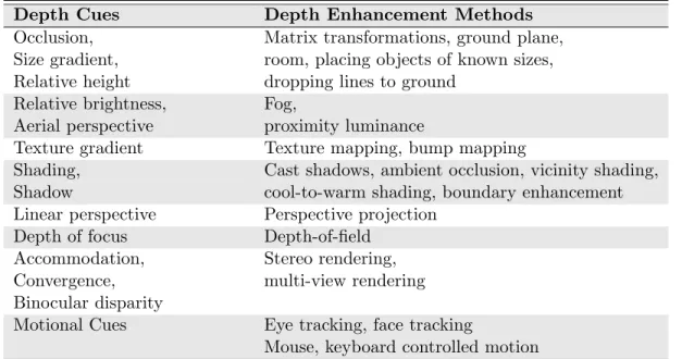
Based on the depth cues and principles discussed in the previous section, different rendering methods have been developed for enhancing depth perception in 3D rendered scenes. It is appropriate to examine these methods according to the cues they provide as listed in Table 2.1.

Perspective-based cues: It is possible to obtain the cues occlusion, size gradi-ent, and relative height by transforming the objects in the scene or changing the camera position. For the relative height cue, drawing lines from the objects to the ground plane is widely used to make the height between the object and the ground more visible [57]. A ground plane or a room facilitates the interpretation of the cues relative height and size gradient. In addition, placing objects of known sizes is a method for enabling the user to judge the sizes of unknown objects [57].

Table 2.1: Methods for enhancing depth perception, according to depth cues.

Depth Cues Depth Enhancement Methods Occlusion, Matrix transformations, ground plane, Size gradient, room, placing objects of known sizes, Relative height dropping lines to ground

Relative brightness, Fog,

Aerial perspective proximity luminance

Texture gradient Texture mapping, bump mapping

Shading, Cast shadows, ambient occlusion, vicinity shading, Shadow cool-to-warm shading, boundary enhancement Linear perspective Perspective projection

Depth of focus Depth-of-field Accommodation, Stereo rendering, Convergence, multi-view rendering Binocular disparity

Motional Cues Eye tracking, face tracking

Mouse, keyboard controlled motion

Focus related cues: Depth-of-field method is used to simulate the depth-of-focus cue. According to this method, objects in the range of focus are rendered sharp, while the objects outside of this range are rendered blurry and the blurriness level increases as the objects get further away from the range of focus [70]. Fog is commonly used to provide aerial perspective and relative brightness cues on the graphical contents and obtained by interpolating the color of a pixel between the surface color and the fog color with respect to the distance of the object. To make the relative brightness more obvious, Dosher et al. have proposed another method called proximity luminance covariance, which alters the contrast of the objects in the direction of the background color as the distance increases [57].

Shading and shadows: Several techniques have been proposed to approximate the global illumination calculation for real-time rendering. The ambient occlusion technique aims to increase the realism of 3D graphics in real time without a complete global illumination calculation. In Bunnel’s [71] work, an accessibility value, which represents the amount of hemisphere above the surface element not occluded by the geometry, is calculated by approximation for each surface

element. The surfaces are darkened according to these accessibility values.

Gooch shading is a non-photorealistic (NPR) shading model which is per-formed by interpolating between cool colors (blue tones) to warm colors (yellow tones) according to the distance from the light source [72, 73]. This kind of shading also provides atmospheric effect on the scene.

Boundary enhancement using silhouette and feature edges is a commonly-used tool in NPR [74, 75]. An image-space approach is proposed by Luft et al. [76] to enhance images that contain depth information. In this method, the difference between the original and the low-pass filtered depth buffer is computed to find spatially important areas. Then, color contrast on these areas is increased.

Binocular and oculomotor cues: To obtain binocular and oculomotor cues, there is a need for apparatus that provides multiple views of a 3D scene. There are several 3D display technologies such as shutter glasses, parallax barrier, lenticular, holographic, and head-tracked displays [77]. Rendering on 3D displays is an active topic in itself [78].

Motion related cues: Tracking the user’s position and controlling the motion of the scene elements according to the position of the user can be a tool for motion parallax. For instance, Bulbul et al. [79] propose a face tracking algorithm in which the user’s head movements control the position of the camera and enables the user to see the scene from different viewpoints.

2.2.2.2 Depth Perception in Information Visualization

Although there are a number of studies that investigate the perception of depth in scientific and medical visualizations [80, 81, 82], relatively few studies exist in the field of information visualization. The main reason behind this is that information visualization considers abstract data sets without inherent 2D or 3D semantics and therefore lacks a mapping of the data onto the physical screen space

[83]. However, when applied properly, it is hoped that using 3D will introduce a new data channel. Several applications would benefit from the visualization of 3D graphs, trees, scatter plots, etc. Earlier research claims that with careful design, information visualization in 3D can be more expressive than 2D [84]. Some common 3D information visualization methods are cone trees [85], data mountains [86], and task galleries [87]. We refer the reader to [88] and [89] for a further investigation of these techniques.

Ware and Mitchell [90] investigate the effects of binocular disparity and ki-netic depth cues for visualizing 3D graphs. They determine binocular disparity and motion to be the most important cues for graph visualization for several rea-sons. Firstly, since there are no parallel lines in graphs, perspective has no effect. Shading, texture gradient, and occlusion also have no effect unless the links are rendered as solid tubes. Lastly, shadow is distracting for large graphs. According to their experimental results, binocular disparity and motion together produce the lowest error rates. Staib et al. [91] aim improving the scatter plot visualizations by employing depth-of-field effect, depending on the area of interest.

A number of rendering methods such as shadows, texture mapping, fog, etc. are commonly used for enhancing depth perception in computer graphics and visualization. However, there is no comprehensive framework for uniting differ-ent methods of depth enhancemdiffer-ent in a visualization. A recdiffer-ent study by Hall et al. [92] present a survey about the existing emphasis frameworks for information visualization and propose a new mathematical framework for information visual-ization emphasis, based on visual prominence sets. Studies by Tarini et al. [81], Weiskopf and Ertl [93], and Swain [94] aim to incorporate several depth cues but they are limited in terms of the number of cues they consider.

Our aim is to investigate how to apply widely-used rendering methods in com-bination, to support the current visualization task. Our primary goal is to reach a comprehensible visualization in which the user is able to perform the given task easily. According to Ware [95], “depth cues should be used selectively to support design goals and it does not matter if they are combined in ways that are inconsistent with realism”. Depth cueing used in information visualization

is generally stronger than any realistic atmospheric effects, and there are several artificial techniques such as proximity luminance, dropping lines to ground plane, etc. [57]. Moreover, Kersten et al. [96] found no effect of shadow realism on depth perception. These findings show that it is possible to exaggerate the effects of these methods to obtain a comprehensible scene at the expense of deviating from realism.

Chapter 3

Visual Quality Assessment of

Dynamic Meshes

Figure 3.1: Overview of the perceptual quality evaluation for dynamic triangle meshes.

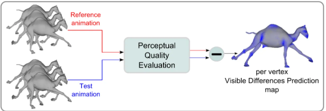
In this chapter, we propose a method to estimate the 3D spatiotemporal re-sponse, by incorporating temporal as well as spatial HVS processes. For this purpose, our method extends the image-space sensitivity models for 2D imagery in 3D space. These models, based on vast amount of empirical research on retinal images, allow us to follow a more principled approach to model the perceptual response to 3D meshes. The result of our perceptual quality metric is the prob-ability of distortion detection as a 3D map, acquired by taking the difference between estimated visual response 3D map of both meshes (Figure 3.1).

We propose two alternative methods for evaluating the perceived quality of dynamic triangle meshes. In the first approach, which we call voxel-based, we construct a 4D space-time (3D+time) volume and extend several HVS correlated processes used for 2D images, to operate on this volume. On the other hand, the second approach called mesh-based, directly operates on the mesh vertices. Following sections include detailed explanations of both methods.

3.1

Voxel-based Approach

3.1.1

Overview

Our work shares some features of the VDP method [29] and recent related work. These methods have shown the ability to estimate the perceptual quality of static images [29] and 2D video sequences for animated walkthroughs [47].

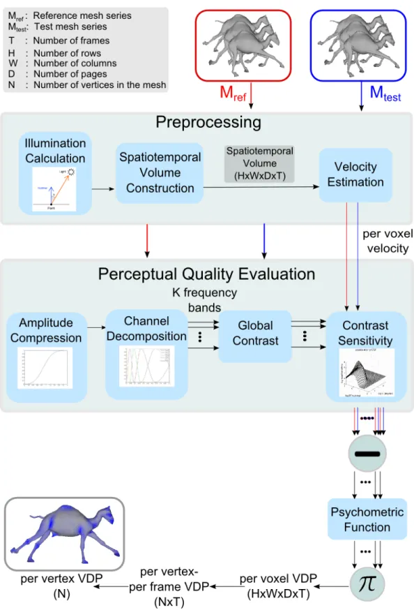
Figure 3.2 portrays the overview of the method. Our method has a full ref-erence approach in which a refref-erence and a test mesh sequence are provided to the system. Both the reference and test sequences undergo the same perceptual quality evaluation process and the difference of these outputs is used to generate a per-vertex probability map for the animated mesh. The probability value at a vertex estimates the visible difference of the distortions in the test animation, when compared to the reference animation. Below, the steps of the algorithm are explained in detail.

3.1.2

Preprocessing

Calculation of the illumination, construction of the spatiotemporal volume, and estimation of vertex velocities are performed in the preprocessing step, since we do not need to recalculate them later.

Illumination Calculation. First we calculate the vertex colors assuming a Lambertian surface with diffuse and ambient components (Eq. 3.1).

I = kaIa+ kdId(N · L) (3.1)

where Ia is the intensity of the ambient light, Id is the intensity of the diffuse

light, N is the vertex normal, L is the direction to the light source, and ka and

kd are ambient and diffuse reflection coefficients, respectively.

In this study, we aim a general-purpose quality evaluation that is independent of connectivity, shading, and material properties. Therefore, information about the material properties, light sources, etc. are not available. A directional light source from left-above of the scene is assumed in accordance with the human visual system’s assumptions [55, Section 24.4.2].

The lighting model with the aforementioned assumptions can be generalized to incorporate multiple light sources, specular reflections, etc. using Eq. 3.2; if light sources and material properties are available.

I = kaIa+ n

X

i=1

[kdIdi(N · Li) + ksIdi(N · Hi)p] (3.2)

where n is the number of light sources, ks is the specular reflection coefficient,

and H is the halfway vector.

Construction of the Spatiotemporal Volume. We convert the object-space mesh sequences into an intermediate volumetric representation, to be able to apply image-space operations. We construct a 3D volume for each frame, where we store the luminance values of the vertices at each voxel. The values of the empty voxels are determined by linear interpolation.

Using such a spatiotemporal volume representation provides an important flex-ibility as we get rid of the connectivity problems and it allows us to compare meshes with different number of vertices. Moreover, the input model is not re-stricted to be a triangle mesh; volumetric representation enables the algorithm to be applied on other representations such as point-based graphics. Another

advantage is that the complexity of the algorithm is not much affected by the number of vertices.

To obtain the spatiotemporal volume, we first calculate the Axis Aligned Bounding Box (AABB) of the mesh. To prevent inter-frame voxel correspon-dence problems, we use the overall AABB of the mesh sequences. We use the same voxel resolution for both test and reference mesh sequences. Determining the suitable resolution for the voxels is critical since it highly affects the accu-racy of the results and the time and memory complexity of the algorithm. At this point, we use a heuristic to calculate the resolution at each dimension, in proportion to the length of the bounding box in the corresponding dimension. According to this heuristic, in Eq. 3.3, we calculate the volume resolution as W , H, and D in x, y, and z dimensions respectively. We analyze the effect of the minResolution parameter in this equation on the accuracy, in the results section.

minLength = min(widthAABB, heightAABB, depthAABB)

w = bwidthAABB/minLengthc

h = bheightAABB/minLengthc

d = bdepthAABB/minLengthc

W = w × minResolution H = h × minResolution D = d × minResolution

(3.3)

At the end of this step, we obtain a 3D spatial volume for each frame, which in turn constructs a 4D (3D+time) representation for both reference and test mesh sequences. We call this structure spatiotemporal volume. Also, an index structure is maintained to keep the voxel indices of each vertex. The rest of the method operates on this 4D spatiotemporal volume.

In the following steps, we do not use the full spatiotemporal volume for perfor-mance related concerns. We define a time window as suggested by Myszkowski et al. [47, p. 362]. According to this heuristic, we only consider a limited number of consecutive frames to compute the visible difference prediction map of a specific frame. In other words, to calculate the probability map for the ith _{frame, we}

process the frames between i − btw/2c and i + btw/2c, where tw is the length of the time window. We empirically set it as tw = 3.

Velocity Estimation. Since our method also has time dimension, we need the vertex velocities in each frame. Using an index structure, we compute the voxel displacement of each vertex (Di) between consecutive frames (∆Di = kpit−

pi(t−1)k where pitdenotes the voxel position of vertex i at frame t). The remaining

empty voxels inside the bounding box are assumed to be static.

Then we calculate the velocity of each voxel at each frame (v in deg/sec), using the pixel resolution (ppd in pixels/deg) and frame rate (F P S in f rames/sec) with Eq. 3.4. We assume default viewing parameters of 0.5m viewing distance and 19-inch display with 1600X900 resolution, while calculating ppd in Eq. 3.4. This is then adapted with N1 frames to reduce the erroneous computations (Eq. 3.5).

vit =

∆Di

ppd × F P S (3.4)

v_it0 = vi(t−1)+ vit+ vi(t+1)

3 (3.5)

Lastly, it is crucial to compensate for smooth pursuit eye movements to be used in spatiotemporal sensitivity calculations. This will allow us to handle temporal masking effect where high-speed motion hides the visibility of distortions. The following equation (Eq. 3.6) describes a motion compensation heuristic proposed by Daly [54].

vR = vI− min(0.82vI+ vmin, vmax) (3.6)

where vR is the compensated velocity, vI is the physical velocity, vmin is the drift

velocity of the eye (0.15 deg/sec), vmax is the maximum velocity that the eye can

track efficiently (80 deg/sec). According to Daly [54], the eye tracks all objects in the visual field with an efficiency of 82 %. We adopt the same efficiency value for our spatiotemporal volume. However, if the visual attention map is available, it is also possible to substitute this map as the tracking efficiency [97].

3.1.3

Perceptual Quality Evaluation

In this section, the main steps of the perceptual quality evaluation system are explained in detail.

Amplitude Compression. Daly [29] proposes a simplified local amplitude non-linearity model as a function of pixel location, which assumes perfect local adap-tation (Section 2.1.2.1). We have adapted this nonlinearity to our spatiotemporal volume representation (Eq. 3.7).

R(x, y, z, t) Rmax

= L(x, y, z, t)

L(x, y, z, t) + c1L(x, y, z, t)

b (3.7)

where x, y, z, and t are voxel indices, R(x, y, z, t)/Rmaxis the normalized response,

L(x, y, z, t) is the value of the voxel, b = 0.63 and c1 = 12.6 are empirically set

constants. Voxel values are compressed by this amplitude nonlinearity.

Channel Decomposition. We have adapted the Cortex Transform [29] which is described in Section 2.1.2.2, on our spatiotemporal volume with a small exception. A 3D model is not assumed to have a specific orientation at a given time, in our method. For this purpose, we exclude fan filters that are used for orientation selectivity from the Cortex Transform adaptation. Therefore, in our cortex filter implementation we use Eq. 3.8 instead of Eq. 2.6 with only dom filters (Eq. 2.2). These band-pass filters are demonstrated in Figure 3.3.

Bk= (

domk for k = 1...K − 1

baseband for k = K (3.8) We perform cortex filtering in the frequency domain by applying Fast Fourier Transform (FFT) on the spatiotemporal volume and multiplying this with the cortex filters that are constructed in the frequency domain. We obtain K fre-quency bands at the end of this step. Each frefre-quency band is then transformed back to the spatial domain using Inverse Fourier Transform. This process is illustrated in Figure 3.4.

Global Contrast. The sensitivity to a pattern is determined by its contrast rather than its intensity [98]. Contrast in every frequency channel is computed

Figure 3.3: Difference of Mesa (DOM) filters. (x-axis: spatial frequency in cycles/pixel, y-axis: response)

according to the global contrast definition with respect to the mean value of the whole channel, given in Eq. 3.9 [98, 47].

Ck = I

k_{− mean(I}k₎

mean(Ik₎ (3.9)

where Ckis the spatiotemporal volume of contrast values and Ikis the spatiotem-poral volume of luminance values in channel k.

Contrast Sensitivity. Filtering the input image with the Contrast Sensitiv-ity Function (CSF) constructs the core part of the VDP-based models (Section 2.1.2.3). Since our model is for dynamic meshes, we use the spatiovelocity CSF (Figure 2.5b) which describes the variations in visual sensitivity as a function of both spatial frequency and velocity, instead of the static CSF used in the original VDP.

Our method handles temporal distortions in two ways: First, smooth pursuit compensation handles temporal masking effect which refers to the loss of sensi-tivity due to high speed. Secondly, we use spatiovelocity CSF in which contrast sensitivity is measured according to the velocity, instead of static CSF.

Each frequency band is weighted with the spatiovelocity CSF which is given in Eq. 3.10 [54, 53]. One input to the CSF is per voxel velocities in each frame, estimated in preprocessing; and the other input is the center spatial frequency of

Figure 3.4: Frequency domain filtering in Cortex Transform.

each frequency band.

CSF (ρ, v) = c0(6.1 + 7.3| log( c2v 3 ) | 3 ) × c2v(2πc1ρ)2× exp(− 4πc1ρ(c2v + 2) 45.9 ) (3.10) where ρ is the spatial frequency in cycles/degree, v is the velocity in degrees/second, and c0 = 1.14, c1 = 0.67, c2 = 1.7 are empirically set

coeffi-cients. A more principled way would be to obtain these parameters through a parameter learning method.

Error Pooling. All the previous steps are applied on the reference and test animations. At the end of these steps, we obtain K channels for each mesh sequence. We take the difference of test and reference pairs for each channel and the outputs go through a psychometric function that maps the perceived contrast (C0) to detection probability using Eq. 3.11 [43]. After applying the psychometric function, we combine each band using the probability summation formula (Eq. 3.12) [43].

ˆ P = 1 − K Y k=1 (1 − Pk) (3.12)

The resulting ˆP is a 4D volume that contains the detection probabilities per voxel. It is then straightforward to convert this 4D volume to per vertex probability map for each frame, using the index structure (Section 3.1.2). Lastly, to combine the probability maps of each frame into a single map, we take the average of all frames per vertex. This gives us a per vertex visible difference prediction map for the animated mesh.

Summary of the Method. The overall process is summarized in Eq.3.13 in which F denotes the Fourier Transform, F−1 denotes the Inverse Fourier Trans-form, and LT and LR are spatiotemporal volumes for test and reference mesh

sequences, respectively. ρk _{is the center spatial frequency of channel k and V} T

and VR contain the voxel velocities corresponding to LT and LR respectively.

C_T,Rk = Contrast(Channel_{T ,R}k ) × CSF (ρk, VT,R)

Channelk_{T ,R}= F−1[F (ACT ,R) × DOMk]

ACT ,R= AmplitudeCompression(LT ,R) Pk = P (C_Tk− Ck R) P = 1 − K Y k=1 (1 − Pk) (3.13)

3.2

Mesh-based Approach

Due to the limitations such as computational complexity of the voxel-based ap-proach, we also propose a fully mesh-based method as an alternative. In this method, we benefit from the eigen-decomposition of a mesh since eigenvalues are identified as natural vibrations of a mesh [99, Chapter 4] and hence, they are directly related to the geometric quality of the mesh.

3.2.1

Overview

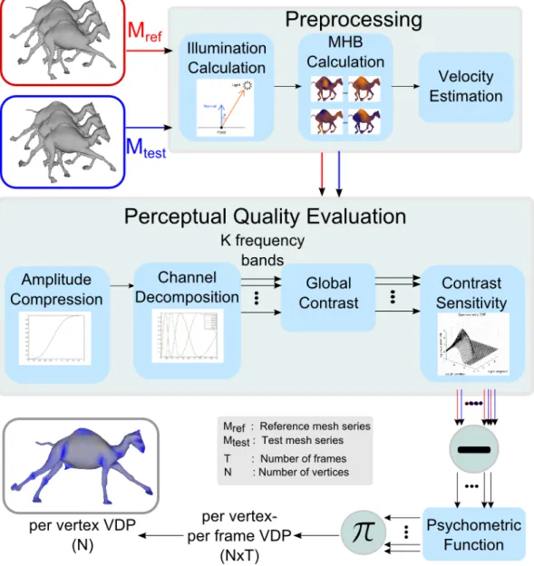
In this mesh-based approach, almost the same steps in the voxel-based approach exist with several adaptations for 3D. The method is applied on the mesh vertices, not on the spatiotemporal volume representation. However, this introduces a restriction for the reference and test meshes to have the same number of vertices, since the computations are done per vertex. The steps of the method are displayed in Figure 3.5. Only the different parts of the algorithm will be described in detail.

3.2.2

Preprocessing

In the preprocessing step, illumination calculation and vertex velocity estima-tion are performed as in the voxel-based approach. The spatiotemporal volume construction step is not executed this time, since the rest of the algorithm will operate on the mesh vertices. As an additional step, Manifold Harmonics Basis (MHB) are computed and stored to feed the Channel Decomposition step of the new approach.

Calculation of MHBs. Calculation of MHBs is a costly operation since it requires eigen-decomposition of the mesh Laplacian. Fortunately, once they are computed; there is no need to recalculate them. Therefore, we calculate and store the MHBs in the preprocessing step.

For a triangle mesh of n vertices, a function basis Hk_{, called MHB is calculated.}

The kth_{element of the MHB is a piecewise linear function with values H}k

i defined

at ith_{vertex of the surface, where k = 1...m and i = 1...n [100]. MHB is computed}

as the eigenvectors of discrete Laplacian of ¯∆ whose coefficients are given in Eq. 3.14. ¯ ∆ij = − cotβij + cotβij0 q |v∗ i||vj∗| (3.14)

where βij and βij0 are two angles opposite to edge defined by vertices i and j, v ∗

3.2.3

Perceptual Quality Evaluation

All the steps of this method are similar to the corresponding steps in the voxel-based approach. Therefore, only Channel Decomposition step which is totally different from its counterpart in the previous approach will be explained in detail. Other steps follow the same procedures described in the previous section, with the exception that equations are applied per vertex instead of per voxel, since they are not applied on the spatiotemporal volume.

Channel Decomposition. The most important distinction of the mesh-based approach lies in the Channel Decomposition step. In this step of the voxel-based approach, we use Cortex Transform which filters the spatiotemporal volume with DoM (Difference Of Mesa) filters in the frequency domain. Manifold Harmonics can be considered as the generalization of Fourier analysis to surfaces of arbitrary topology [100]. Hence, we employ Manifold Harmonics for applying DoM filter on the mesh and obtain 6 frequency channels as in the voxel-based approach.

Figure 3.6 demonstrates the processing pipeline of Manifold Harmonics. In step A of this pipeline, Manifold Harmonics Basis is calculated for the given triangle mesh of N vertices, which is already performed in the preprocessing step in our implementation.

Figure 3.6: Pipeline for Manifold Harmonics Transform. (Image from [100], c 2008 John Wiley and Sons, reprinted with permission.)