A Novel STFT Implementation for the Analysis of Non-Stationary
Jammer Interference
Lutfiye Durak∗, Orhan Arikan∗∗, and Iickho Song∗ ∗Department of Electrical Engineering
Korea Advanced Institute of Science and Technology 373-1 Guseong Dong, Yuseong Gu, Daejeon 305-701, Korea
[email protected], [email protected]
∗∗Department of Electrical Engineering
Bilkent University Ankara, 06800, Turkey [email protected]
ABSTRACT
A novel adaptive short-time Fourier transform (STFT) implementation for the analysis of non-stationary multi-component jammer signals is introduced. The pro-posed time-frequency distribution is the fusion of optimum STFTs of individual signal components that are based on the recently introduced generalized time-bandwidth prod-uct (GTBP) definition. The GTBP optimal STFTs of the components are combined through thresholding and ob-taining the individual component support images, which are related with the corresponding GTBP optimal STFTs.
KEY WORDS
Non-stationary signal analysis, linear time-frequency dis-tributions, short-time Fourier transform, generalized time-bandwidth product, multi-component chirp jammers.
1
Introduction
Spread spectrum techniques inherently provide resistance to jammer interference by the despreading gain. However, if the interference is much stronger than the desired signal, the gain becomes insufficient to decode the signal reliably. This is the case when interference stations are much closer to the receiver than the transmitter, or the transmitted sig-nal is affected by fading. Therefore, in spread spectrum communications, several interference excision techniques are employed to improve the receiver performance and re-duce the bit error rates including adaptive filtering, trans-form domain methods and time-frequency analysis tech-niques [1–4]. In particular, the non-stationary interfer-ence mitigation of chirp jammers is based on the time-frequency distributions of the short-time Fourier transfor-mation (STFT) as in [3] or the Wigner distribution (WD) as in [1]. The chirp jammers have wideband frequency characteristics with narrow instantaneous bandwidth and the interference is suppressed once the jammer
characteris-tics are identified by using the time-frequency distributions. This is achieved either by masking out the jammer from the 2-D STFT followed by the synthesis of the jammer-free signal [3] or by adaptive time-varying filtering where the parameters of the interfering signal is estimated from the WD [5].
In both of these interference excision techniques, in-herent drawbacks of the time-frequency distributions limit the system performance. An important criterion for the success of time-frequency representations is how well it preserves the time-frequency domain support of signals. Among the commonly used time-frequency representa-tions, WD is the best in this respect. However, since the WD is a quadratic time-frequency distribution, in the case of multi-component signals, the cross-terms of the WD clutters the obtained time-frequency representation. There-fore, in a way it disturbs the actual support of the signal in the time-frequency domain. The linear STFT family pro-vides time-frequency representations without cross-terms, but poor time-frequency localization of signal components is the major drawback of the STFT.
Recently, by investigating the effect of the STFT kernel on the time-frequency support of signal compo-nents, an optimal STFT implementation based on a novel generalized time-bandwidth product (GTBP) is proposed in [6]. The computationally efficient optimal STFT pro-vides the most compact representation of single compo-nent signals considering their GTBP and yields optimally compact time-frequency supports for chirp signals on the STFT plane. In this paper, the GTBP optimal STFT im-plementation is extended for multi-component signals and it is proposed as a powerful analysis tool of spread spec-trum communication applications in the presence of multi-component chirp jammers.
2
Time-Frequency Localization by STFT
The discrete STFT of a signalx(t) is defined as1[7]
STFTx(nT, mF ) = Z x(t′)g∗(t′ − nT )e−2πmF t ′ dt′ ≃ T X n′ x(n′T)g∗(n′ T − nT )e−2πmF n′T , (1)
whereg(.) is the kernel function, n, m, n′are integers, and
T and F are the sampling intervals of time and frequency. By using the FFT techniques, (1) can be implemented effi-ciently.
The choice of the STFT kernel g(t) determines the time-frequency signal localization properties of the dis-tribution. The Gaussian function is the most commonly used kernel function because it has the minimum time-bandwidth product (TBP), which is defined as
TBP{x(t)} = Tx· Bx, (2)
whereTx andBx are the time-width and bandwidth of a
signalx(t). The TBP has been commonly used as a mea-sure for the time-frequency domain support of the signal. The well-known uncertainty principle dictates that1/(4π) is a lower bound on the TBP of a signal and only the Gaus-sian signal has a TBP that is equal to this lower bound [8]. For an STFT kernel functiong(t), the time-frequency domain support of the representation of a signalx(t) can be zoned into a rectangular region with time and frequency dimensionsqT2
x+ Tg2and
q
B2
x+ B2g, respectively [9].
Therefore, if the TBP is chosen as the measure of sup-port, a well-defined optimization problem can be cast for the optimal STFT kernel, and the TBP optimal STFT
ker-nelgT BP(t) is derived as [10]
gT BP(t) = e−πt
2Bx/Tx
. (3)
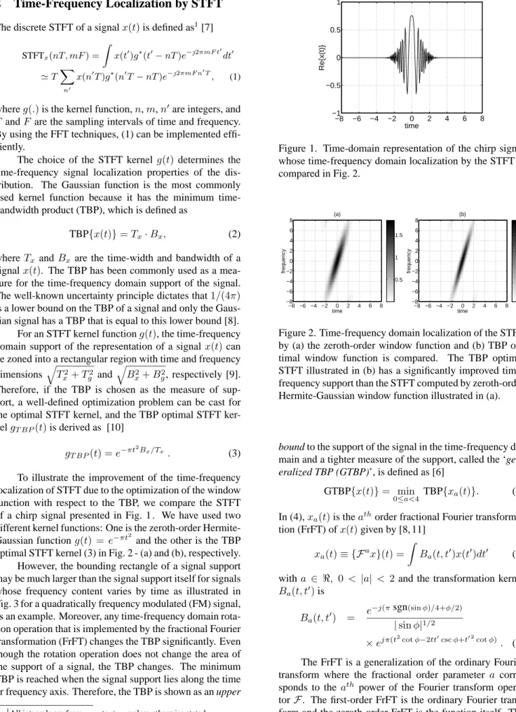
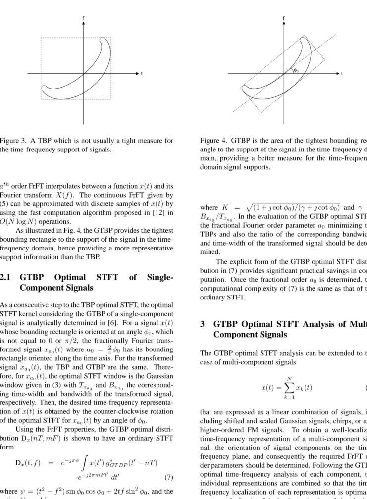
To illustrate the improvement of the time-frequency localization of STFT due to the optimization of the window function with respect to the TBP, we compare the STFT of a chirp signal presented in Fig. 1 . We have used two different kernel functions: One is the zeroth-order Hermite-Gaussian functiong(t) = e−πt2
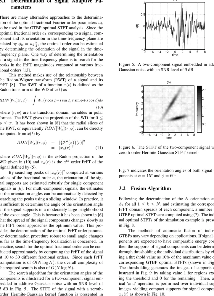
and the other is the TBP optimal STFT kernel (3) in Fig. 2 - (a) and (b), respectively. However, the bounding rectangle of a signal support may be much larger than the signal support itself for signals whose frequency content varies by time as illustrated in Fig. 3 for a quadratically frequency modulated (FM) signal, as an example. Moreover, any time-frequency domain rota-tion operarota-tion that is implemented by the fracrota-tional Fourier transformation (FrFT) changes the TBP significantly. Even though the rotation operation does not change the area of the support of a signal, the TBP changes. The minimum TBP is reached when the signal support lies along the time or frequency axis. Therefore, the TBP is shown as an upper
1All integrals are from −∞ to +∞ unless otherwise stated.
−8 −6 −4 −2 0 2 4 6 8 −1 −0.5 0 0.5 1 time Re{x(t)}
Figure 1. Time-domain representation of the chirp signal whose time-frequency domain localization by the STFT is compared in Fig. 2. 0.5 1 1.5 time frequency (a) −8 −6 −4 −2 0 2 4 6 8 −8 −6 −4 −2 0 2 4 6 8 0 0.5 1 1.5 2 time frequency (b) −8 −6 −4 −2 0 2 4 6 8 −8 −6 −4 −2 0 2 4 6 8
Figure 2. Time-frequency domain localization of the STFT by (a) the zeroth-order window function and (b) TBP op-timal window function is compared. The TBP optimal STFT illustrated in (b) has a significantly improved time-frequency support than the STFT computed by zeroth-order Hermite-Gaussian window function illustrated in (a).
bound to the support of the signal in the time-frequency do-main and a tighter measure of the support, called the ‘gen-eralized TBP (GTBP)’, is defined as [6]
GTBP{x(t)} = min
0≤a<4 TBP{xa(t)}. (4)
In (4),xa(t) is the athorder fractional Fourier
transforma-tion (FrFT) ofx(t) given by [8, 11]
xa(t) ≡ {Fax}(t) =
Z
Ba(t, t′)x(t′)dt′ (5)
witha ∈ ℜ, 0 < |a| < 2 and the transformation kernel
Ba(t, t′) is
Ba(t, t′) =
e−j(πsgn(sin φ)/4+φ/2)
| sin φ|1/2
× ejπ(t2cot φ−2tt′csc φ+t′ 2cot φ). (6) The FrFT is a generalization of the ordinary Fourier transform where the fractional order parameter a corre-sponds to the ath power of the Fourier transform
opera-torF. The first-order FrFT is the ordinary Fourier
f
t
Figure 3. A TBP which is not usually a tight measure for the time-frequency support of signals.
athorder FrFT interpolates between a functionx(t) and its
Fourier transformX(f ). The continuous FrFT given by (5) can be approximated with discrete samples ofx(t) by using the fast computation algorithm proposed in [12] in O(N log N ) operations.
As illustrated in Fig. 4, the GTBP provides the tightest bounding rectangle to the support of the signal in the time-frequency domain, hence providing a more representative support information than the TBP.
2.1
GTBP
Optimal
STFT
of
Single-Component Signals
As a consecutive step to the TBP optimal STFT, the optimal STFT kernel considering the GTBP of a single-component signal is analytically determined in [6]. For a signalx(t) whose bounding rectangle is oriented at an angleφ0, which
is not equal to 0 or π/2, the fractionally Fourier trans-formed signal xa0(t) where a0 = π2φ0 has its bounding
rectangle oriented along the time axis. For the transformed signalxa0(t), the TBP and GTBP are the same.
There-fore, forxa0(t), the optimal STFT window is the Gaussian
window given in (3) withTxa0 andBxa0 the
correspond-ing time-width and bandwidth of the transformed signal, respectively. Then, the desired time-frequency representa-tion ofx(t) is obtained by the counter-clockwise rotation of the optimal STFT forxa0(t) by an angle of φ0.
Using the FrFT properties, the GTBP optimal distri-bution Dx(nT, mF ) is shown to have an ordinary STFT
form Dx(t, f ) = e−πψ Z x(t′) g∗ GT BP(t′− nT ) ·e−2πmF t′ dt′ (7) whereψ = (t2− f2) sin φ
0cos φ0+ 2tf sin2φ0, and the
optimal kernel is gGT BP(τ ) = K e −πτ2 cot φ0(γ2−1) γ2+cot2 φ0 e−πτ 2 γcsc2 φ0 γ2+cot2 φ0 (8) f t φ0
Figure 4. GTBP is the area of the tightest bounding rect-angle to the support of the signal in the time-frequency do-main, providing a better measure for the time-frequency domain signal supports.
where K = p(1 + cot φ0)/(γ + cot φ0) and γ =
Bxa0/Txa0. In the evaluation of the GTBP optimal STFT,
the fractional Fourier order parametera0 minimizing the
TBPs and also the ratio of the corresponding bandwidth and time-width of the transformed signal should be deter-mined.
The explicit form of the GTBP optimal STFT distri-bution in (7) provides significant practical savings in com-putation. Once the fractional ordera0 is determined, the
computational complexity of (7) is the same as that of the ordinary STFT.
3
GTBP Optimal STFT Analysis of
Multi-Component Signals
The GTBP optimal STFT analysis can be extended to the case of multi-component signals
x(t) =
N
X
k=1
xk(t) (9)
that are expressed as a linear combination of signals, in-cluding shifted and scaled Gaussian signals, chirps, or any higher-ordered FM signals. To obtain a well-localized time-frequency representation of a multi-component sig-nal, the orientation of signal components on the time-frequency plane, and consequently the required FrFT or-der parameters should be determined. Following the GTBP optimal time-frequency analysis of each component, the individual representations are combined so that the time-frequency localization of each representation is optimally compact. In Section 3.1, the determination of signal adap-tive parameters are explained. The fusion algorithm is de-scribed in Section 3.2.
3.1
Determination of Signal Adaptive
Pa-rameters
There are many alternative approaches to the determina-tion of the optimal fracdetermina-tional Fourier order parametersak
to be used in the GTBP optimal STFT analysis. Since the optimal fractional orderakcorresponding to a signal
com-ponent and its orientation in the time-frequency plane are related byφk = akπ2, the optimal order can be estimated
by determining the orientation of the signal in the time-frequency plane. One way of determining the orientation of a signal in the time-frequency plane is to search for the peaks in the FrFT magnitudes computed at various frac-tional orders [13].
This method makes use of the relationship between the Radon-Wigner transform (RWT) of a signal and its FrFT [8]. The RWT of a function x(t) is defined as the Radon transform of the WD ofx(t) as
RDN[Wx](r, φ) =
Z
Wx(r cos φ−s sin φ, r sin φ+s cos φ)ds
(10)
where(r, φ) are the transform domain variables in polar format. The RWT gives the projection of the WD for0 ≤ φ ≤ π. It has been shown in [8] that the radial slices of the RWT, or equivalentlyRDN [Wx](r, φ), can be directly
computed fromx(t) by
RDN [Wx](r, φ) = |{Fa(x)}(r)|2
= |xa(r)|2 (11)
whereRDN [Wx](r, φ) is the φ-Radon projection of the
WD given in (10) andxa(r) is the athorder FrFT of the
signal defined by (5).
By searching peaks of|xa(r)|2 computed at various
values of the fractional ordera, the orientation of the sig-nal supports are estimated robustly for single component signals in [6]. For multi-component signals, the estimates of the orientation angles can be automatically detected by searching the peaks using a sliding window. In practice, it is sufficient to determine the angle of the orientation angle of the signal supports in a moderately large neighborhood of the exact angle. This is because it has been shown in [6] that the spread of the signal components changes slowly as the FrFT order approaches the optimum value. This pro-vides the determination of the optimal FrFT order parame-ter deparame-termination procedure robust to small angle changes as far as the time-frequency localization is concerned. In practice, search for the optimal fractional order can be con-ducted approximately by computing the FrFT of the signal at 10 to 30 different fractional orders. Since each FrFT computation is of O(N log N ), the overall complexity of the required search is also ofO(N log N ).
The search algorithm for the orientation angles of the components is illustrated for a two-component signal em-bedded in additive Gaussian noise with an SNR level of 5 dB in Fig. 5 . The STFT of the signal with a zeroth-order Hermite-Gaussian kernel function is presented in Fig. 6. The projection analysis using the FrFT presented in
−8 −6 −4 −2 0 2 4 6 8 −1 −0.5 0 0.5 1 time x(t) (a)
Figure 5. A two-component signal embedded in additive Gaussian noise with an SNR level of 5 dB.
time frequency (b) −8 −6 −4 −2 0 2 4 6 8 −8 −6 −4 −2 0 2 4 6 8 0.5 1 1.5 2 2.5
Figure 6. The STFT of the two-component signal with a zeroth-order Hermite-Gaussian STFT kernel.
Fig. 7 indicates the orientation angles of both signal com-ponents atφ = 15◦andφ = 60◦.
3.2
Fusion Algorithm
Following the determination of the N orientation angles φk for all1 ≤ k ≤ N , and estimating the corresponding
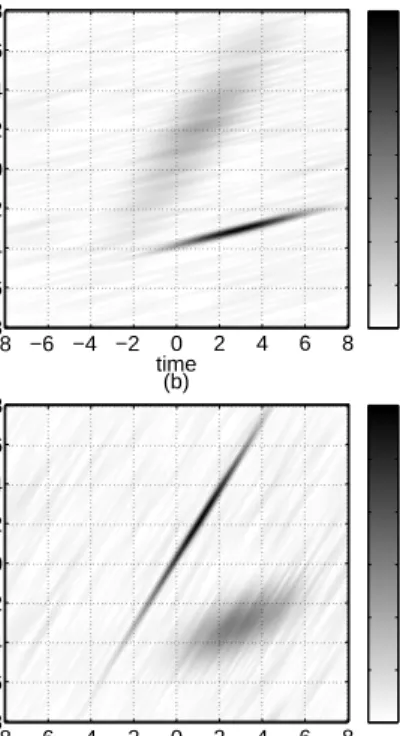
FrFT domain spreads of each component, a number ofN GTBP optimal STFTs are computed using (7). The individ-ual optimal STFTs of the simulation example is presented in Fig. 8.
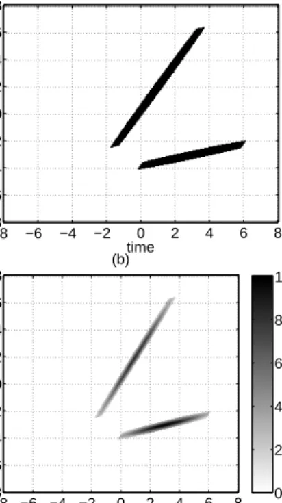
The methods of automatic fusion of individual GTBPs may vary depending on applications. If signal com-ponents are expected to have comparable energy content, then the supports of signal components can be determined through thresholding the individual distributions by choos-ing a threshold value as 10% of the maximum value of the corresponding GTBP optimal STFTs (shown in Fig. 8 ). The thresholding generates the images of supports as il-lustrated in Fig. 9 by taking value 1 for regions exceed-ing the threshold and 0 for the remainexceed-ing. Then, a log-ical ‘and’ operation is performed over individual support images yielding compact supports for signal components
xk(t) as shown in Fig. 10.
−901 −60 −30 0 30 60 90 1.5 2 2.5 3 φ − π/2
Peak amplitude of the FrFT
(c)
Figure 7. By searching peaks of the|xa(r)|2signals
com-puted at variousa values, the orientation of the signal sup-ports can be estimated robustly. The projection analysis us-ing the FrFT is presented indicatus-ing the orientation angles of both signal components atφ = 15◦andφ = 60◦.
supports can be matched to the individual GTBP optimal STFTs by taking into account of the component energy en-capsulated by the support. In Fig. 10(a) and (b), the final support and the resultant adaptive STFT is presented. Al-ternatively, watershed segmentation algorithm can be used in the automatic determination of the supports of individual components [14].
The time-frequency localization of each signal com-ponent is significantly improved compared to the STFT in Fig. 6 . In spread spectrum communication applications, the interference excision can be performed by masking out the high-power jammer signal supports and synthesize the jammer-free signal from the remaining time-frequency dis-tribution.
4
Conclusion
In this paper, the recently developed optimal STFT im-plementation based on the minimum TBP is extended to signals with multi-components. The GTBP optimal STFT analysis of each signal component provides a significant improvement for the time-frequency localization compared to the ordinary STFT analysis with a similar computational complexity.
The proposed GTBP optimal STFT of multi-component signals requires the determination of the param-eters of individual signal components. In practical appli-cations, these parameters should be adaptively chosen and comparison of the performances of alternative ways of de-termining these parameters requires further investigation.
Compared to the previously developed STFT-based interference excision system in [3], the proposed adaptive STFT is computationally efficient. Additionally, compared to the WD based higher-order time-frequency distributions, which retain cross-terms, this algorithm is robust. There-fore, it can be implemented in the interference excision techniques in the presence of multi-component jammers.
1 2 3 4 5 6 7 time frequency (a) −8 −6 −4 −2 0 2 4 6 8 −8 −6 −4 −2 0 2 4 6 8 1 2 3 4 5 6 time frequency (b) −8 −6 −4 −2 0 2 4 6 8 −8 −6 −4 −2 0 2 4 6 8
Figure 8. GTBP optimal STFTs associated with each signal component of the signal illustrated in Fig. 5.
Acknowledgement
This research was supported by Brain Korea 21 Project un-der a 2004 grant from the School of Information Technol-ogy, KAIST, for which the authors would like to express their thanks.
References
[1] M. G. Amin, “Interference mitigation in spread spec-trum communication systems using time-frequency distributions,” IEEE Trans. Signal Process., vol. 45, pp. 90–101, Jan. 1997.
[2] J. Laster and J. Reed, “Interference rejection in dig-ital wireless communication,” IEEE Signal Process. Magazine, vol. 14, pp. 37–62, May 1997.
[3] X. Ouyang and M. G. Amin, “Short-time Fourier transform receiver for nonstationary interference ex-cision in direct sequence spread spectrum communi-cations,” IEEE Trans. Signal Process., vol. 49, pp. 851–863, Apr. 2001.
[4] J. Yuan and J. Lee, “Narrow-band interference re-jection in DS/CDMA systems using adaptive (QRD-LSL)-Based Nonlinear ACM Interpolators,” IEEE Trans. Vehicular Tech., vol. 52, pp. 374–379, May 2003.
time frequency (a) −8 −6 −4 −2 0 2 4 6 8 −8 −6 −4 −2 0 2 4 6 8 time frequency (b) −8 −6 −4 −2 0 2 4 6 8 −8 −6 −4 −2 0 2 4 6 8
Figure 9. The supports of the signal components can be determined through thresholding the individual distribu-tions by choosing a threshold value as 10% of the maxi-mum value of the corresponding GTBP optimal STFTs il-lustrated in Fig. 8. Thresholding generates the images of supports by taking value 1 for regions exceeding the thresh-old and 0 for the remaining.
[5] S. Barbarossa and A. Scaglione, “Adaptive time-varying cancellation of wideband interferences in spread-spectrum communications based on time-frequency distributions,” IEEE Trans. Signal Pro-cess., vol. 47, pp. 957–965, Apr. 1999.
[6] L. Durak and O. Arıkan, “Short-time Fourier Trans-form: Two fundamental properties and an optimal im-plementation,” IEEE Trans. Signal Process., vol. 51, pp. 1231–1242, May 2003.
[7] F. Hlawatsch and G. F. Boudreaux-Bartels, “Linear and quadratic time–frequency signal representations,” IEEE Signal Process. Magazine, vol. 9, pp. 21–67, Apr. 1992.
[8] H. M. Ozaktas, Z. Zalevsky, and M. A. Kutay, The Fractional Fourier Transform with Applications in Optics and Signal Processing, John Wiley & Sons, 2000.
[9] L. Cohen, Time–Frequency Analysis, Prentice Hall, 1995.
[10] L. Durak and O. Arıkan, “Generalized time-bandwidth product optimal short-time Fourier trans-formation,” Proc. IEEE Int. Conf. Acoust. Speech,
time frequency (a) −8 −6 −4 −2 0 2 4 6 8 −8 −6 −4 −2 0 2 4 6 8 0 2 4 6 8 10 time frequency (b) −8 −6 −4 −2 0 2 4 6 8 −8 −6 −4 −2 0 2 4 6 8
Figure 10. Fusion of the individual GTBP optimal STFTs of multi-component signals. In (a), a logical ‘and’ opera-tion is performed over individual support images yielding compact supports for each signal component. Finally, in (b) the components corresponding to the final supports are matched to the individual optimal STFTs
Signal Process., Orlando, USA, vol. 2, pp. 1465– 1468, May 2002.
[11] V. Namias, “The fractional order Fourier trans-form and its application to quantum mechanics,” J. Inst. Math. Appl., vol. 25, pp. 241–265, 1980. [12] H. M. Ozaktas, O. Arıkan, M. A. Kutay, and
G. Bozdagi, “Digital computation of the fractional Fourier transform,” IEEE Trans. Signal Process., vol. 44, pp. 2141–2150, Sept. 1996.
[13] A. W. Lohmann and B. H. Soffer, “Relationships between the Radon–Wigner and fractional Fourier transforms,” J. Opt. Soc. Am. A, vol. 11, pp. 1798– 1801, June 1994.
[14] L. Vincent and P. Soille, “Watersheds in digital spaces: An efficient algorithm based on immersion simulations,” IEEE Trans. Pattern Analysis, Machine Intelligence, vol. 13, pp. 583–598, June 1991.