f r j : í P ±
LEÍ E'BGtESSíMn К
' , Ч ' '■ /У
"." ·ϋ*··. ^
ν' *·^ “'/»!·’“• İ.İ' «'4ИИ>/ . W· ■<
RADIOSITY
A THESIS
SUBMITTED TO THE DEPARTMENT OF COMPUTER ENGINEERING AND INFORMATION SCIENCE AND THE INSTITUTE OF ENGINEERING AND SCIENCE
OF BILKENT UNIVERSITY
IN PARTIAL FULFILLMENT OF THE REQUIREMENTS FOR THE DEGREE OF
MASTER OF SCIENCE
By
Tolga K. Çapın
September, 1993
.... tul C.I ... V.-.İ7
Д
I 9 S 2 .
ь
I
certify that I have read this thesis and that in my opinion it is fully adequate, in scope and in qiuility, as a thesis for the degree of Master of Science.Asst. Prof.^^^^let Aykanat (Advisor)
1 certify that I have read this thesis and that in my opinion it is fully adequate, in scope and in quality, as a thesis for the degree, of Master of Science.
Prof. Bülent Ozgüç
I certify that I have read this thesis and that in my opinion it is fully adequate, in scope and in quality, as a thesis for the degree of Master of Science.
Vis. Assoc
Co/^ _______ oc. Prof. Fazh Can
Approved for the Institute of Engineering and Science:
Prof. Mehme|<^aTay Director of the Institute
ABSTRACT
PARALLEL PROCESSING FOR PROGRESSIVE
REFINEMENT RADIOSITY
Tolga K . Çapın
M .S . in Computer Engineering and Information Science
Advisor: A sst. Prof. Cevdet Aykanat
September, 1993
Progressive refinement radiosity is an increasingly popular method for re alistic image synthesis of non-existing environments. The method successfully approximates the light distribution in an environment, however it requires excessive amount of computation. In this thesis, the progressive refinement method is investigated for parallelization on ring and hypercube-connected multicomputers. Two different approaches for parallelization, based on syn chronous parallelism witli static task assignment, are proposed, in order to achieve better coherence in parallel light distributions and obtain good perfor mance on simple topologies. Efficient global circulation schemes are proposed in order to decrease the total volume of communication by asymptotical fac tors. The first scheme for parallelization is a modification of the sequential algorithm in that several patches shoot their energy at a time, while the sec ond scheme is based on the parallelism level of one shooting patch at a time. The proposed parallel algorithms are evaluated theoretically and implemented for ring and hypercube-connected topologies on Intel’s iPSC72 multicomputer. Load balance quality of the proposed schemes are evaluated experimentally.
Keywords:
Realistic Image .Synthesis, Parallel Computing, Multicomputers, Radiosity, Progressive Refinement Radiosity, Ring Interconnection Topology, Hypercube Interconnection Topology.DERECELİ GELİŞEN IŞIMA İÇİN PARALEL İŞLEME
Tolga K . Çapın
Bilgisayar ve Eııfonııatik Mühendisliği, Yüksek Lisans
Danışm an: Yrd. Doç. Dr. Cevdet Aykanat
Eylül, 1993
Dereceli gelişen ışıma gerçeğe uygun görüntü üretmek için gittikçe daha fazla kullanılmakta olan bir yöntemdir. Yöntem, ışığın sahnede dağılımını başarılı bir şekilde hesaplamakta, ancak çok fazla işlem gerektirmektedir. Bu tezde, dereceli gelişen ışıma yönteminin zincir ve hiperküp bağlantılı dağıtık hafızalı çok işlemciler üzerinde paralel hesaplanması araştırılmaktadır. İşık dağılımının sırasının sağlanması ve basit topolojilerde iyi perfor mans sağlanabilmesi için eşzamanlı paralel işlemeye dayalı iki yaklaşım geliştirilmiştir. Toplam iletişim miktarını asimtotik olarak azaltmak için ve rimli dolaştırma yöntemleri önerilmiştir. Önerilen ilk paralel yaklaşım, tek- işlemcili algoritmaya değişiklik getirmiştir, çünkü bu yaklaşımda aynı anda birden fazla yüzey ışık yayar, ikinci yaklaşım aynı anda sadece bir yüzey yayıcı yöntemine göre tasarlanmıştır. Önerilen yöntemler zincir ve hiper-küp bağlantılı dağıtık hafızalı çok işlemciler için hiperküp bağlantılı Intel iP S C /2 bilgisayarında gerçekleştirilmiştir. Önerilen yöntemlerin iş dağılımı kalitesi deneysel olarak gözlenmiştir.
Anahtar Sözcükler:
Gerçeğe Uygun Görüntü , Üretme, Paralel işleme, Dağıtık Hafızalı Çok İşlemciler, Işıma, Dereceli Gelişen Işıma, Zincir Bağlantılı Topoloji, Hiperküp Bağlantılı Topoloji.ACKNOWLEDGMENTS
I would like to express my deep gratitude to my supervisor Asst. Prof. Cevdet Aykanat for his guidance, suggestions, and invaluable encouragement through out the development of this thesis.
I would also like to thank Prof. Bülent Özgüç and Assoc. Prof. Fazlı Can for reading and commenting on the thesis.
I would like to acknowledge Guy Moreillon for his house interior model. Bilge Erkan for her glass model, and Aydın Ramazanoglu for photographing the final images.
I am grateful to the members of my family and Meltem for tlieir infinite moral support and patience that they have shown, particularly in times I was not with them.
1 Introduction 1 1.1 Overview... 1 1.2 Progressive Refinement R a d io s it y ... 2 1.3 M otivation... 3 1.4 Outline of the T h e s i s ... 4 2 Radiosity 5 2.1 Realistic Image Generation... 5
2.2 The Radiosity M e t h o d ... 7
2.2.1 Form-Factor D efin ition ... 9
2.2.2 Form-Factor Computation: Hemicube M e t h o d ... 10
2.3 Progressive Refinement R a d io s it y ... 16
2.3.1 Simultaneous Update of Patch Radiosities: Shooting vs. G a th e rin g ... 17
2.3.2 Solving in Sorted Order
· · · ■ , ,
... 2.3.3 The Ambient T e r m ... 182.4 Further Improvements of the M e t h o d ... 20
2.5 Conclusion and S u m m a r y ... 25
3 Overview of Parallelism in Radiosity 26
3.1 Clcissification of Parallel A r c h ite c tu r e s ... 26
3.2 Design Criteria for Parallelization... 28
3.2.1 Type of parallelism ... 29
3.2.2 Load B a la n c in g ... 29
3.2.3 G r a n u la r ity ... 30
3.2.4 Exploiting Graphical C oh eren ce... 30
3.2.5 Data A c c e s s ... 30
3.2.6 S calab ility... 31
3.3 Parallelism in Radiosity and Previous W o r k ... 31
3.3.1 Parallelization: More than One Patch at a T i m e ... 32
3.3.2 Parallelization: One Patch at a T i m e ... 36
3.4 Critical Issues of the iP S C /2 H y p e r c u b e ... 38
3.4.1 Embedding the ring onto hypercube... 40
4 Parallelization: Patch Data Circulation 43 4.1 Introduction...43
4.2 Parallelization... 45
4.2.1 Phase 1: Shooting Patch Selection... 46
4.2.2 Phase 2: Hemicube P r o d u c t io n ... 51
4.2.3 Phase 3: Form-Factor Vector, C om p u tation ... 61
4.2.4 Phase 4: Contribution Computation ... 61
4.3 Experimental R e su lts... 67
4.4 Conclusion... 77
5 Parallelization: Hemicube M erging 78 5.1 Preliminaries and Data Structures... 78
5.2 Parallelization... 81
5.2.1 Step 1: Shooting Patch S e le c t i o n ... 81
5.2.2 Step 2: Hemicube Production S t e p ... 83
5.2.3 Step 3: Hemicube Merge S t e p ... 84
5.2.4 Step 4: Form-Factor Vector Construction S t e p ... 92
5.2.5 Step 5: Form-Factor Vector A d d it io n ... 93
5.2.6 Step 6: Contribution C o m p u t a t io n ... 94
5.3 An Improvement: Hemicube Division S c h e m e ... 94
5.3.1 Face Allocation to S u b c u b e s ... 94
5.3.2 Data Distribution... 95
5.3.3 Hemicube Division Scheme A lgorithm ... 96
5.3.4 Performance Analysis of Hemicube Division Scheme . . . 97
5.4 R e su lts... 98
5.5 Conclusion... 103
6 Conclusion 104
List of Figures
2.1 Form-Factor G e o m e t r y ... 9
2.2 Nusselt’s A n a lo g u e ... 11
2.3 The Hemicube M e t h o d ... 12
2.4 Delta Form-Factor D e r iv a tio n ... 13
2.5 Normal Vector C om p u tation ... 14
2.6 Shooting versus Gathering (After Cohen
ei a t )
... 192.7 Progressive Radiosity A lgorith m ... 19
2.8 T -V e r te x ...21
2.9 Assumptions of the Hemicube Method (After Baum
et at)
. . . 233.1 Single Plane Approximation ( After Recker
et at )
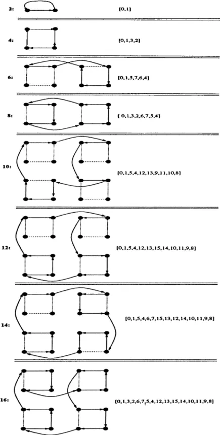
36 3.2 Algorithm for Parallel GSUM O p e r a t io n ...393.3 Communication Protocol for global operations on the hypercube 41 3.4 Ring embedding onto the hypercube ...42
4.1 Algorithm for global shooting patch selection on ring topology . 48 4.2 Example global shooting patch selection on ring topology . . . . 49
4.3 Algorithm for global shooting patch selection on hypercube to p o lo g y ... 50
4.4 Example global shooting patch selection on hypercube topology 54
4.5 Algorithm for Hemicube Production on Ring T o p o lo g y ... 54
4.6 Patch Circulation on a Ring with 4 Processors... 56
4.7 Algorithm for Heniicube Production on Hypercube Topology . . 56
4.8 Patch Circulation on a Three-Dimensional Hypercube ... 57
4.9 Scattered and Tiled D ecom p osition ... 59
4.10 The Form-Factor Vector Circulation Scheme for the Ring Topology 64 4.11 The Contribution Vector Circulation Scheme for the Ring Topol ogy ... 66
4.12 Contribution computation on a Ring with 4 P rocessors... 68
4.13 The Contribution Vector Circulation Scheme for the Hypercube T op ology... 69
4.14 Contribution computation on a Hypercube with 8 Processors . . 70
4.15 Overall efficiency of the Patch Circulation A lg o r it h m ... 76
4.16 Efficiency of the Patch Circulation Scheme per shooting patch . 76 5.1 Abstraction and Representation of the H e m i c u b e ...80
5.2 Algorithm for Form-Factor Vector C o n stru ctio n ... 81
5.3 Algorithm for Hemicube Merging Sch em e... 82
5.4 Ring Algorithm for Naive Hemicube M erging... 85
5.5 Hypercube Algorithm for Naive Hemicube M e r g in g ... 86
5.6 Example execution of
MergeHemicubes2
on a Hypercube with 4 P rocessors... 895.7 Hypercube Algorithm for Communication Efficient Hemicube M e r g in g ... 90
5.8 Subcube Allocation for Hemicube Faces... 95
5.9 Distribution of the Geometry D a t a ... 100
5.10 Mcister-Slave s c h e m e ... 101
5.11 Efficiency of the Hemicube Merging S c h e m e ...102
A .l House Scene Data with 5648 P a t c h e s ...112
A .2 Another view of the house scene d a t a ...113
A .3 A Frame from an animation sequence (3424 p a t c h e s ) ... 113
A .4 Image of a Volkswagen D a t a ... 114
4.1 Effect of local and global shooting patch selection (in Phase 1) on co n v erg en ce... 71
4.2 Effect of the decomposition scheme on the performance of the hemicube production phase (Phase 2) of the parallel algorithm . 73
4.3 Effect of the circulation scheme on the performance of the light contribution computation phase (Phase 4) of the parallel algorithm 74
4.4 Total number of shooting patch selections of the parallel algo rithm normalized with respect to the sequential algorithm . . . 77
5.1 Effect of the Patch Data Decomposition Type on Performance of Hemicube Production Step (Step 2 ) ... 99
5.2 Performance of the proposed parallel hemicube merge algorithm on Hypercube Topology ...100
5.3 Effect of the Hemicube Division Scheme on the Performance of the Parallel S o lu t io n ...103
Chapter 1
Introduction
1.1
Overview
Realistic image synthesis of fictitious environments is one of the major problems of computer graphics, and has a wide range of applications such as animation, C A D , advertising, scientific applications. In order to have photorealistic im age quality, the global illumination of the input environment (indirect lighting, surface-to-surface interreflections and shadows) must be simulated accurately. The original radiosity method is one of the successful solutions to this problem. This method requires excessive time and memory, and the
progressive refine
ment
approach for radiosity has been proposed to provide fast computation rate by approximating the original method. However this method still requires excessive computational power and requires acceleration techniques such as ex ploiting parallelism. This thesis will examine the parallelization of progressive refinement radiosity for medium-to-coarse grain multicomputers.The earlier, but still used, methods for rendering, Gouraud and Phong shading methods [9, 23], assume that objects are illuminated directly by point light sources located at infinity. Although these methods support specular and diffuse illumination; they are local methods, since they ignore the indirect illumination hy surface-to-surface interreflections and shadows caused by occlu sions among the objects. Hence these methods produce incorrect simulations of the light distribution. Ray tracing [44] has become the preferred method for environments consisting of mainly specular surfaces to give solutions that are view-dependent. Hence, the ray tracing method requires recomputation of light distributions each time the viewing position changes. The radiosity
method can successfully compute the ¡nterreflections among diffuse surfaces, which are approximated by a constant “ambient” term in ray tracing. The radiosity method is distinct among the other methods such that it separates the light calculations from the rendering process; once the color (illumination) of each object is calculated, one can walk through the environment without requiring further color calculations.
The
progressive refinement radiosity
method [16] reformulates the original radiosity method and aims to provide approximated solutions initially, in near interactive time. However, the method still requires excessive time in order to provide successful images for complex scenes. Hence, several methods have been proposed in order to speed up the algorithm further. Exploiting paral lelism is among the methods that can achieve good results.1.2
Progressive Refinement Radiosity
The conventional radiosity method is based on radiative heat transfer and was introduced to the field of Computer Graphics by Goral
et al
[22]. The method is based on an energy equilibrium within an enclosure. The objects are given as input with their positions in 3D, their reflectivity and emission values for each colorband. The reflectivity of an object gives the fraction of the incident (impinging) light it disperses and the emission of an object is defined as the amount of light it radiates. The reflectivity and emission values are predetermined which are constants and they depend only on the surface characteristics of the objects. The radiosity method aims to find theradiosity
of each surface element; that is the amount of light energy leaving each surface, which is the sum of emission from the surface and reflection of the incident light (that is the light arriving) at the surface. The incident light is determined by the effects of all other surfaces on the surface, which depends on the geometrical factors as well as the radiosity of other surfaces.'I
The main equation for the radiosity method is:Radiosityi
X Areai
=Emissiorii
x Areai
-|-Reflectancci
x
X
Radiosityj
x Areaj
x F orm Factorsji{l.l)
This equation states that the light leaving from a surface is the sum of light originally emitted from the surface and reflection of the incident light.
CHAPTER 1. INTRODUCTION
The emission (the first term on the right hand side of Eq. 1.1) is equal to 0 if the surface is not a light source. The second term in Eq. 1.1 corresponds to the reflection of incident light. Here,
FormFactorji
denotes the fraction of light energy leaving surfacej
that lands on surface t, to all the energy leaving surfacej.
Note that the radiosity of a surface is dependent on the radiosity of all other surfaces, and Eq. 1.1 holds for each surface; hence combining the equations for all surfaces, a linear system of equations is formed for solving the radiosities of all surfaces, after which the final image can be rendered.The conventional radiosity method, described above, is expensive in terms of execution and the final image cannot be viewed until the matrix equation is solved. This reduces the usability of the method for complex scenes consisting of large number of surfaces, unless the
progressive refinement approach
is used. This new approach eliminates setting up the system of equations, and follows the path the light travels in the environment. The initially approximated solutions are provided quickly and the final solution is approached iteratively. At each iteration:1. The most energetic surface is selected as the source surface, 2. The form-factors from this source surface are computed,
3. Depending on these form-factors, the light is distributed from the source surface to the environment.
In this method, intermediate solutions between the iterations can be viewed, thus allowing the modification of the input scene geometry and surface color properties without waiting until the complete solution is achieved.
1.3 Motivation
Current research in radiosity has concentrated on two main classes: increasing the accuracy and the speed of the solution. The excessive amount of computa tion required by the conventional radiosity led to research for speeding up the solution. Although algorithmic and meshing techniques decrease the execution time, still excessive computational power is required. Hence, exploiting paral lelism can be used for speeding up the method further. However, there is not
much research on parallelization of radiosity. This thesis aims to fill this gap by providing a thorough examination of parallelism in progressive refinement radiosity, and presents two different approaches to parallelization of progressive refinement radiosity on multicomputers. Synchronous parallelism with static task assignment is exploited in order to obtain a solution whose performance does not degrade with simple topologies while exploiting the shooting patch co herence. The two schemes are implemented for ring and hypercube-connected multicomputers on the Intel’s iP S C /2 multicomputer. The performances of the algorithms are analyzed both theoretically and experimentally.
1.4
Outline of the Thesis
This thesis includes three main parts. In the first part, background for the theory of progressive refinement radiosity is provided. The second part dis cusses the design criteria for developing parallel algorithms and previous work on parallelization of the radiosity method. The third part includes two con siderably different approaches for parallel progressive refinement radiosity, the approaches are presented and the theoretical and experimental evaluation of the algorithms are given. Chapter 2 contains the radiosity background. Chap ter 3 contains the parallelization issues for the method. Chapters 4 and 5 present the two novel approaches and give the performance analysis. Chapter 6 includes the concluding remarks, and the discussion of future work directions.
Chapter 2
Radiosity
In this chapter, the realistic image generation problem is stated, the difference between local and global illumination is discussed, and the radiosity method is explained. The chapter continues with the discussion of
progressive refinement
radiosity,
which is investigated for parallelization in this thesis.2.1
Realistic Image Generation
In realistic image generation, the input is a set of objects in 3D with their light characteristics. The output is a photographic quality image of the fictitious scene.
The image synthesis process consists of the following phases:
1. Read in object data from disk.
2. Determine the illumination distribution in the environment and find the color of each object or surface.
3. Render the surface data onto the image and display the image.
The objects are generally approximated by polygons. The input dataset consists of the
(x,y,z)
coordinates and id’s of the polygons in the scene, as well as the reflectivity and the emission of the polygons for color-bands(red,green,blue).
The polygons are assumed to be planar. The final image isa two-dimensional array of pixels for three color-bands. The display of the final image depends on the viewing position and direction of the viewer in three-dimensional coordinates, and the display .process consists of geometrical transformations from the world coordinates to the viewing coordinate system, clipping of the objects to eliminate invisible parts of the objects from the view ing position, and accurate displaying of the objects according to their computed color and geometry.
The method for computing the illumination should be selected carefully in order to get photographical quality images. The illumination models used in this phcise simulate the physical phenomena; and the shadows, which contribute to the quality of the final image are computed.
Earlier, however still in use, illumination methods [9, 23] assume the input objects independently and accept the light sources at infinity in order to com pute the illumination efficiently. In these methods, the color information [23] or the normal vectors [9] are interpolated in order to have smooth shading of the polygons for realistic image generation. However, these methods are
local,
that is they consider only direct illumination from a light source and ignore object-to-object illuminations and shadows caused by occlusions among the objects.Two main global approaches that have been popular and successful at gen erating photographic quality images are
ray tracing
andradiosity.
In ray trac ing, for each pixel on the image plane, a ray is shot and the ray is traversed by reflections and refractions among the objects in the scene. Ray tracing is suitable for scenes consisting of mainly specular surfaces. On the other hand, the radiosity method is successful for environments with diffuse surfaces. The radiosity method is based on an energy equilibrium within a closed environ ment.In ray tracing, the ambient light (i.e. the indirect light resulting from diffuse reflections among the objects) is approximated by a constant factor, however the radiosity method can compute the ambient term more accurately. Another advantage of radiosity over ray tracing is: in an environment with diffuse ob jects, once the light distribution is computed, one can walk through the scene in
near-interactive time with no further light distribution computations, provided that the geometry does not change.
CHAPTER 2. RADIOSITY
seperates the light distribution computation process from the display process. For example, in ray tracing, the light distribution is computed for each im age, as the rays are traversed in the environment. This property makes the radiosity method an efficient method for realistic image synthesis, especially for walkthroughs.
2.2
The Radiosity Method
The radiosity method, based on an energy equilibrium within an enclosure, has its basis in heat transfer between surfaces in an environment [35]. The method was introduced to the field of Computer Graphics by Goral
et al.
[22]. In Computer Graphics, the energy that is transferred is the light energy compared to the heat energy examined by Thermodynamics.The radiosity method assumes perfect Lambertian surfaces (i.e. they emit or reflect light in all directions with equal intensity). Given the objects (sur faces) in the scene with their emissions and reflectivities for three color-bands red, green, blue; the light distribution is formulated based on the surface char acteristics and geometrical relationships. The following equation, which states that light leaving a surface is the sum of self-emitted energy (if the surface belongs to a light-emitter object) and reflection of the incident light incoming from all other surfaces, holds for each surface
i
in the environment:B i
=
E i A i+ r, /
B j F j i d A jJenv j
(
2
.
1
)
where.
R a d io s ity (B ) : The total rate of energy leaving one surface. ( energy/unit area )
E m is s io n (E ) : Rate of energy (light) emitted from a surface. ( energy/unit area )
>
1
R e fle c tiv ity (r ) : Fraction of light reflected back to the environment. ( unitless )
F orm F a cto r(F j,) : Fraction of light leaving surface j which lands on i, to all light leaving j. ( unitless )
A r e a ( A ) : Area of surface ( unit area )
The integral in Equation 2.1 is inefficient to evaluate for differential areas, therefore all the input surfaces in the environment are subdivided into smaller
patches,
which are assumed to have constant radiosity (energy). Then, the following equation holds for each patchi
in the environment:N
BiAi
=EiAi
+ r.BjAjFji, I < i < N
(2.2) J=1R a d io s ity (B ) : The total rate of energy leaving one patch. ( energy/unit time/unit area )
E m issio n (E ) : Rate of energy (light) emitted from a patch. ( energy/unit time/unit area )
R e fle c tiv ity (r ) : Fraction of light reflected back to the environment. ( unitless )
Form F a cto r(F ) : Fraction of light leaving one patch which lands on another. ( unitless )
N : Number of patches in the environment.
Note that the following reciprocity equation holds for each patch pair:
AjF,i
=A,Fij
(2.3)So, Equation 2.2 can be rewritten by using Eq. 2.3 and eliminating A ,’s as:
N
Bi = Ei + r iY B jF ij, l < i < N
j=i(2.4)
Combining Eq. 2.4 for all patches in the environment yields following linear system of equations:
CHAPTER 2. RADIOSITY
-r2F2,\
1 - ^2^2,2-TlFi^N
-‘>’2F2,N
—rjvFTV.l
— V N F N a· · · 1 —
f’f i F N . N Bx ’ Ex ■ B2 = E2 B s En (2.5)Equation 2.5 has to be solved for
B i
’s in three color-bands. The reflectivity r,· and emissionE{
values of the patches are constants and are determined by only the characteristics of the objects which are approximated by patches. In order to solve Eq. 2.5, the form-factor values (F .j’s) should be computed. The form-factor value for a patch depends only on geometrical relationships among the patches and is discussed in the following section.2.2.1
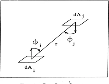
Form-Factor Definition
The form-factor is the fraction of the energy leaving one patch which lands onto another patch, to all the energy leaving the first patch [14, 22, 35]. By definition, the sum of all the form-factors from a patch is equal to unity. The form-factor from a planar or convex patch to itself is zero.
Figure 2.1. Form-Factor Geometry
Figure 2.1 shows the geometric relationships for form-factor computation. In this figure
dAi
anddAj
correspond to differential area elements of patchi
and y, respectively. Then, the form-factor from differential area
i
to differential areaj
is given by:COS^iCOS^j
EdA.dAj = ---J ^ A5
---7Tr
dAidAj
(2,6)
Integrating over patch
j ,
the form-factor from differential areadA{
to areaj
is given as:F
m.
a,
= /COS^iCOS^j
'^^'dAidAj
dAj
(2.7)The form-factor between finite-area patches is defined cis the area average of the differential-to-finite area form-factors:
„ I f f COS^iCOS^i , . , ^
~ ~A J/1, JAi JAja Ja dAjdAi
(
2
.
8
)
Almost always, scenes have occlusions, i.e. some part of the patch is not visible from a second patch because of a third patch between them. Then, a function
SdAidAj
is needed to specify whether the differential areadAi
“sees” differential areadAji
„
I f f COS^iCOS^j
. , A , .^AiAj ~ 'T.
J. J.
SdAidAjdAjdAi
(2.9)/1,
JAi JAj
dAidAj
In Eq. 2.9,
SdAidAj
takes value 1 or 0 depending on the visibility between two differential areasdAj
anddAj.
2.2.2
Form-Factor Computation: Hemicube Method
The hemicube method [14] is proposed in order to provide an efficient, but ap proximated solution to form-factor calculation and it handles occlusions among the patches in the environment. The following subsections discuss the hemicube method in detail.
CUA PTE ft 2. RA DIOSITY
11
Approximations of the Hemicube M ethod
If the distance between two patches is considerably large compared to their size and the effect of occlusion is assumed negligible, the value of the inner integral in Eq. 2.9 remains almost constant because <5,, and r change slightly for differential areas of patch
i
andj.
In this case, the effect of the outer integral is multiplication by unity and the patch-to-patch form-factor is reduced to:A. A,
F,'dAiAj =
I
JA
COS^iCOS^j
TCr
.2dAj
(2
.10
)The source differential area
(dAi)
is selected as the center point of the patchi
in order to represent a well-approximated average position for patchi.
The hemicube method is based on the geometric analogue developed by Nusselt [.35]. The form-factor is equivalent to the fraction of the circle (which is the base of the hemisphere placed over the source patch) that is covered by projecting the destination patch onto the hemisphere and orthographically onto the circle. Figure 2.2 illustrates the geometry of Nusselt’s Analogue. Each point on the circle has an associated delta form-factor, hence the form-factor of a patch is computed by adding the delta form-factors of the points in the projection area.
Figure 2.2. Nusselt’s Analogue
However, discretizing the hemisphere requires creating equal-sized elements on the hemisphere as well as setting up a set of linear coordinates to uniquely
describe locations on the hemisphere surface make the hemisphere method impractical; therefore the hemicube method is used as an approximation of the hemisphere. The hemicube method provides an efficient solution to the form-factor computation for general complex scenes. The method can also be used on special hardware designed for z-buffer hidden surface removal generally used for rendering.
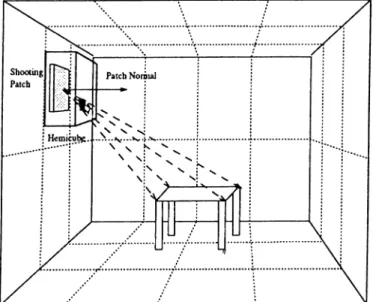
Summary of the Hemicube Method
In the hemicube method, instead of projecting onto a hemisphere, a hemicube is placed onto the center of the source patch (Figure 2..3). Then the environ ment is transformed to the viewing coordinates of the source patch so that the center of the source patch is at the origin and the normal vector of the source patch coincides with the -|-y axis. Hence, five faces of the hemicube (the top face, facing -|-y axis, four side faces facing -x, -fx , -z,
+z
axes) replace the hemisphere. These hemicube faces are divided into small square “pixels” at a given resolution (generally 50x100x100), and the environment is projected and filled onto the five planar faces. If more than one patch project onto the same pixel, the nearest one is selected as the visible patch. This necessitates holding an item-buffer for the hemicube. The item-buffer holds, for each pixel, the id of the patch with nearest distance to the center of the source patch and its distance. This process is similar to thez-buffer
hidden-surface removal [39].CUAFTBfi 2. RADIOSITY
1:3
il.iviiii:, iHojiM'li'd all
I
lie onvironment onto the itein-l)iiir<Ts, IIk' hulh'r en tries are converted to a form-factor vector{Fij,
1 < J <N)
corresponding to the source patchi.
This process consists of adding the delta form-factors of the pixels that correspond to the same patchj
to compute the form-factor valueFij.
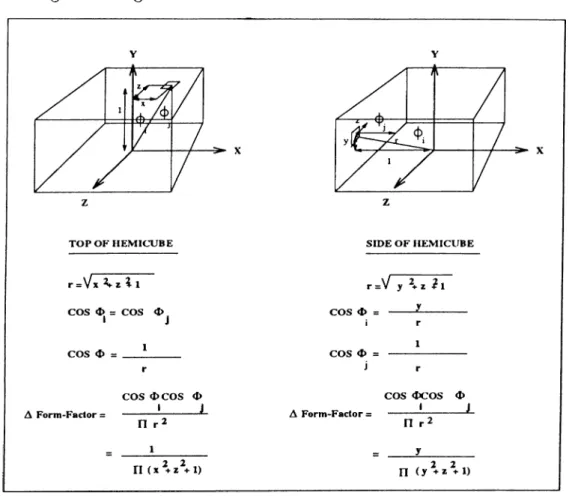
The delta form-factors are computed using the approximation stated in Equation 2.10.The delta form-factor derivation for a pixel on the top face and on a side face are given in Figure 2.4.
Figure 2.4. Delta Form-Factor Derivation
D e ta ile d D e scrip tio n o f the H e m ic u b e M e t h o d
The projection of other patches in the environment onto the hemicube re quires passing all patches through a
projection pipeliiie
consisting ofa)
visibil ity test,b)
clipping,c)
perspective projection, andd)
scan-conversion onto the hemicube faces.a) V isib ility te s t: F’irst, it has to be checked whether the destination patch
j
is potentially visible from the source patch. If patclij
is behind the source patchi
or they do not face each other, then patchj
requires no further computations and leaves the projection pipeline in the early stage.Each planar patch has only one face and a constant normal vector. This normal is computed at the initialization phase of the patch data. Assuming the vertices of the triangular patch are input in clockwise manner, the normal vector of the patch is found as:
N = ( V 3 - V i ) x ( V 2 - V i )
(
2
.
11
)
where and “ x ” are vector subtraction and vector cross product. Figure 2.5 illustrates the geoinetry of the patch normal vector computation.
The visibility test consists of two phases. In the first phase, it is tested whether the two patches face each other. This is accomplished by evaluating the formula:
N j . ( S j - S ¡ ) < 0 (
2.
12)
where N j is the normal vector of patch
j ,
Sj and Sj are the centers of patchi
andj ,
and (Sj — Sj) is the vector connecting the two patch centers which has the starting point at the center point of patchi.
If the dot product “ ·” in Eq. 2.12 is negative, the patch is potentially visible and the visibility test continues. If the dot product is positive, the patches do not face each other and patchj
leaves the projection pipeline.CHAPTER 2. RADIOSITY
15
If the first phase is successful, it is checked whether the destination patch is situated above the source patch plane. This is accomplished by evaluating:
Ni · (V{ - Si) > 0 or Nj · (yj - Si) > 0 or Ni · (V^ - Si) > 0
(2.13)
where ( V j , V2 , V3 ) are the three vertices of the triangular patch
j.
If Equation 2.13 is true, then at least one vertex of the destination patch
j
is above the source patch, so patchj
is potentially visible. Otherwise, patchj
is below the source patch plane, therefore it is not visible, so patchj
leaves the projection pipeline.b ) V ie w in g tra n sfo rm a tio n and clip pin g: The patch that has passed the visibility test is potentially visible. Next, the geometrical transformations have to be performed in order to bring the destination patch
j
to the viewing coordinate system. This is done by setting up the viewing matrix to transform the world coordinated system to the viewing coordinate system for the source patchi
initially and multiplying destination patchesj
in the pipeline with this matrix.When the destination patch
j
has been brought to the viewing coordinate system, it will be projected onto the five faces of the hemicube. If R is the half-width resolution of the hemicube, then a top face with resolution 2Rx2R facing + y direction and four side faces of resolution 2RxR facing -x, + x , -z, + z directions are placed. This results in clipping planesY = X ,Y
=—X, Y =
Z ,Y ^ - Z , Z = - X , Z = X ,Y =
0.When projecting the patch onto a hemicube face, parts of the destination patch
j
which are invisible from patchi
through the hemicube face should be clipped with respect to the surrounding clipping planes of the face. So, the output is a set of vertex points which form the intersection polygon between the input patchj
and the clipping volume defined by four clipping planes. Sutherland-Hodgman [38] polygon clipping algorithm is used in this thesis.c) P e rsp e ctiv e P r o je c tio n : After the destination patch has been clipped with respect to the viewing volume for a hemicube face, only the part of the patch which is inside the volume heis been left. Next, perspective projection with focus length equal to 1 of the vertices is performed to have their coordi nates on the hemicube face.
d )S c a n -co n v e rsio n : Having computed the locations of the vertex ¡)ro- jections on the hemicuhe face, the next process is to “fill” the hemicube face with this patch, considering the hidden surface elimination. First, an edge list corresponding to the points on the edges of the patch is created. Then, the two corresponding edge points for a line are “connected” , interpolating the dis tance. If the pixel buffer has a previous lower distance tlian the patch’s value for that pixel, then there is another patch that is nearer to the source patch for that pixel. Otherwise, the destination patch is nearer, therefore the patch id and distance of that pixel are updated. The similar z-buffer [21] process is exploited in other computer graphics problems such as rendering of the images, in which case the color for that pixel is stored instead of the patch id in the z-buffer.
2.3
Progressive Refinement Radiosity
The conventional radiosity approach has two major disadvantages that limit the usage of the method for complex scenes with large number of patches. First, it requires
O(N^)
time to construct the form-factor matrix (Eq. 2.5){N
is the total number of patches), and the environment cannot be viewed until this operation is completed. Second0{N ^)
memory is needed to store the coefficient matrix. Theprogressive refinement radiosity [\6]
approach provides a solution to these two problems by reformulating the conventional radiosity algorithm. This approach requires0 (N )
time and memory.The progressive refinement approach differs from the conventional radiosity in two aspects. First, the radiosities of all patches are updated simultaneously. Second, the patches are processed in sorted order according to their energy contribution to the environment.
The method starts with an initial approximation to the light distribution in the scene and approaches to more accurate distribution, providing a graceful and continuous convergence to a realistic looking image.
CHAPTER 2. RADIOSIT Y
17
2.3.1
Simultaneous
Update
of Patch
Radiosities:
Shooting vs. Gathering
In the conventional radiosity algorithm, the Gauss-Seidel method is applied to solve the system of equations (Eq. 2.5) for patch radiosities. The method effectively converges to the solution by processing the system of equations one row at a time. The evaluation of the row of the matrix provides an estimate of patch
i
based on the current estimates of the radiosities of all other patches:N
B{
=Ei
+ ?·, ^Bj Fij
, 1 < Î < i=i(2.14)
A single term in Eq. 2.14 gives the light contribution made by patch
j
to patchi:
B{ due to Bj
=I'iBjFij
(2.15)This equation can be reversed by computing the contribution from patch
i
to patchj
using the reciprocity relationship of Eq. 2.3 as follows:Bj due to Bi
=VjBiFji
=VjBiFijAiJAj
(2.16) (2.17)
The contribution to any patch
j
from patchi
is computed using Equa tion 2.17.Note that, the form-factor row corresponding to patch
i
is used to distribute the light energy from patchi
to all other patchesj .
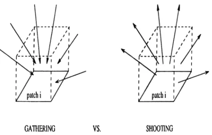
Still, the hemicube method can be used for computing the form-factor row. Thus, each step of the pro gressive refinement radiosity algorithm consists of computing a single row of form-factors for a single patch and adding the light contributions from that patch to all other patches using Eq. 2.17 with computed form-factor values, in effectshooting
the light from that patchi
into the environment.Figure 2.6 illustrates the difference between conventional
[Gathering)
method versus progressive refinement radiosity[Shooting)
method.2.3.2
Solving in Sorted Order
It is desirable for the shooting method to approach to a realistic solution as quickly as possible. At each iteration, the light distribution, that is the radios- ity of each patch
i,
consists of the contributions from the previous shooting patches. The correct distribution is approached faster if the largest contribu tions are added first. Therefore, at each iteration, the patch with maximum energy should be selected for the method to converge faster.Different convergence criterias may be used. In the first criteria, the algo rithm tests the AB,y4, of the shooting patch
i.
If this value is greater than the user-specified tolerance, the algorithm converges. In the second criteria, theABj Aj
values of all the patchesj
in the environment are summed, and tested if this area-weighted sum reaches a specified percentage of the initial energy undistributed in the algorithm.A patch may be selected as the shooting patch more than once during the course of the execution, if it receives more light from the environment. In that case, the environment will already store the estimate of the last shooting from the patch. Hence, a
delta radiosity A B
is stored in addition to the radiosityB
for each patch in order to store the difference between the previous estimate and the current estimate of the patch radiosity, that is the light the patch has gathered since the last shooting from the patch. When solving in sorted order, the solution tends to proceed in approximately the same order as the light propagates through the environment. Figure 2.7 illustrates the pseudo-code for the progressive refinement radiosity algorithm.2.3.3
The Ambient Term
The progressive refinement algorithm starts with a dark environment and grad ually brightens to a globally illuminated scene. In order to view approximately illuminated environments an ambient term is added [16] during the rendering process. The ambient term allows approximate viewing of the initially dark environments. This term decreases as the algoi;^thm converges to more accu rate solutions of
Bj's
with increasing number of shooting patches. Note that, the ambient term is used for display only and is not used in the solution phase.C H A P T E R 2. R A D IO S IT Y
19GATieiNG VS. SHOOTING
Figure 2.6. Shooting versus Gathering (After Cohen
et at)
/ * Initially,
Bi = ABi = Ei
for each patch * / / *Ei
= 0 for non-light sources * /Select patch
i
with greatest A 5 ,A ,. w hile not converged doCalculate form factors at patch i (e.g.using Hemicube Algorithm) for each patch
j
doA Rad = TjABiFijAilAj',
ABj — A B j
-f-ARad",
Bj
=Bj
-fARad;
endforABi =
0Select next patch
i
with greatest A 5 ,A ,. endw hile2.4 Further Improvements of the Method
Although the radiosity method has been successful at generating realistic- looking images, it still has computation and modelling requirements that limit the usage of the method. In this section, a brief overview of these requirements and current research for improving the method will be presented. A summary of previous research on radiosity can be listed as follows:
1. Meshing and preprocessing techniques in order to obtain more accurate and faster solution.
2. Form-factor techniques in order to compute more accurate geometrical relationships among the input patches.
3. Adapting the method for dynamic environments.
4. Including more general reflection models and surface properties such as specularity or participating media in the environment.
5. Exploiting parallelism in order to achieve faster image generation speeds without compromising image quality.
1. M e sh in g and P rep rocessin g T ech n iq u es: The scene models for the radiosity method must satisfy certain constraints in order to obtain an accurate image.
First,
model geometry
requirements state that the input patches have con tinuous normals and homogeneous material properties (such as reflectivity, emission, etc.), the patch dataset is a solid model (the points are classified as inside, on, outside the object), the facets are single sided with consistent normals, and no two faces overlap each other.Second, the
meshing
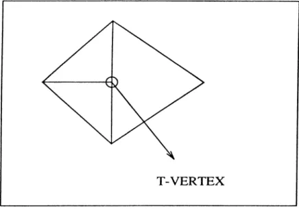
requirements require that no T-vertices occur between neighbouring patches. An example is illustrated in Figure 2.8. Also the poly gons must be well-shaped, that is the ratio of the radius of the inscribed circle to the radius of the circumscribed circle should |)e close to unity, the patches should not be too small or too large, the patches in the environment should be subdivided for better accuracy, and no shadow leakage should occur.Considering these critical issues, several methods have been proposed in order to speed up the solution by using preprocessing techniques for hierarchical
CHAPTER 2. RADIOSITY
21representation of the objects or by starting with coarse patches and adaptively subdividing the necessary regions of the environment during the course of the solution.
Figure 2.8. T-Vertex
The initial work in adaptive subdivision is by Cohen
et al.
[15]. In this work, they propose a subdivision method called “substructuring” with hierarchically subdivision of the input surfaces into subsurfaces, patches and elements. Baumet al.
state the ultimate constraints required by the radiosity method and propose automatic subdivision method [5]. Campbell and Fussell [10] present the subdivision for elimination of light leakage.Hanrahan
et al.
[25] propose a hierarchical representation of the environ ment. In their algorithm, the hierarchical radiosity is inspired by the N-Body problem, and the patch-to-patch visibility is computed and the form-factor computations are performed with required precision. Smitset al
[37] propose a view-dependent solution based on Hanrahan’s work.Lischinski
et al.
[29] propose an accurate radiosity based ondiscontinuity
meshing.
The mesh explicitly represents the discontinuities in the radiance function as boundaries between mesh elements. Piecewise quadratic interpola tion is used to approximate the radiance function. This solution is fully auto matic and view-independent; and is not limited to constant-radiosity patches and produces less number of patch elements.Teller and Sequin [40] propose a visibility prepocessing scheme for inter active walkthroughs in constant environments. The method divides the envi ronment into cells and creates a data structure for cell-to-cell visibility. Then, this data structure is used at the walkthrough stage by computing the cell the viewer is in. So, the potentially visible cell is found and only the patches in this cell are used for rendering the frames.
2. F orm -F a cto r C o m p u ta tio n T ech n iq u es: The hemicube method is an approximation to the hemisphere computation. Although the hemicube method is efficient and it handles occlusions within the environment; it has assumptions which results in incorrect computation of the form-factors.
These assumptions are [3] :
P r o x im ity A s s u m p tio n The hemicube method assumes that the distance between surfaces
i
andj
is great compared to their size, thus the method samples the patchi
with its center point for form-factor computation. This assumption is violated when the two patches are close to each other. V is ib ility A s s u m p tio n The visibility assumption requires that the visibilitybetween differential areas stays constant across patch
i,
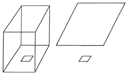
but this assump tion can be violated as shown in Figure 2.9(b). In Fig. 2.9(b), the center of surface 1 has a complete view of surface 2, however shaded part of surface 1 is occluded by surface 3. Thus, the hemicube algorithm will overestimateA lia s in g A s s u m p tio n This assumption states that the surfaces project ex actly onto the hemicube face pixels, similar to the aliasing assumption in rendering and ray tracing. As a result of this assumption, the form-factor value for a surface may be overestimated or underestimated as shown in Figure 2.9(c).
In order to solve the problems caused by the hemicube method assumptions and compute more accurate form-factors, a number of form-factor
computa-'/ ^
tioii techniques have been proposed. Following is a brief summary of these techniques.
The earliest radiosity paper [22] uses direct numerical integration, using Stoke’s Theorem for converting the double integral of the form-factor equation
CHAPTER 2. RADIOSITY
23Figure 2.9. Assumptions of the Hemicube Method (After Baum
et at)
(Eq. 2.8) into a double contour integral. Nishita and Nakamae [i similar solution, by computing the occlusions among the objects.
propose a
In Bu and Deprettere’s approach [7], the form-factor vector is computed by locating a hemisphere over the patch and casting rays towards the hemisphere pixels.
Wallace
et al.
propose [43] a source-to-vertex ray tracing solution. Instead of shooting rays from the source patch in the uniform directions of hemicube pixels, their method samples the shooting patch from the point of view of each other surface in the environment. From each vertex in the environment, rays are sampled towards different parts of the shooting patch, and tested for occlusions by other surfaces.3 . A d a p tin g th e M e t h o d for D y n a m ic E n v iro n m e n ts: The con struction of the form-factor vector is the most compute-intensive part of the radiosity method. When the geometry of the scene changes, these values change and should be re-computed. Some methods have been proposed for providing efficient solutions for dynamic environments.
Baum
et al.
[2]’s method is used for animation. The method computes an animation sequence and the path of the object movement is used for decreasing the form-factor computation time.A ray-tracing based solution [8] was proposed by Buckalew
et al.
in order to be used for incremental updates in geometry and color of the patches.Chen's approach [13] was proposed in order to be used for interactive manip ulation of the objects, based on progressive refinement radiosity. The method works by shooting negative light when a light source is turned off, and com puting the incremental radiosity of the patch when the light attribute of the patch is modified, and computing
incremental form-factor
for a patch when the geometry of the patch changes.4 . In clu d in g M o r e G en era l R eflectan ce M o d e ls : The original ra diosity method assumes ideal Lambertian surfaces, that is the surfaces reflect the incoming light with the same amount in all directions. However, specular reflections and transmissions should be considered for more realistic scenes.
Immel and Cohen [27] propose a method which includes specular reflection. In their approach, a relationship between a given outgoing reflection direction for a patch and all outgoing directions for all other patches is constructed, and a simultaneous solution of the resulting system of equations gives an intensity in each direction for each patch.
Wallace and Cohen [42] propose a two-pass solution. The first pass is view-independent and is based on the hemicube algorithm, with extensions to include the effect of diffuse transmission, and specular-to-diffuse reflection and transmission. The second pass is view-dependent based on distributed ray tracing with z-buffer for specular reflection and transmission.
5. E x p lo itin g P a ra lle lism : Although methods that improve the accu racy and speed of the radiosity method have been presented in the literature, still excessive amount of computation is required to simulate the light dis tribution. Parallelism can be exploited in order to speed up the algorithm further without compromising image quality. In subsequent chapters, the pre vious work on parallelization of the radiosity method is discussed and two novel approaches for parallelization of progressive refinement radiosity will be presented.
CHAPTER 2. RA DIOSITY
252.5
Conclusion and Summary
III this chapter, the global illumination and progressive refinement radiosity is introduced. To summarize, the progressive refinement radiosity algorithm is an iterative approach. Each iteration consists of the following phases:
1. Shooting Patch .Selection.
2. Hemicube Construction for the shooting patch.
3. Conversion of the hemicube item-buifers to a form-factor vector.
4. Contribution computation from the shooting patch to the environment.
In Phase 1, the patch with maximum
ABiA{
is selected as the shooting patch for faster convergence. In Phase 2, all the other patches are projected onto five hemicube faces located on the shooting patch. F’or this process, the patches are passed through a projection pipeline, and the patches which are not visible leave the pipeline in an early stage. In Phase 3, the hemicube is scanned and delta form-factors of the pixels corresponding to the same patch are added in order to obtain the form-factor value for that patch. Phase 4 consists of evaluating Eq. 2.17 for each patchj ,
using the form-factor vector that ha5 been computed for the shooting patch.Overview of Parallelism in Radiosity
This chapter presents the background for the parallel processing and sum marizes the previous efforts for parallelization of the progressive refinement algorithm.
3.1
Classification of Parallel Architectures
In general, parallel architectures can be classified according to:
• the number of instruction and data streams supported, • the memory organization,
• the coupling, • the granularity.
Classification According to the Multiplicity of Data and
Instruction Streams
This classification follows Flynn’s taxonomy [20], and divides the parallel architectures into four classes: '
• S IS D (Single Instruction Single Data) : This is the standard sequential computer.