Outdoor propagation models: applications and considerations for real life problems

Outdoor Propagation Models: Applications and Considerations

for Real Life Problems

Ayhan Altıntaş, Satılmış Topcu, Hayrettin Köymen, Gökhan Moral, Özgür Yılmaz

altintas@ee.bilkent.edu.tr

Abstract: Implementation of propagation prediction models is

discussed. It is shown that for real terrain and building data, the additional parameters and assumptions must be made. The determination of coverage percentages for digital communication is discussed. The results indicate that the field strength predictions depend on the implementation of the model.

Keywords: propagation simulation, coverage, multiple diffraction

loss, outdoor propagation.

Introduction

Propagation prediction lies at the core of the spectrum engineering and management. Signal strength measurements appear to be the natural choice for accurate prediction. In reality, measurements for large-scale point-to-area analyses turn out to be exhaustive, in addition, in today’s overly-crowded spectrum, it may not be possible to do the measurements without any interfering signal. Furthermore, measurements are not suitable to test what-if scenarios. Fortunately, with the advent of computers and availability of high resolution digital terrain data, it is now possible to simulate propagation phenomena within reasonable accuracies. To this end, empirical propagation models are available for a wide range of complexity, accuracy, and input requirements. Some of these models are based on extensive measurement campaigns, such as ITU-R Rec.370 curves [1], some are based on of multiple knife-edge diffraction losses from hilltops or buildings such as Epstein-Peterson [2], Deygout [3], Vogler [4], or Walfish-Ikegami [5]. However, the application of these models presents some details and difficulties for real terrain data. ITU curves do not include the shadowing effects of the hills. ITU recommends clearance angle correction which implicitly takes shadowing into account. But, clearance angle correction is not an adequate description of multiple diffraction loss. Multiple diffraction algorithms are based on idealized conditions and simplifying assumptions. These conditions and assumptions become vague for a real terrain data where identification of separated hills may not be very obvious. There is no clear description of handling these idealized conditions in real problems.

Similar situation exists in urban outdoor wireless propagation models such as Walfish-Ikegami. In this case, propagation is mainly by reflections and diffractions from buildings. Some of the parameters in the model require processing of the input data. So, depending on the input data, an implementation scheme has to be devised.

In this paper, these points will be elaborated and some examples will be provided.

Propagation prediction methods

ITU curves are result of measurement campaigns in the 1950s on different terrain conditions. They predict decreasing field strength with varying attenuation conditions. These conditions are effective transmitting antenna height above average terrain, nature of the terrain (land or sea), statistical time and location percentages,

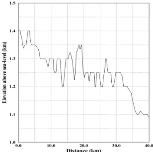
terrain undulation factor (Δh) and height of the receiving antenna. Effective height of the transmitting antenna and Δh are derived from digital terrain elevation data. Usually, terrain elevation data is in the DTED format with 3 arc seconds (Level 1) or 1 arc second (Level 2) resolutions. An example of terrain profile in DTED Level 1 is shown in Figure 1. The profile is away from a transmitter with an effective radiated power of 1kW at f= 30 MHz.

Figure 1. Terrain profile above mean sea-level from TX (N 39º 30’ 30”, E 32º 37’ 45”) in the 180º azimuthally.

ITU curves predict smoothly decreasing field strength away from the transmitter. Therefore strong shadowing right behind the hills is not observed. For this reason, ITU recommends using clearance angle correction to better estimate the field strength behind the hills. A more accurate description of shadowing is given as multiple diffraction loss. ITU-R Recommendation 526 [6] describes Deygout method for multiple diffraction losses.

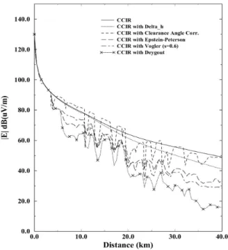
These models have been applied to the terrain profile of Figure 1 and the results are shown in Figure 2. As seen in Figure 2, ITU curves yield generally higher field strength predictions. Although inclusion of Δh correction improves this, it is not to a satisfactory level due to neglect of shadowing in the immediate lee of hilltops. This can partly be accounted for by the inclusion of clearance angle correction. Multiple knife edge diffraction models such as Epstein-Peterson, Deygout or Vogler are intended for better prediction of diffraction loss. The shadowing effect is similarly predicted by all of the diffraction models, but they differ more in the average signal level, as shown in the figure. Note that Epstein-Peterson tends to over-predict while the Vogler method tends to under-predict the average signal level. However, simplicity in applying the Epstein-Peterson method may make it more favourable for some applications.

It is noted that the neither method does not specify how to chose significant knife-edges from the terrain elevation data. To solve this problem, an original selection procedure has been developed that accounts for both the width and the depth of the valleys between local terrain maxima considered as potential knife-edges [7]. Since accounting for too many maxima leads to gross overestimation of the losses, a flexible selection criterion has been introduced. The selection parameter s is the fraction of the Fresnel zone used for making the decision whether two adjacent local maxima should be accounted either as two different knife-edges or as a single dominating knife-edge. The decision is made by the rule that two maxima are distinguished if there is a point in the valley located outside the fraction s of the Fresnel zone connecting the maxima. Alternatively, the maxima are not distinguished if the whole valley is located inside the given fraction of the Fresnel zone. The comparison of the field strength values using different s values is shown in Figure 3. Note that s = 0 is the case when all the local peaks are accounted for as different knife-edges. As seen, this yields lowest values of the field strength. For practical purposes, s = 0.6 seems to be satisfactory.

Figure 2. Comparison of the field strengths predicted by different corrections to ITU curves

As seen from the above discussions, large-scale field strength prediction models may yield substantially different results. The factors affecting the decision of which model to choose depend on the type of landscape, services and frequency band, but may not be totally based on technical concerns. Some government regulatory bodies may prefer to impose one particular model.

Analog Broadcasting and Land Mobile Services

The propagation simulations can be performed with any of the models described in the section above, and the type of simulation can be designed either as a coverage study or interference study. Depending on the type of radio services, the study files generated by simulation of the propagation model are processed to find coverage or interference areas, to calculate link availability, to complete frequency planning and assignment procedures, or to guide international coordination with neighbouring countries. It is generally accepted that coverage contours delimit the field strength levels obtained at about 50 percent of the time. Interference studies are generally based on the possibility of interference at 1 percent of the time. So, time percentages in the ITU curves are recommended

to be taken as 50 percent and 1 percent for coverage and interference studies, respectively. With the aid of a computer software, any coverage or interference contour for a transmitter operating in broadcasting or land mobile service can be displayed on the map. One can directly determine the size of the coverage area or interference area and evaluate other useful data such as the population inside these regions. All these operations require the integration of various databases into the software. In addition, it is deemed to be necessary to integrate the software with a Geographic Information System (GIS) in order to enable display of the simulation results together with the maps and any other spatial data such as roads, boundaries, etc. As an example, Figure 4 shows the coverage area of an analog TV transmitter in Istanbul on the map background. The population covered by this TV station is calculated as 7125501 in a coverage area of 4037 square kilometre. This simulation is carried out by using ITU curves and the effect of terrain is accounted for by using the multiple diffraction technique in which Epstein-Peterson prediction model is exploited.

Figure 3. Comparison of the field strengths predicted by the Vogler method with different s values

Figure 4. Coverage contour (65 dBuV/m) of Çamlıca, İstanbul (N 41º 01’ 40”, E 29º 04’ 08”) analog TV station at UHF IV

band with 37 dBW effective radiated power

In the land mobile service, the coverage and interference areas are evaluated similarly as in the analog broadcasting service except that the receiving antenna height above ground level should be taken as 1.5 or 2 metres in the land mobile, whereas it is taken as

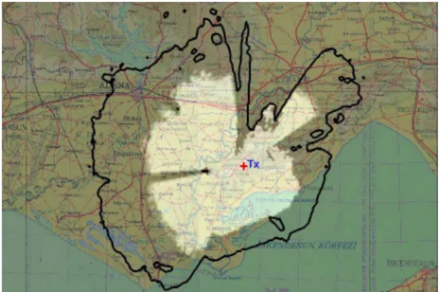
10 metres in analog broadcasting. A study result for a land mobile base station operating at 150 MHz with 25 Watt ERP in Adana is given in Figure 5. The coverage area is surrounded by -90 dBm contour defined by a dark line. Throughout this area, the mobile unit can receive the signals transmitted by the base unit. However, the base unit may not receive the signals coming from the mobile operating with 5 Watt ERP. Therefore, in order to determine a more realistic service area of a land mobile circuit consisting of one base unit and several mobile units, one should evaluate the talk-back range of the mobile. In the talk-back region shown as highlighted in Figure 5, both the base and mobile units can communicate with each other.

Figure 5. Coverage contour (-90 dBm) of Adana (N 36º 49’ 35”, E 35º 37’ 53”) land mobile base station and the talk-back

region of a mobile station in the same circuit

Digital Broadcasting Services

For digital services, the useful (wanted) and interfering (unwanted) signal levels as well as the network gain, protection ratio and coverage probability at all points in the study area must be calculated for a single frequency network (SFN). For a given interference level, the service area where the radio service with sufficient signal quality is provided must be determined. The service area is obtained by finding the regions where the coverage probability is higher than 95 % for DVB and 99 % for DAB.

Coverage probability

The calculation of the coverage probability is split into three parts: calculation of the useful sum field strength, calculation of the interfering sum field strength and evaluation of the coverage probability. For the first two parts, to perform the summation of wanted and unwanted field strengths, several approaches have been reported in the literature [7]. The location variation of field strength is modelled by a log-normal distribution with a standard deviation of 5.5 dB. For determining the power sums of log-normally distributed stochastic variables, we use the k-LNM approach. The k-LNM approach is an approximation method for the statistical computation of the sum of distribution of several log-normally distributed variables [8,9]. The method is based on the assumption that the resulting sum distributions of the wanted and unwanted fields are also log-normal, the mean values and standard deviations of which are taken to be identical with those of the true sum distribution. The k-LNM approach is a modified version of the standard LNM obtained by introducing a correction factor to improve the accuracy in the high probability region. The k-LNM method suffers from the drawback that the correction factor k depends on the number, the powers and the variances of the fields being summed. To obtain optimal results, an interpolation table would be necessary, which is not suitable for an heuristic approach such as k-LNM. For the sake of simplicity, we have chosen an average value of k=0.7 since the standard deviations of the individual fields are small.

Evaluation of the coverage probability is performed by multiplying the probability that the useful sum exceeds a specific value by the probability that the difference between the useful and interfering sums exceeds a specific protection ratio.

To illustrate this methodology, we have performed a case study of single frequency network (SFN) of digital video broadcasting (DVB-T) in Konya lowland of Turkey which has a relatively flat terrain. The SFN consist of six stations located at the corner positions of a hexagon which has edges of 27 km long plus one station at the centre of the hexagon. The station at the centre radiates 100 W and the remaining six stations on the corners of the hexagon cell radiate 1 kW each. The stations are separated by 27 km and their operating frequency is 826 MHz.

Figure 6 shows the useful signal levels and the 48 dB(uV/m) contour that corresponds to the minimum required field strength for the SFN. The locations of the seven DVB transmitters are marked with a plus sign in the plot. In Figure 7, the coverage probability levels with the 95 % coverage probability contour are shown. In addition, the minimum field strength contour is also drawn in Figure 7. It is noted that the 95% coverage probability contour is completely inside the minimum required field strength contour due to the fact that some transmitters behave as interferer in the region surrounded by these two contours.

Figure 6. Useful sum-field strength levels in the service area of a 7-station SFN in DVB-T

Figure 7. The required minimum field strength contour (outer) and 95 % coverage probability contour (inner) on the coverage

Urban Outdoor Cellular Models

The most commonly used empirical model for urban outdoor cellular propagation is Walfish-Ikegami [5] and its extension COST-231 model. The model requires many parameters including, the frequency of operation, the separation between the transmitter and the receiver, the average street width, the average roof height, the receiver antenna height, average building separation, and average orientation angle with respect to the road. In many cases, the building database does not contain any information about the roads, actually, for propagation purposes any separation between the buildings can be treated as roads. So, building data such as in DXF format can be used to derive these parameters. In this format, each building is represented with a polygon with specified height. As an example, a 24 square block building structure (4 by 6) in the form of a Manhattan grid is taken with building height of 10 m. Walfish-Ikegami implementation is compared with ray tracing implementation of a commercial software; the average error between two implementations is shown in Table I for different transmitter height values.

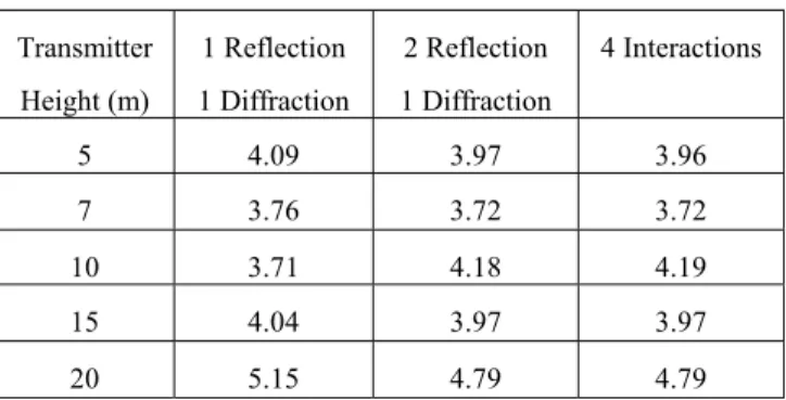
Table 1. The average error between the Walfish-Ikegami and Ray tracing simulation results

Transmitter Height (m) 1 Reflection 1 Diffraction 2 Reflection 1 Diffraction 4 Interactions 5 4.09 3.97 3.96 7 3.76 3.72 3.72 10 3.71 4.18 4.19 15 4.04 3.97 3.97 20 5.15 4.79 4.79 The difference between the Walfish-Ikegami and Ray tracing results show that 4 Interaction result yields similar average errors with 2 reflection and 1 diffraction. In general there is an average error of 3-4 dB levels. Even though this is a significant difference, for the coverage studies it should not be surprising.

Figure 8. Cut off and receiver levels.

Walfish-Ikegami method assumes that the terrain under the buildings is flat. More commonly, the building data is obtained from aerial or satellite 3-D imagery which includes the warping of

the terrain profile. So, a cut-off level has to be chosen to take a reference flat earth under the buildings as shown in Figure 8. If this level is chosen too high, then some receiver points will be under ground level, resulting wrong signal levels. If the level is chosen too low, then the receiver height may become too high to be used in the method. For these reasons, we recommend choosing the cut-off reference level for each receiver point separately.

Conclusions

Different propagation prediction models are discussed. Their implementation on real terrain and building data is discussed. It is seen that, on real terrain some additional assumptions and parameters should be taken into account. These parameters and assumptions may yield different field strength predictions. These parameters are identified for large-scale models and urban models for cellular communications.

References

[1] ITU-R Recommendation P.370-7, “VHF and UHF Propagation Curves for the Frequency Range from 30 MHz to 1000 MHz’’, Geneva, 1995.

[2] Epstein, J. and Peterson, D.W., “An Experimental Study of Wave Propagation at 850 MC’’, Proceedings of Institute of Radio Engineering, 41, pp.595-611, 1955.

[3] Deygout, J., “Correction Factor for Multiple Knife-edge Diffraction’’, IEEE Trans. on Antennas and Propagation, AP-39, pp.1256-1258, 1991.

[4] Vogler, L.E., “An Attenuation Function for Multiple Knife-edge Diffraction’’, Radio Science, 17, pp.1541-1546, 1982. [5] J. Walfisch and H.L. Bertoni, “A Theoretical Model of UHF Propagation in Urban Environments’’, IEEE Trans. on Antennas and Propagation, AP-36, no.12, pp.1788-1796, Dec. 1988.

[6] ITU-R Recommendation P.526-5, “Propagation by Diffraction’’, Geneva, 1997.

[7] S. Topcu, H. Koymen, A. Altintas, and I. Aksun, “Propagation Prediction and Planning Tools for Digital and Analog Terrestrial Broadcasting and Land Mobile Services’’, Proc. of 50th Annual Broadcast Symposium, Virginia, USA, Sept. 2000. [8] Beaulieu, N.C., Abu-Dayya, A.A., and MvLane, P.J., “Estimating the Distribution of a Sum of Independent Log-normal Random Variables’’, IEEE Trans. on Communications, 43 (12), pp.2869-2873, 1995.

[9] European Broadcasting Union, “Technical Bases for T-DAB Services Network Planning and Compatibility with Existing Broadcasting Services’’, EBU Document, BPN003, Rev.1, May 1998.

[10] European Broadcasting Union, “Terrestrial Digital Television Planning and Implementation Considerations’’, EBU Document, BPN005, Second Issue, July 1997.