Dynamical analysis of a discrete conformable fractional order bacteria population model in a microcosm

Contents lists available atScienceDirect

Physica A

journal homepage:www.elsevier.com/locate/physa

Dynamical analysis of a discrete conformable fractional order

bacteria population model in a microcosm

Guven Kaya

a

_{, Senol Kartal}

b,∗

, Fuat Gurcan

c

a_{Department of Mathematics, Faculty of Arts and Sciences, Bingol University, Bingol, 12000, Turkey}

b_{Department of Science and Mathematics Education, Nevsehir Haci Bektas Veli University, Nevsehir 50300, Turkey} c_{Department of Mathematics, Faculty of Science, Kuwait University, Safat, 13060, Kuwait}

a r t i c l e i n f o

Article history:

Received 16 May 2019

Received in revised form 21 November 2019 Available online 17 December 2019

Keywords:

Conformable fractional derivative Piecewise constant arguments Stability

Flip and Neimark–Sacker bifurcation

a b s t r a c t

In this paper, conformable fractional order differential equations with piecewise con-stant arguments are used for a modeling population density of a bacteria species in a microcosm. The discretization process of a differential equation with piecewise constant arguments gives us two dimensional discrete dynamical system in the interval t ∈ [nh,(n+1)h). By using the center manifold theorem and the bifurcation theory, it is shown that the discrete dynamical system undergoes flip and Neimark–Sacker bifurcation depending on the parameter r. It is observed that the model describes some biological phenomena for a bacteria population such as homogeneous bacteria distributions and inhomogeneous spatial population distributions. In addition, the effect of fractional order derivative on dynamic behavior of the system is investigated. Finally, all theoretical results are supported by numerical simulations.

© 2019 Elsevier B.V. All rights reserved.

1. Introduction

Micro- and mesocosms are experimental ecosystems of any habitat type, which contain more than one species that can investigate various ecological endpoints. They provide a bridge between laboratory and field studies, preserving some of the natural conversion of field studies, with a greater control of conditions and changeables, as well as reproduction, and are therefore an extremely useful tool to investigate how ecosystems answer to stress. Therefore microcosms have been used as tools [1–7] for studying population dynamics such as bacteria growth. In study [5], Gause created a microcosm of a nutritive decoction of bacteria and studied the variations in the populations over a few days. It is observed that experimental and theoretical results are consistent with each other. Grigoryan et al. [6] have examined the diversity and sulfide-producing activity of microorganisms in microcosms containing commercial clay products. In study [7], Multi-species microcosms have been used to investigate effects of ionizing radiation in a model freshwater ecosystem, including endpoints at both structural and functional levels and ecological interactions. In study [8], substrate supplied to the microhabitats facilitates bacterial growth, and microbial cells can migrate between neighboring microhabitats due to random motility, chemotaxis towards substrate and self-attraction.

The mathematical approximation for population growth in some biological situations includes nonlinear differential equations. It is generally known that a differential equation model is preferred for the overlapping generation of a single species [9,10]. If there is only single species that does not overlap, then it is appropriate to build a model with the difference equation [11]. In recent years, there is a significant increase in the use of fractional-order derivatives into

∗

Corresponding author.

E-mail addresses: gkaya@bingol.edu.tr(G. Kaya),senol.kartal@nevsehir.edu.tr(S. Kartal),fgurcan@sci.kuniv.edu.kw(F. Gurcan). https://doi.org/10.1016/j.physa.2019.123864

many disciplines such as mechanics, chemistry, biology, mathematics and physics [12–15]. The fractional derivative gives an excellent instrument for the description of memory and hereditary properties of various materials and processes. It has been exposed that, the fractional derivative is more suitable for modeling real world problem than ordinary derivative of integer order [16–20].

There are many definitions of the fractional derivative and the most common known are Riemann–Liouville and Caputo derivative. However, Caputo and Riemann–Liouville also have a big problem that, their kernel although nonlocal but is singular. This weakness has effect when modeling real world problem [21]. Therefore, some researchers have introduced the concept of non-local derivative. In [22], Khalil presented a new definition of derivative prominently compatible with the classical derivative. This operator is called conformable derivative and satisfy some conventional properties such as chain rule and have properties similar to the ordinary Newton’s calculus. Moreover, biological and physical applications of conformable fractional derivative can be found in [23–25]. According to this definition, the left conformable fractional derivative starting from a of the function f

: [

a

, ∞

)

→ ∞

of order 0

< α ≤

1 is defined by

(T_αaf )(t)

=

lim

ϵ→0

f (t

+

ϵ

(t

−

a)1−α

)

−

f (t)

ϵ

(1)

and the right conformable fractional derivative of order 0

< α ≤

1 terminating at b of f is defined by (b_αTf )(t)

= −

lim

ϵ→0

f (t

+

ϵ

(b

−

t)1−α

)

−

f (t)

ϵ

.

(2)

Note that if f is differentiable then

(T_αaf )(t)

=

(t

−

a)1−αf′(t)

,

(b_αTf )(t)

= −

(b

−

t)1−αf′(t)

.

(3) In dynamical system, bifurcation and chaos have become an important topic and appear naturally in several important biological models [10,26–31]. In study [10], May has already pointed out that a simple deterministic model can exhibit chaotic behaviors, and the importance of chaos in ecology. Chaotic behavior can be observed as a result of flip and hopf bifurcation that occur with the presence of periodic or quasi-periodic solutions and in this case the dynamic behavior of the system is very sensitive to the initial conditions. As a generalization of the integer-order systems, the fractional-order nonlinear dynamic systems display numerous dynamic behaviors as in integer-fractional-order systems, such as attractor, bifurcation, and chaos. Studies have shown that fractional order nonlinear systems exhibit more complex dynamic behavior then the integer-order systems because of its memory effect. Therefore, the study of fractional chaotic systems has become increasingly interesting and numerous fractional nonlinear systems with chaotic behaviors have been found in [32–35].

Another approach taken into account in modeling biological systems is using differential equations with piecewise constant arguments. These equations describe hybrid dynamical systems and combine properties of both differential and difference equations and have applications in widely expanded areas such as biomedicine, chemistry, mechanical engineering, physics and population dynamics [26,27]. Ozturk et al. [4] modeled a population density of a bacteria population in a microcosm such as

dx(t)

dt

=

rx(t)(1

−

α

x(t)

−

β

0x(

[

t

]

)

−

β

1x(

[

t

−

1

]

)) (4)

where t

≥

0 and

[

t

]

denotes the integer part of t

∈ [

0

, ∞

). x(t) represent green algae (Chlorella) and rotifers (Lepadella) bacteria population in a subculture solution (10 ml) and the initial value of the bacteria population density is nearly 104_(cells

_/

_{ml) and the equilibrium point is approximatelyx}

_¯

₌

₅

_×

₁₀5_{and also the upper bound of the bacteria population}

density is 7

×

107_{. The parameter r is the population growth rate of the bacteria population,}

_α

_,

_β

0and

β

1are coefficients

that each represents the irregular environmental carrying capacity for a logistic population model.

The aim of this study is to investigate dynamical behavior of conformable fractional order form of the model(4)that is given as follows; Tqx(t)

=

rx(t)(1

−

α

x(t)

−

β

0x(

[

t h

]

h)

−

β

1x(

[

t

−

h h

]

h))

.

(5)

where

[

t

]

denotes the integer part of t

∈ [

0

, ∞

) and h is discretization parameter.

In the literature, there are limited numbers of studies about modeling population dynamics by using conformable fractional order differential equations [23–25]. In our study, we use conformable fractional order which capture local memory effect for a population but this event cannot be reflected with ordinary differential equations. Biologically, memory effect means that the growth rates of populations not only depend on the current conditions, but also depend on all previous conditions. In view of this, model(5)is a more realistic than the model(4)formed by integer-order differential equations. In addition, we also deal with relatively new discretization process based on the piecewise constant functions for conformable fractional order differential equations [25]. The use of piecewise constant functions allows us to convert differential equation(5)to difference equations. Hence, flip bifurcation, Neimark–Sacker bifurcation and chaotic dynamics for a bacteria population will be easily examined through this discrete system.

2. Discretization process

In this section, we will discretize the model(5) based on approximation given in [25]. From the left conformable fractional derivative, we get

(t

−

nh)1−qdx(t) dt

=

rx(t)(1

−

α

x(t)

−

β

0x(

[

nh h

]

h)

−

β

1x(

[

nh

−

h h

]

h))

.

(6)

We can rewrite Eq.(6)as following form,

−

x ′ (t) x2_(t)

−

r

β

0x(nh)

+

r

β

1x(nh

−

h)

−

r (t

−

nh)1−q 1 x(t)

=

α

r (t

−

nh)1−q

.

(7)

Solving this equation with respect to t

∈ [

nh

,

t), we obtain

x(t)

=

(1

−

β

0x(nh)

−

β

1x((n

−

1)h))x(nh)

(1

−

β

₀x(nh)

−

β

₁x((n

−

1)h)

−

α

x(nh))e−r(1−β0x(nh)−β1x((n−1)h))(t−nh)q_q

₊

_α

x(nh)

.

(8)

Let t

→

(n

+

1)h, then we have the following difference equation

x((n

+

1)h)

=

(1

−

β

0x(nh)

−

β

1x((n

−

1)h))x(nh)

(1

−

β

₀x(nh)

−

β

₁x((n

−

1)h)

−

α

x(nh))e−r(1−β0x(nh)−β1x((n−1)h))hqq

₊

α

_x(nh)

.

(9)

Finally, adjusting difference equation notation and replacing x(nh) and x((n

−

1)h) by x(n) and x(n

−

1) yields

x(n

+

1)

=

(1

−

β

0x(n)

−

β

1x(n

−

1))x(n)

(1

−

β

₀x(n)

−

β

₁x(n

−

1)

−

α

x(n))e−r(1−β0x(n)−β1x(n−1))hqq

₊

α

_x(n)

(10)

If we change of variables to u1(n)

=

x(n) and u2(n)

=

x(n

−

1), we get the two-dimensional discrete system as follows:

⎧

⎨

⎩

u1(n

+

1)

=

(1

−

β

₀u1(n)

−

β

1u2(n))u1(n) (1

−

α

u1(n)

−

β

0u1(n)

−

β

1u2(n))e −r(1−_β0u1(n)−β1u2(n))hqq

₊

α

_u 1(n) u2(n

+

1)

=

u1(n)

.

(11) 3. Stability analysis

Direct calculations show that the system(11)has a positive equilibrium point E∗

₌

(u∗ 1

,

u ∗ 2)

=

( 1 α+β0+β1

,

1 α+β0+β1) and

corresponding Jacobian matrix at this equilibrium point is

J(E∗)

=

⎛

⎜

⎝

e −_αrhq (α+β0+β1 )q₍

α + β

₀₎

−

β

₀

α

βα1(

−

1

+

e −_αrhq (α+β0+β1 )q₎ 1 0

⎞

⎟

⎠ .

Moreover, the characteristic polynomial of J(E∗

) is given by: p(

λ

)

=

λ

2

+

(

β

0

α

−

e −_(α+βαrhq 0+β_{1 )q(1}

₊

β

0

α

))

λ −

β

1

α

(e −_(α+βαrhq 0+β_{1 )q}

₋

₁₎

.

₍₁₂₎

The following theorem confirms the stability of positive equilibrium point of the model(11)under some conditions.

Theorem 1. Let

β

₀

> α + β

₁

>

2

α

. The following statements are true.

(i) Suppose that 3

β

1

< α + β

0. The positive equilibrium point of system(11)is local asymptotically stable if and only if

0

<

r

<

q(

α + β

0

+

β

1)

α

hq ln(

α + β

0

−

β

1

β

0

−

α − β

1

)

.

(13)

(ii) Suppose that 3

β

1

> α + β

0. The positive equilibrium point of system(11)is local asymptotically stable if and only if

0

<

r

<

q(

α + β

0

+

β

1)

α

hq ln(

β

1

β

1

−

α

)

.

(14)

Proof. By the Linearized Stability Theorem in [36] we get that the positive equilibrium point of the system(11)is locally asymptotically stable if and only if

⏐

⏐

⏐

⏐

β

0

α

−

e − αrhq (α+β0+β1 )q₍₁

+

β

0

α

)

⏐

⏐

⏐

⏐

<

1

−

β

1

α

(

e− α rhq (α+β0+β1 )q

−

1

)

<

2

.

(15)

(a)

⏐

⏐

⏐

⏐

β

0

α

−

e − αrhq (α+β0+β_{1 )q(1}

₊

β0 α)

⏐

⏐

⏐

⏐

<

1

−

β1 α

(

e− α r α+β0+β₁

₋

₁

)

(b) 1

−

β1 α

(

e− α rhq (α+β0+β1 )q

−

1

)

<

2. From (a), we will get

r

<

q(

α + β

0

+

β

1)

α

hq ln(

α + β

0

−

β

1

β

0

−

α − β

1

) (16)

where

β

0

> β

1

+

α

. Furthermore, from (b), we obtain

r

<

q(

α + β

0

+

β

1)

α

hq ln(

β

1

β

1

−

α

) (17)

where

β

1

> α

. Considering(16)and(17)with the fact that for 3

β

1

< α + β

0we hold

0

<

r

<

q(

α + β

0

+

β

1)

α

hq ln(

α + β

0

−

β

1

β

0

−

α − β

1 )

<

q(

α + β

0

+

β

1)

α

hq ln(

β

1

β

1

−

α

) and for 3

β

1

> α + β

0one can obtain

0

<

r

<

q(

α + β

0

+

β

1)

α

hq ln(

β

1

β

1

−

α

)

<

q(

α + β

0

+

β

1)

α

hq ln(

α + β

0

−

β

1

β

0

−

α − β

1 ) This completes our proof.

4. Bifurcation analysis

Bifurcation analysis is a very important issue for a better understanding mechanism of the biological models in both discrete and continuous time dynamical systems. In this section, we choose the parameter r as a bifurcation parameter for analyzing the Flip and Neimark–Sacker bifurcation of the system(11)at the equilibrium point E∗

by using the center manifold and bifurcation theory in [28–31,37,38]

4.1. Flip bifurcation analysis

In this section, we discuss the existence and direction of flip bifurcation for the system.

Theorem 2. Suppose that the parameters satisfy

β

0

> α + β

1

>

2

α

and 3

β

1

< α + β

0. If

α

1

̸=

0,

α

2

̸=

0 and

r1

=

r1∗

=

q(

α + β

0

+

β

1)

α

hq ln(

α+β0−β1

β0−α−β1) then the system(11) undergoes Flip bifurcation at the equilibrium point (u ∗

1

,

u

∗

2).

Moreover, if

α

2

>

0 then the period-2 solution is stable, and if

α

2

<

0 then the period-2 solution is unstable. Proof. If r∗

1

=

q(

α + β

0

+

β

1)

α

hq ln(

α+β0−β1

β0−α−β1), then the eigenvalues of Jacobian matrix at equilibrium point (u ∗ 1

,

u ∗ 2) are

λ

1

= −

1 and

λ

2

=

2

β

1

β

1

−

a

−

β

0

. The condition

|

λ

₁

| ̸=

1 leads to

α + β

0

̸=

3

β

1.

To decide the stability of the bifurcated period-2 points, we apply the center manifold reduction. Takingr as an

¯

independent variable into the system(11)and making transformation: u

=

u1

−

u∗1,

v =

u2

−

u∗2ve

¯

r

=

r

−

r

∗

1, then the

system(11)is transformed into:

(

_u

¯

r

v

)

→

⎛

⎜

⎝

α + β

0

+

β

1

β

1

−

β

0

−

α

0 2

β

1

β

1

−

β

0

−

α

0 1 0 1 0 0

⎞

⎟

⎠

(

_u

¯

r

v

)

+

(

_{f (u}

, ¯

_r

, v

₎ 0 0

)

(18) where f1(u

, ¯

r

, v

)

=

m13u2

+

m14r

¯

2

+

m15

v

2

+

m16u

¯

r

+

m17u

v +

m18r

¯

v +

o

(

(|

u

| + |

r

| + |

v|)

3

)

and the Taylor coefficients mijare

m13

=

(

α + β

0)(

α − β

0

+

β

1)(

α + β

0

+

β

1)((

α + β

0)(2

α −

ln(β1 −β₀−α α−β0+β1)

β

0)

+

ln( β1−β0−α α−β0+β1)

β

0

β

1)

α

2₍

_{α + β}

0

−

β

1)2

,

m14

=

0

,

m15

=

(ln(β1−β0−α α−β0+β1)

+

2

α

β

1

−

β

0

−

α

)(

α − β

0

+

β

1)(

α + β

0

+

β

1)

β

12

α

2₍

β

1

−

β

0

−

α

)

,

m16

=

hq₍

_{α + β}

0)(

α − β

0

+

β

1) q(

α

2

₊

₂

αβ

0

+

β

02

−

β

12)

,

m17

=

β

1(

α − β

0

+

β

1)(

α + β

0

+

β

1)

α

2₍

α + β

0

−

β

1)2

×

((

α + β

0)(

α

(4

−

ln(

β

1

−

β

0

−

α

α − β

0

+

β

1 ))

+

2ln(

β

1

−

β

0

−

α

α − β

0

+

β

1 )

β

0)

+

ln(

β

1

−

β

0

−

α

α − β

0

+

β

1 )(

α +

2

β

0)

β

1) m18

=

hq

_β

1(

α − β

0

+

β

1) q((

α + β

0)2

−

β

12)

.

Let T

=

⎛

⎜

⎝

1 0 2

β

1

β

1

−

β

0

−

α

0 1 0 1 0 1

⎞

⎟

⎠

and use the translation

(

_u

¯

r

v

)

=

T

(

_X

µ

Y

)

. Then the map(18)becomes

(

_X

µ

Y

)

→

⎛

⎜

⎝

−

1 0 0 0 1 0 0 0 2

β

1

β

1

−

β

0

−

α

⎞

⎟

⎠

(

_X

µ

Y

)

+

(

_F 1(X

, µ,

Y ) 0 F2(X

, µ,

Y )

)

,

(19) where F1(X

, µ,

Y )

= −

(m13

+

m16)(

α + β

0

−

β

1)

α + β

0

−

3

β

1

µ

2

−

(m13

+

m15

−

m17)(

α + β

0

−

β

1)

α + β

0

−

3

β

1 X2

+

(2m13

+

m16

−

m17

−

m18)(

α + β

0

−

β

1)

α + β

0

−

3

β

1 X

µ

−

(m17

+

m18)(

α + β

0

−

β

1)

−

2(2m13

+

m16)

β

1 (

α + β

0

−

3

β

1)(

α + β

0

−

β

1) Y

µ

−

m15(

α + β

0

−

β

1) 2

₊

₂

_β

1(

−

m17(

α + β

0

−

β

1))

+

2m13

β

1 (

α + β

0

−

3

β

1)(

α + β

0

−

β

1)2 Y2

−

2m15(

α + β

0

−

β

1)

+

4m13

β

1

−

m17(

α + β

0

+

β

1)

α + β

0

−

3

β

1 XY and F2(X

, µ,

Y )

=

(m13

+

m16)(

α + β

0

−

β

1)

α + β

0

−

3

β

1

µ

2

+

(m13

+

m15

−

m17)(

α + β

0

−

β

1)

α + β

0

−

3

β

1 X2

−

(2m13

+

m16

−

m17

−

m18)(

α + β

0

−

β

1)

α + β

0

−

3

β

1 X

µ

+

(m17

+

m18)(

α + β

0

−

β

1)

−

2(m13

+

m16)

β

1

α + β

0

−

3

β

1 Y

µ

+

2m15(

α + β

0

−

β

1)

+

4m13

β

1

−

m17(

α + β

0

+

β

1)

α + β

0

−

3

β

1 XY

+

m15(

α + β

0

−

β

1) 2

₋

₂

_β

1(m17(

α + β

0

−

β

1)

−

2m13

β

1) (

α + β

0

−

3

β

1)(

α + β

0

−

β

1) Y2

.

Suppose that Wc(0)

= {

(X

, µ,

Y )

∈

R3

|

Y

=

h∗(X

, µ

)

,

h∗(0

,

0)

=

0

,

Dh∗(0

,

0)

=

0

}

is the center manifold for the system of (X

,

Y )

=

(0

,

0) near

µ =

0. Assume that

By approximate computation for the center manifold, we have A

=

(m13

+

m15

−

m17)(

α + β

0

−

β

1) 2 (

α + β

0

−

3

β

1)(

α + β

0

+

β

1) B

=

(2m13

+

m16

−

m17

−

m18)(

α + β

0

−

β

1) 2 (

α + β

0

−

3

β

1)2 G

=

(m13

+

m16)(

α + β

0

−

β

1) 2 (

α + β

0

−

3

β

1)(

α + β

0

+

β

1)

Now, the map(19)restricted to the center manifold is given by

˜

F

:

X

→ −

X

+

h1X2

+

h2X

µ +

h3

µ

2

+

h4X3

+

h5X2

µ +

h6X

µ

2

+

h7

µ

3

+

O((

|

X

| + |

µ|

)4) (20) where h1

= −

(m13

+

m15

−

m17)(

α + β

0

−

β

1)

α + β

0

−

3

β

1 h2

=

(2m13

+

m16

−

m17

−

m18)(

α + β

0

−

β

1)

α + β

0

−

3

β

1 h3

= −

(m13

+

m16)(

α + β

0

−

β

1)

α + β

0

−

3

β

1 h4

= −

(m13

+

m15

−

m17)(

α + β

0

−

β

1)2(2m15(

α + β

0

−

β

1)

+

4m13

β

1

−

m17(

α + β

0

+

β

1)) (

α + β

0

−

3

β

1)2(

α + β

0

+

β

1) h5

=

(

α + β

0

−

β

1)2 (

α + β

0

−

3

β

1)3(

α + β

0

+

β

1)

[−

(

−

m16m17

+

m15(2m16

−

m17

−

m18)

+

m13(4m15

−

m17

+

m18))(

α + β

0)2

−

2(2m213

+

3m17(m17

+

m18)

+

m13(

−

2m15

+

m16

−

4(m17

+

m18))

−

m15(m16

+

2(m17

+

m18)))(

α + β

0)

β

1

+

(

−

20m213

+

m13(

−

8m15

−

10m16

+

15m17

+

m18)

+

m17(7m16

+

2(m17

+

m18))

−

m15(4m16

+

5(m17

+

m18)))

β

12

]

h6

= −

(

α + β

0

−

β

1)2 (

α + β

0

−

3

β

1)3(

α + β

0

+

β

1)

[

(2m15m16

+

m16m18

−

(m17

+

m18)2)(

α + β

0)2

−

2m16(4m15

+

m16

−

2m17

−

m18)(

α + β

0)

β

1

+

(6m15m16

−

2m162

+

(m17

+

m18)2

+

m16(4m17

+

m18))

β

12

−

4m213

β

1(

α + β

0

+

5

β

1)

+

m13((2m15

+

m17

+

2m18)(

α + β

0)2

−

2(4m15

+

2m16

−

3m17

−

2m18)(

α + β

0)

β

1

+

(6m15

−

20m16

+

5m17

+

2m18)

β

12)

]

h7

=

(m13

+

m16)(

α + β

0

−

β

1)2(

−

(m17

+

m18)(

α + β

0

−

β

1)

+

2(2m13

+

m16)

β

1) (

α + β

0

−

3

β

1)2(

α + β

0

+

β

1)

.

As given by the flip bifurcation theorem in [39], the emergence of flip bifurcation for map(20)requires

α

1

=

[

∂

F

∂µ

.

∂

2_F

∂

X2

+

2

∂

2_F

∂

X

∂µ

] ⏐

⏐

⏐

⏐

(0,0)

=

2(2m13

+

m16

−

m17

−

m18)(

α + β

0

−

β

1)

α + β

0

−

3

β

1

̸=

0 and

α

2

=

[

1 2

.

(

∂

2_F

∂

X2

)

2

+

1 3

.

∂

3_F

∂

X3

]

⏐

⏐

⏐

⏐

(0,0)

=

2(m13

−

m15)(m13

+

m15

−

m17)(

α + β

0

−

β

1) 2 (

α + β

0

−

3

β

1)(

α + β

0

+

β

1)

̸=

0

.

Thus, the proof is completed.

4.2. Neimark–Sacker bifurcation analysis

As stated by the Neimark–Sacker bifurcation theorem in [39], the existence of the Neimark–Sacker bifurcation for the system requires some conditions that are eigenvalue assignment, transversality and nonresonance conditions. The following theorem is obtained for analyzing these conditions and it also give the direction of Neimark–Sacker bifurcation.

Theorem 3. Assume that the parameters satisfy

β

0

> α + β

1

>

2

α

and 3

β

1

> α + β

0. If

β

1

̸=

α + β

0, 2

β

1

̸=

α + β

0, k

̸=

0

and r

=

r∗

2

=

q(

α + β

0

+

β

1)

α

hq ln(

β1

β1−α) then the system(11)undergoes Neimark–Sacker bifurcation at the equilibrium point

(u∗

1

,

u

∗

2). In addition to, if k

<

0 then an attracting invariant cycle will appear for r

>

r

∗

2, if k

>

0 then a repelling invariant

cycle will appear for 0

<

r

<

r∗

Proof. Suppose that r∗

2

=

q(

α + β

0

+

β

1)

α

hq ln(

β1

β1−α). The characteristic equation of the model(11)at the equilibrium point

(u1(r2∗)

,

u2(r2∗)) is obtained by

λ

2

₊

α + β

0

−

β

1

β

1

λ +

1

=

0

.

(21)

The eigenvalues of Eq.(21)are

λ

1,2(r ∗ 2)

=

β

1

−

β

0

−

α

2

β

1

±

i

√

(

α + β

0

−

3

β

1)(

α + β

0

+

β

1) 2

β

1

=

a

±

ib

.

We get

⏐

⏐

λ

₁,₂(r₂∗)

⏐

⏐ =

1 and the transversality condition gives to the inequality

d

⏐

⏐

λ

₁,₂(r)

⏐

⏐

dr

⏐

⏐

⏐

⏐

r=r₂∗

= −

h q₍

_{α − β}

1)(

α

2

+

β

02

+

β

0(2

α − β

1)

−

αβ

1

−

β

21) q

β

1(

α + β

0

+

β

1)

√

2(

α

2

₊

_β

2 0

+

2

β

0(

α − β

1)

−

2

αβ

1

−

β

12)

̸=

0

.

Moreover, if

β

1

̸=

α + β

0and 2

β

1

̸=

α + β

0then we have

λ

n1,2(r

∗

2)

̸=

1 (n

=

1

,

2

,

3

,

4).

Let u

=

u1

−

u∗1and

v =

u2

−

u∗2, then the system(11)is transformed into

(

u

v

)

→

(

β

₁

−

β

₀

−

α

β

1

−

1 1 0

)

(

u

v

)

+

(

f (u

, v

) 0

)

(22) where f (u

, v

)

=

s13u2

+

s14u

v +

s15

v

2

+

s16u3

+

s17u2

v +

s18u

v

2

+

s19

v

3

+

o

(

(|

u

| + |

v|)

4

)

(23)

and the Taylor coefficients sijare

s13

=

(

α + β

0)(

α − β

1)(

α + β

0

+

β

1)(

α

2

+

β

0(

α −

ln(_β1β−1_α)

β

1))

α

2

β

2 1

,

s14

=

(

α − β

1)(

α + β

0

+

β

1)(2

α

(

α + β

0)

−

ln(_β1β−1α)(

α +

2

β

0)

β

1)

α

2

_β

1

,

s15

=

(

α − β

1)(

α + β

0

+

β

1)(

α −

ln(_β1β−1α)

β

1)

α

2

,

s16

=

(

α + β

0)(

β

1

−

α

)(

α + β

0

+

β

1)2 2

α

3

β

3 1

×

[

2

α

2(

α + β

0)2

−

2

α

(1

+

2ln(

β

1

β

1

−

α

)

β

0(

α + β

0)

β

1)

+

ln(

β

1

β

1

−

α

)

β

0(2

α +

(2

+

ln(

β

1

β

1

−

α

))

β

0)

β

12

]

,

s17

=

(

β

1

−

α

)(

α + β

0

+

β

1)2 2

α

3

_β

2 1

× [

2

α

(

α + β

0)(3

β

0(

α − β

1)

+

α

(3

α − β

1))

−

2ln(

β

1

β

1

−

α

)(

α + β

0)(

α +

3

β

0)(2

α − β

1)

β

1

+

ln(

β

1

β

1

−

α

)2

β

0(2

α +

3

β

0)

β

12

]

,

s18

=

(

β

1

−

α

)(

α + β

0

+

β

1)2 2

α

3

_β

1

×

[

6

α

2(

α + β

0)

−

2

α

(2

α +

3

β

0)

β

1

−

2ln(

β

1

β

1

−

α

)(2

α +

3

β

0)(2

α − β

1)

β

1

+

ln(

β

1

β

1

−

α

)2(

α +

3

β

0)

β

12

]

,

s19

=

(

β

1

−

α

)(

α + β

0

+

β

1)2(2

α

2

−

2(

α +

2

α

ln(_β1β−1α))

β

1

+

ln( β1 β1−α)(2

+

ln( β1 β1−α))

β

2 1) 2

α

3

.

Let T

=

⎛

⎝

√

(3

β

1

−

β

0

−

α

)(

α + β

0

+

β

1) 2

β

1

β

1

−

β

0

−

α

2

β

1 0 1

⎞

⎠

and use the translation

(

u

v

)

=

T

(

X Y

)

Then the map(22)becomes

(

X Y

)

→

(

a

−

b b a

) (

X Y

)

+

(

F (X

,

Y ) 0

)

(24) where F (X

,

Y )

=

g13X2

+

g14XY

+

g15Y2

+

g16X3

+

g17X2Y

+

g18XY2

+

g19Y3

+

o

(

(|

X

| + |

Y

|

)

4

)

,

and the Taylor coefficients gijare

g13

=

(

α + β

0)(

α − β

1)(

α + β

0

+

β

1)

√

(

α + β

0

+

β

1)(3

β

1

−

β

0

−

α

)(

α

2

+

β

0(

α −

ln(_β1β−1α)

β

1)) 2

α

2

β

3 1

,

g14

=

1

α

2

_β

3 1 [

−

α

2(

α + β

0)4

+

α

(

α + β

0)3(

α +

(1

+

ln(

β

1

β

1

−

α

))

β

0)

β

1

+

(

α + β

0)2(3

α

2

−

ln(

β

1

β

1

−

α

)

×

β

₀(

α + β

0))

β

12

−

α

(1

+

ln(

β

1

β

1

−

α

))(

α + β

0)(

α +

3

β

0)

β

13

+

(

−

2

α

2

₊

₂

_α

₍

₋

₁

₊

_ln(

β

1

β

1

−

α

))

β

0

+

3ln(

β

1

β

1

−

α

)

β

₀2)

β

₁4

+

ln(

β

1

β

1

−

α

)(

α +

2

β

0)

β

15]

,

g15

=

(

β

1

−

α

)(

α + β

0

−

2

β

1)(

α + β

0

+

β

1)2 2

α

2

β

3 1

√

(

α + β

0

+

β

1)(3

β

1

−

β

0

−

α

) [

α

(

α + β

0)2

−

(

α + β

0)(

α +

ln(

β

1

β

1

−

α

)

β

0)

β

1

+

(

−

2

α +

ln(

β

1

β

1

−

α

)

β

0)

β

12

+

ln(

β

1

β

1

−

α

)

β

₁3]

,

g16

=

(

α + β

0)(

α + β

0

−

3

β

1)(

α − β

1)(

α + β

0

+

β

1)3 8

α

3

_β

5 1

× [

2

α

2(

α + β

0)2

−

2

α

(1

+

2ln(

β

1

β

1

−

α

))

β

0(

α + β

0)

β

1

+

ln(

β

1

β

1

−

α

)

β

0(2

α +

(2

+

ln(

β

1

β

1

−

α

))

β

0)

β

12

]

,

g17

=

(

α − β

1)(

α + β

0

+

β

1)2

√

(

α + β

0

+

β

1)(3

β

1

−

β

0

−

α

) 8

α

3

β

5 1

×

[6

α

2(

α + β

0)4

−

6

α

(

α + β

0)3(

α +

(1

+

2ln(

β

1

β

1

−

α

))

β

0)

β

1

−

3(

α + β

0)2(4

α

2

−

2(

α +

3

α

ln(

β

1

β

1

−

α

))

×

β

₀

−

ln(

β

1

β

1

−

α

)(2

+

ln(

β

1

β

1

−

α

))

β

₀2)

β

₁2

+

(

α + β

0)(4

α

2(1

+

2ln(

β

1

β

1

−

α

))

+

6

α

(2

+

3ln(

β

1

β

1

−

α

))

β

0

−

3ln(

β

1

β

1

−

α

)(2

+

ln(

β

1

β

1

−

α

))

β

2 0)

β

13

−

2ln(

β

1

β

1

−

α

)(2

α

2

₊

₂

_α

₍₄

₊

_ln(

β

1

β

1

−

α

))

β

0

+

3(2

+

ln(

β

1

β

1

−

α

))

β

₀2)

β

₁4]

,

g18

=

(

β

1

−

α

)(

α + β

0

+

β

1)2 8

α

3

_β

5 1 [6

α

2(

α + β

0)5

−

6

α

(

α + β

0)4(2

α +

(1

+

2ln(

β

1

β

1

−

α

))

β

0)

β

1

−

3(

α + β

0)3

×

(6

α

2

−

2

α

(2

+

5ln(

β

1

β

1

−

α

))

β

0

−

ln(

β

1

β

1

−

α

)(2

+

ln(

β

1

β

1

−

α

))

β

₀2)

β

₁2

+

2(

α + β

0)2(8

α

2(2

+

ln(

β

1

β

1

−

α

))

+

3

α

(3

+

4ln(

β

1

β

1

−

α

))

β

0

−

3ln(

β

1

β

1

−

α

)(2

+

ln(

β

1

β

1

−

α

))

β

₀2)

β

₁3

−

(

α + β

0)

×

(8

α

2(

−

2

+

3ln(

β

1

β

1

−

α

))

+

2

α

(12

+

ln(

β

1

β

1

−

α

)(37

+

4ln(

β

1

β

1

−

α

)))

β

0

+

9ln(

β

1

β

1

−

α

)

×

(2

+

ln(

β

1

β

1

−

α

))

β

₀2)

β

₁4

−

4(2

α

2(2

+

3ln(

β

1

β

1

−

α

))

−

2

α

(

−

3

+

ln(

β

1

β

1

−

α

))(1

+

ln(

β

1

β

1

−

α

))

β

0

−

3ln(

β

1

β

1

−

α

)(2

+

ln(

β

1

β

1

−

α

))

β

₀2)

β

₁5

+

4ln(

β

1

β

1

−

α

)(

α

(4

+

ln(

β

1

β

1

−

α

))

+

3(2

+

ln(

β

1

β

1

−

α

))

β

0)

β

16]

,

g19

=

(

α + β

0

−

2

β

1)(

α − β

1)(

α + β

0

+

β

1)3 8

α

3

β

5 1

√

(

α + β

0

+

β

1)(3

β

1

−

β

0

−

α

)

× [

2

α

2(

α + β

0)4

−

2

α

(

α + β

0)3(2

α +

(1

+

2ln(

β

1

β

1

−

α

))

β

0)

β

1

−

(

α + β

0)2(6

α

2

−

2

α

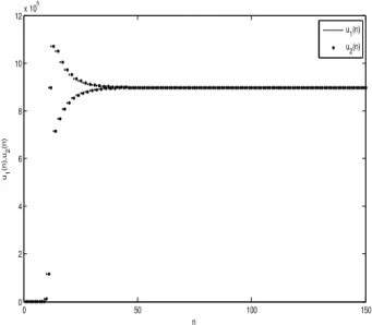
Fig. 1. Stable equilibrium point of the system(11)for parameter valuesα =0.14×10−7_,β

0=1.0005×10−6,β1=0.9855×10−7, q=0.5, h=0.15 and r=3.

Fig. 2. Flip bifurcation diagram of the system(11)for the parameter valuesα =0.14×10−7_,β

0=1.0005×10−6,β1=0.9855×10−7, q=0.5 and h=0.15.

×

(2

+

5ln(

β

1

β

1

−

α

))

β

0

−

ln(

β

1

β

1

−

α

)(2

+

ln(

β

1

β

1

−

α

))

β

₀2)

β

₁2

+

2(

α + β

0)(2

α

2(3

+

2ln(

β

1

β

1

−

α

))

+

α

(3

+

4ln(

β

1

β

1

−

α

))

β

0

−

ln(

β

1

β

1

−

α

)(2

+

ln(

β

1

β

1

−

α

))

β

₀2)

β

₁3

−

(4

α

2(

−

1

+

3ln(

β

1

β

1

−

α

))

+

2

α

(4

+

ln(

β

1

β

1

−

α

)(13

+

2ln(

β

1

β

1

−

α

)))

β

0

+

3ln(

β

1

β

1

−

α

)(2

+

ln(

β

1

β

1

−

α

))

β

₀2)

β

₁4

+

4(

−

α

(2

+

3ln(

β

1

β

1

−

α

))

+

ln(

β

1

β

1

−

α

)(2

+

ln(

β

1

β

1

−

α

))

β

0)

β

15

+

4ln(

β

1

β

1

−

α

)(2

+

ln(

β

1

β

1

−

α

))

β

₁6

]

.

Now the coefficient k, which determines the direction of the invariant curve, can be computed

k

= −

Re

[

(

1

−

2

λ) ¯λ

2 1

−

λ

ξ

11

ξ

20

]

−

1 2

|

ξ

11

|

2

_{− |}

_ξ

02

|

2

+

Re

(

_¯

λξ

21

)

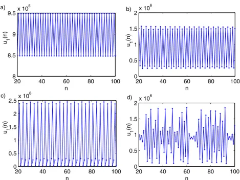
(25)

Fig. 3. Time series plot of model(11)with respect toFig. 2: (a) period-two orbit for r=3.19, (b) period-four orbit for r=3.91, (c) period-eight orbit for r=3.97, (d) chaotic for r=4.3.

where

ξ

20

=

1

8[

(

F1XX

−

F1YY

+

2F2XY

) +

i

(

F2XX

−

F2YY

−

2F1XY

)

]

,

ξ

11

=

1

4[

(

F1XX

+

F1YY

) +

i

(

F2XX

+

F2YY

)

]

,

ξ

02

=

1

8[

(

F1XX

−

F1YY

−

2F2XY

) +

i

(

F2XX

−

F2YY

+

2F1XY

)

]

,

ξ

21

=

1

16[

(

F1XXX

+

F1XYY

+

F2XXY

+

F2YYY

) +

i

(

F2XXX

+

F2XYY

−

F1XXY

−

F1YYY

)

]

.

Thus the proof of Theorem3is completed.

5. Numerical simulations

In this section, we present some numerical simulations to demonstrate the accuracy of the theoretical results obtained in Section4. Therefore, the parameter r is chosen as a bifurcation parameter and the other parameters of model are fixed. The bifurcation parameters are considered as in the following cases:

Case(i) varying r in range 2

≤

r

≤

6 and fixing

α =

0

.

14

×

10−7_,

_β

0

=

1

.

0005

×

10−6,

β

1

=

0

.

9855

×

10−7,

q

=

0

.

5 and h

=

0

.

15. From Theorem2, the critical flip bifurcation value is obtained as r∗

1

≈

3

.

18656. In this situation,

α

1

= −

1

.

57475

̸=

0 and

α

2

=

5

.

93602

×

10−15

̸=

0. Now we can say that Flip bifurcation appears around the fixed point

E∗

₌

(8

.

98432

×

10−6

_,

₈

_.

₉₈₄₃₂

_×

₁₀−6_{) for the model(11). Moreover, since}

_α

2

>

0 the period-2 orbits bifurcate from E∗

are stable (Figs. 2and3a). We note that for the above parameter values the eigenvalues of the Jacobian matrix are

λ

1

=

1

and

λ

2

=

0

.

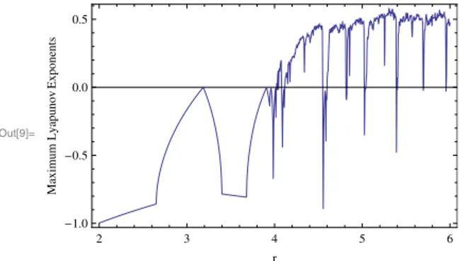
215186. In addition we calculate the maximum Lyapunov exponents correspondingFig. 2and plot inFig. 4

where some Lyapunov exponents are bigger than 0, some are smaller than 0. Therefore there exist chaotic regions and period orbits in the parametric space.

Case(ii) varying r in range 1

≤

r

≤

4 and fixing

α =

0

.

14

×

10−7_,

_β

0

=

1

.

0005

×

10−6,

β

1

=

2

.

9855

×

10−6, q

=

0

.

5 and

h

=

0

.

15. From Theorem 3, the critical Neimark–Sacker bifurcation value can be calculated as r∗

2

≈

1

.

73375. For r

=

r

∗

2,

transversality and nonresonance condition leads to d

⏐

⏐

λ

₁,₂(r)

⏐

⏐

dr

⏐

⏐

⏐

⏐

r=r∗ 2

=

0

.

398326i

̸=

0 and p(r∗ 2)

= −

0

.

660191

̸=

0

,

1,

respectively. Now Neimark–Sacker bifurcation comes out from the fixed point (2

.

5

×

105

_,

₂

_.

₅

_×

₁₀5_{) at r}∗

2

=

1

.

73375 for the

model(11)(Fig. 6). In this situation, the norm of eigenvalues of the Jacobian matrix is

|

λ

_1,2

| = |

0

.

330095

±

0

.

943948i

| =

1 and the coefficients

ξ

ij are

ξ

20

= −

5

.

31745

×

10

−7

₊

₈

_.

₄₄₁₃₁

_×

₁₀−7_i,

_ξ

11

=

1

.

10931

×

10

−9_,

_ξ

02

= −

5

.

31745

×

10−7

₋

₈

_.

₄₄₁₃₀

_×

₁₀−7_{i and}

_ξ

Fig. 4. Maximum Lyapunov exponents of the system(11)corresponding toFig. 2.

Fig. 5. Time series plot of model(11)with respect toFig. 6: (a) asymptotically stable for r=1.6, (b) quasi-periodic solution for r=1.73375, (c) quasi-periodic solution for r=1.8, (d) chaotic for r=3.4.

k

= −

9

.

98695

×

10−13_{. Therefore, a supercritical Neimark–Sacker bifurcation occurs at r}∗

2 (Fig. 6). In order to see the

chaotic dynamics, we calculate the maximum Lyapunov exponents correspondingFig. 6and plot inFig. 7. The sign of the maximum Lyapunov exponent confirms the existence of the strange attractor.

6. Results and discussion

In this work, we have considered a conformable fractional order differential equations with piecewise constant arguments model(5)for modeling bacteria population model in a microcosm. We apply a discretization process to the model(5)and obtain two dimensional discrete dynamical system(11). Thus, the fractional order parameter q is included as a new parameter into the system of difference equations. By using the Schur Cohn criterion the necessary and sufficient stability conditions of the model according the parameter r is obtained and given in Theorem 1. The parameter values are taken in [4] in terms of consistency with the biological facts as

α =

0

.

14

×

10−7_,

_β

0

=

1

.

0005

×

10−6,

β

1

=

0

.

9855

×

10−6,

q

=

0

.

5 and h

=

0

.

15 and initial condition for bacteria population is nearly 10−4 _{(cells/ml). Theorem 1 gives two}

stability regions according the bacteria population growth rate (r). The first stability region obtained from Theorem1(i) is r

<

3

.

18656

=

r∗

1. If bacteria population growth rate is chosen r

=

3, then the bacteria population increase and

eventually reaches to stable equilibrium point 8

.

98432

×

105 _{that is homogeneous bacteria distributions (Fig. 1). Let}

Fig. 6. Neimark–Sacker bifurcation diagram of the system(11)forα =0.14×10−7_,β

0=1.0005×10−6,β1=2.9855×10−6, q=0.5 and h=0.15.

Fig. 7. Maximum Lyapunov exponents of the system(11)corresponding toFig. 6.

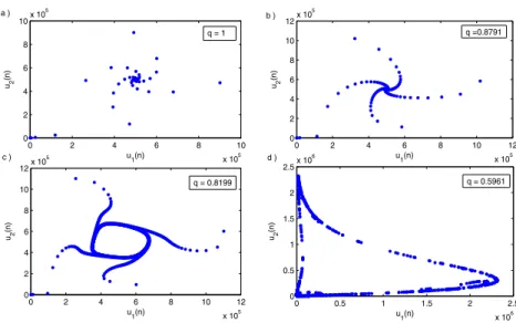
Fig. 8. Phase portraits for different values of q for the system(11).

By using the center manifold theorem and the bifurcation theory we show that the discrete system(11)undergoes both a Flip bifurcation and a Neimark–Sacker bifurcation around the positive equilibrium point. If bacteria population growth rate passes a threshold value r∗

occurs for a bacteria population that is inhomogeneous spatial population distributions (Figs. 2,3,4). From these figures, we observe the existence many attractors (e.g., steady state, period-2 orbit, period-4 orbit, period-8 orbit, chaos etc.) with the variation parameter r. Therefore the model is sensitive to initial conditions and therefore model (11) is multistable system. In addition, for r₂∗

=

1

.

73375 a stable limit cycle is formed around the equilibrium point as a result of Neimark– Sacker bifurcation (Figs. 5,6,7). From these figures, we also observe the existence quasi-periodic solution and chaos for the model(11)with the variation parameter r. This is another indication that the system is multistable. Multistable system is also seen in study [40,41].

On the other hand, the effect of the change of fractional order derivative parameter q on system(11)is illustrated in

Fig. 8. This figure shows that the stable behavior of the system is destabilizing when decreasing the parameter q.Fig. 8

demonstrate phase portraits of the model and clearly depicts how a smooth invariant circle bifurcates from the stable equilibrium point (2

.

5

×

105

,

2

.

5

×

105). The equilibrium point of the model is stable for q

<

0

.

8199 (Fig. 8a–b), that is loses its stability q

=

0

.

8199 through the Neimark–Sacker bifurcation (Fig. 8c), and that an invariant circle appears when the parameter q exceeds 0.8199. After this, its radius becomes larger with the decrease of parameter q and chaotic attractor is formed around the equilibrium point (Fig. 8d).

Our model (5) is a more general model than model (4) in that it includes local fractional order derivative q and discretization parameter h. We note that if we choose q

=

1 and h

=

1 in model(5), the model is reduced to model

(4). However, since model(5)is a local fractional order, it includes local memory effects for a bacteria population that cannot be reflected by integer order model(4). Therefore, the model exhibits richer dynamic behaviors than the model

(4)according to the different states of the local fractional order parameter q. In our model, Neimark–Sacker bifurcation occurs around the positive equilibrium point for q

=

0

.

8199 (Fig. 8). It is not possible to observed this situation in model

(4)because it does not include local fractional order parameter q. This is an expected result when we compare fractional order dynamical systems with integer order counterpart.

7. Conclusion

In this study, we consider a bacteria population model consisting of conformable fractional order differential equation with piecewise constant arguments. Since the model(5)is a local fractional order, it contains the local memory effect. This shows the advantage of our model compared to model(4)formed by ordinary differential equations. We also use piecewise constant arguments including control parameter h which represents the delay effect in the population. Thus, discretization parameter h take control the length of the subintervals

[

nh

,

(n

+

1)h) that give us to controlling dynamical behavior of the discrete model(11). It is observed that the discrete model has quite rich dynamic behaviors such as period-2, period-4, period-8, quasi-periodic solutions and chaos according to the change of parameter r which demonstrates bacteria population growth rate. Periodic solutions lead to flip bifurcation and quasi periodic solutions cause to Neimark– Sacker bifurcation, that resulting in chaotic behavior. Due to the increase of the parameter r, quasi-periodic solutions first lead to damped oscillatory solutions, followed by stable limit cycles and then chaotic behaviors. These dynamic behaviors explain some biological phenomena such as homogeneous and inhomogeneous spatial population distributions for the bacteria population and provide a recipe for controlling the bacteria population. In addition, changing of fractional parameter q in the system show that local memory effect causes significant structural changes such as Neimark–Sacker bifurcation and chaos in dynamical behavior of the model.

Declaration of competing interest

The authors declare that they have no known competing financial interests or personal relationships that could have appeared to influence the work reported in this paper.

References

[1] R.J. Beyers, H.T. Odum, Ecological Microcosm, Springer Verlag, New York, 1993. [2] E.P. Odum, Trends expected in stressed ecosystems, Bioscience 35 (1985) 419–422.

[3] J.W. Fleeger, K.R. Carman, R.M. Nisbet, Indirect effects of contaminants in aquatic ecosystems, Sci. Total Environ. 317 (2003) 207–233. [4] I. Ozturk, F. Bozkurt, F. Gurcan, Stability analysis of a mathematical model in a microcosm with piecewise constant arguments, Math. Biosci.

240 (2012) 85–91.

[5] G.F. Gause, The Struggle for Existence, Williams and Wilkins, Baltimore, 1934.

[6] A.A. Grigoryan, D.R. Jalique, P. Medihala, et al., Bacterial diversity and production of sulfide in microcosms containing uncompacted bentonites, Heliyon 4 (2018) e00722.

[7] T.H. Hevroy, A.L. Golz, E.L. Hansen, et al., Radiation effects and ecological processes in a freshwater microcosm, J. Environ. Radioact. 203 (2019) 71–83.

[8] F. Centler, I. Fetzer, M. Thullner, Modeling population patterns of chemotactic bacteria in homogeneous porous media, J. Theoret. Biol. 287 (2011) 82–91.

[9] R.M. May, Biological populations obeying difference equations : Stable points, stable cycles, and chaos, J. Theoret. Biol. 51 (1975) 511–524. [10] R.M. May, Simple mathematical models with very complicated dynamics, Nature 261 (1976) 459–467.

[11] F.C. Hoppensteadt, Cambridge Studies in Mathematical Biology: Mathematical Methods of Population Biology, Cambridge University Press, Cambridge, 2004.

[13] Z. Zheng, H. Dai, A new fractional equivalent linearization method for nonlinear stochastic dynamic analysis, Nonlinear Dynam. 91 (2) (2018) 1075–1084.

[14] A. Ortega, J.J. Rosales, J.M. Cruz-Duarte, et al., Fractional model of the dielectric dispersion, Optik 180 (2019) 754–759.

[15] M.S. Hashemi, Invariant subspaces admitted by fractional differential equations with conformable derivatives, Chaos Solitons Fractals 107 (2018) 161–169.

[16] T.M. Atanackovic, B. Stankovic, An expansion formula for fractional derivatives and its application, Fract. Calc. Appl. Anal. 7 (2004) 365–378. [17] A. Atangana, J.F. Gomez-Aguilar, Decolonisation of fractional calculus rules: Breaking commutativity and associativity to capture more natural

phenomena, Eur. Phys. J. Plus 133 (2018) 166.

[18] Z. Zheng, W. Zhao, H. Dai, A new definition of fractional derivative, Int. J. Non-Linear Mech. 108 (2019) 1–6.

[19] L. Bolton, A.H.J.J. Cloot, S.W. Schoombie, et al., A proposed fractional-order Gompertz model and its application to tumour growth data, Math. Med. Biol. 32 (2) (2015) 187–209.

[20] S. Qureshi, A. Yusuf, Fractional derivatives applied to MSEIR problems: Comparative study with real world data, Eur. Phys. J. Plus 134 (2019) 171.

[21] A. Atangana, I. Koca, Chaos in a simple nonlinear system with Atangana–Baleanu derivatives with fractional order, Chaos Solitons Fractals 89 (2016) 447–454.

[22] R. Khalil, M. Al Horani, A. Yousef, et al., A new definition of fractional derivative, J. Comput. Appl. Math. 264 (2014) 65–70.

[23] V.F. Morales-Delgado, J.F. Gomez-Aguilar, et al., Fractional conformable derivatives of Liouville–Caputo type with low-fractionality, Physica A 503 (2018) 424–438.

[24] T. Abdeljawad, On conformable fractional calculus, J. Comput. Appl. Math. 279 (2015) 57–66.

[25] S. Kartal, F. Gurcan, Discretization of conformable fractional differential equations by a piecewise constant approximation, Int. J. Comput. Math. (96) (2019) 1849–1860.

[26] S. Kartal, F. Gurcan, Stability and bifurcations analysis of a competition model with piecewise constant arguments, Math. Methods Appl. Sci. 38 (2015) 1855–1866.

[27] F. Gurcan, S. Kartal, I. Ozturk, F. Bozkurt, Stability and bifurcation analysis of a mathematical model for tumor–immune interaction with piecewise constant arguments of delay, Chaos Solitons Fractals 68 (2014) 169–179.

[28] S. Kartal, Multiple bifurcations in an early brain tumor model with piecewise constant arguments, Int. J. Biomath. 11 (4) (2018) 1850055. [29] S. Kartal, Flip and Neimark–Sacker bifurcation in a differential equation with piecewise constant arguments model, J. Difference Equ. Appl. 23

(4) (2017) 763–778.

[30] F. Kangalgil, Neimark–Sacker bifurcation and stability analysis of a discrete-time prey–predator model with Allee effect in prey, Adv. Differential Equations (2019)http://dx.doi.org/10.1186/s13662-019-2039-y.

[31] F. Kangalgil, Flip bifurcation and stability in a discrete-time prey-predator model with allee effect, Cumhur. Sci. J. 40–1 (2019) 141–149. [32] Y.D. Ji, L. Lai, S.C. Zhong, L. Zhang, Bifurcation and chaos of a new discrete fractional-order logistic map, Commun. Nonlinear Sci. Numer. Simul.

57 (2018) 352–358.

[33] K. Nosrati, M. Shafiee, Fractional-order singular logistic map: Stability, bifurcation and chaos analysis, Chaos Solitons Fractals 115 (2018) 224–238.

[34] A.A. Khennaoui, A. Ouannas, S. Bendoukha, et al., On fractional-order discrete-time systems: Chaos, stabilization and synchronization, Chaos Solitons Fractals 119 (2019) 150–162.

[35] S. Zhang, Y. Zeng, Z. Li, Chaos in a novel fractional order system without a linear term, Internat. J. Non-Linear Mech. 106 (2018) 1–12. [36] C.H. Gibbons, M.R.S. Kulenovic, G. Ladas, H.D. Voulov, On the trichotomy character of xn+1=(α + βxn+γxn−1)/(A+xn), J. Difference Equ.

Appl. 8 (2002) 75–92.

[37] M. Zhao, Z. Xuan, C. Li, Dynamics of a discrete-time predator–prey system, Adv. Differential Equations 2016 (2016) 191. [38] P. Chakraborty, S. Poria, Extreme multistable synchronisation in coupled dynamical systems, J. Phys. 93 (2019) 19.

[39] J. Guckenheimer, P. Holmes, Nonlinear Oscillation Dynamical Systems and Bifurcations of Vector Fields, Springer-Verlag, New York, 1983. [40] P. Chakraborty, A scheme for designing extreme multistable discrete dynamical systems, J. Phys. 89 (2017) 41.

[41] J. Wang, Y. Li, S. Zhong, X. Hou, Analysis of bifurcation, chaos and pattern formation in a discrete time and space Gierer Meinhardt system, Chaos Solitons Fractals 118 (2019) 1–17.