YAŞAR UNIVERSITY
GRADUATE SCHOOL OF NATURAL AND APPLIED SCIENCES
MASTER THESIS
CONTROL OF A MULTI-SERVER MAKE-TO-STOCK
PRODUCTION SYSTEM WITH SETUP COSTS
Sinem ÖZKAN
Thesis Advisor: Asst. Prof. Dr. Önder BULUT
Department of Industrial Engineering
Presentation Date: 25.01.2016
Bornova-İZMİR 2016
iii
ABSTRACT
CONTROL OF A MULTI-SERVER MAKE-TO-STOCK
PRODUCTION SYSTEM WITH SETUP COSTS
ÖZKAN, Sinem MSc in Industrial Engineering Supervisor: Asst. Prof. Dr. Önder BULUT
February 2016, 61 pages
This study considers production and inventory control problems for a make-to-stock queue with production setup costs, several customer classes and lost sales. At any system state, production decision is to specify whether to activate new production channels or to continue with the currently active ones. If the decision is to activate new channels, a fixed/setup cost is incurred per channel. At the decision epochs where the system experiences demand from any customer class, the controller should also decide whether to satisfy the arriving demand or to reject it. The literature of the control of make-to-stock queues is extended by considering fixed system costs and multiple servers at the same time. Firstly, the structure of the optimal production and rationing policies are characterized and then new/alternative policies that have well-defined structures and are easier to apply are proposed. Numerical and theoretical studies are carried out to assess the performances of the proposed policies. The expected average cost of the optimal production policy for the single-server make-to-stock queue is obtained conducting a renewal analysis.
Keywords: Fixed/Setup cost, inventory and production control, stock rationing, make-to-stock, multiple servers, optimal control.
iv
ÖZET
PARALEL ÜRETİM KANALLI VE HAZIRLIK MALİYETLİ STOĞA-ÜRETİM SİSTEMLERİNİN KONTROLÜ
Sinem ÖZKAN
Yüksek Lisans Tezi, Endüstri Mühendisliği Bölümü Tez Danışmanı: Yrd. Doç. Dr. Önder BULUT
Şubat 2016, 61 sayfa
Bu çalışmada paralel üretim kanalları olan, birden çok müşteri sınıfına sahip, hazırlık ve kayıp satış maliyetli Stoğa-üretim sistemleri için üretim ve stok tayınlama kontrol problemleri ele alınmaktadır. Üssel dağılıma sahip üretim zamanı içeren bu sistem 𝑀 /𝑀 /s stoğa-üretim kuyruk modeli olarak incelenmektedir. Herhangi bir sistem-durumunda, üretim kararı ya aktif olan üretim kanal sayısının arttırılmasını ya da aktif olan kanal sayısı ile devam edilmesini belirtir. Karar anlarında, eğer herhangi bir müşteri sınıfından talep gelirse, tayınlama kararı ya gelen talebin karşılanmasını ya da reddedilmesini sağlar. Bu çalışmayla, hazırlık maliyetli Stoğa-üretim sistemlerini şimdiye kadar tek bir üretim kanalıyla modelleyen çalışmaları içeren teknik yazına önemli katkıda bulunulmaktadır. Öncelikle, en iyi üretim ve tayınlama politikalarının yapıları belirlenmiş, daha sonra ise en iyi politikalara benzer ve uygulaması daha kolay olan alternatif politikalar sunulmuştur. Sunulan politikaların performanslarının ölçülebilmesi için nümerik ve teorik çalışmalar yapılmıştır. Tek kanallı sistem için en iyi üretim politikasının beklenen ortalama maliyeti hesabı için Yenileme Ödül Teoremi kullanılmıştır.
Anahtar sözcükler: Sabit/Hazırlık maliyeti, envanter ve üretim kontrol, stok tayınlama, Stoğa-üretim, paralel üretim kanalları, en iyi kontrol.
v
ACKNOWLEDGEMENTS
Firstly, I would like to express my sincere gratitude to my supervisor Asst. Prof. Dr. Önder Bulut for the continuous support of my graduate study and related research, for his patience, motivation, and immense knowledge. His guidance helped me in all the time of research and writing of this thesis.
Besides my supervisor, I would like to thank Prof. Dr. M. Murat Fadıloğlu for his insightful comments and encouragement.
I thankfully acknowledge the support of TUBITAK - Turkish Technological and Scientific Research Institute for during my master period. This research is a part of a project supported by TUBITAK project number 213M355.
The last but not the least, I would also like to thank my parents, sister and spouse. They were always there supporting me and encouraging me with their best wishes.
Sinem ÖZKAN İzmir, 2016
vi
TEXT OF OATH
I declare and honestly confirm that my study, titled “Control of a Multi-Server Make-to-Stock Production System with Setup Costs” and presented as a Master’s Thesis, has been written without applying to any assistance inconsistent with scientific ethics and traditions, that all sources from which I have benefited are listed in the bibliography, and that I have benefited from these sources by means of making references.
vii TABLE OF CONTENTS Page ABSTRACT iii ÖZET iv ACKNOWLEDGEMENTS v TEXT OF OATH vi
TABLE OF CONTENTS vii
INDEX OF FIGURES ix
INDEX OF TABLES x
INDEX OF SYMBOLS AND ABBREVIATIONS xii
1 INTRODUCTION 1
2 LITERATURE REVIEW 6
3 MODEL 12
3.1 Dynamic Programming Formulation 13
3.2 Characterization of the Optimal Policies 14
3.3 The Impact of the System Parameters on the Optimal Policies 20
4 THE PROPOSED PRODUCTION AND RATIONING POLICIES 29
viii
The Proposed Production Policy 1 30
4.1.1
The Behaviour of Proposed Production Policy 1 31 4.1.1.1
The Proposed Production Policy 2 33
4.1.2
The Behaviour of Proposed Production Policy 2 34 4.1.2.1
Continuous Time Markov Chain Analysis for PP2 36 4.1.2.2
The Proposed Production Policy 3 38
4.1.3
The Behaviour of Proposed Production Policy 3 39 4.1.3.1
Continuous Time Markov Chain Analysis 43 4.1.3.2
Renewal Analysis for 𝑀/𝑀/1 46
4.1.3.3
4.2 The Proposed Rationing Policy 52
The Behaviour of Proposed Rationing Policy 53 4.2.1.1
5 CONCLUSION 57
REFERENCES 58
CURRICULUM VITEA 61
ix
INDEX OF FIGURES
Figure 1.1 A Supply Chain Example ... 3
Figure 3.1 The Pseudo-code of Value Iteration Algorithms... 16
Figure 4.1 State Transition Diagram ... 37
Figure 4.2 The Cost Differences of Optimal and Proposed Policies as K increases .. 41
Figure 4.3 The Cost Differences of Optimal and Proposed Policies as s increases ... 42
Figure 4.4 X*=X**=6 State Transition Diagram ... 43
Figure 4.5 X*=1, X**=6 State Transition Diagram ... 44
Figure 4.6 X*=4, X**=6 State Transition Diagram ... 44
Figure 4.7 (S,s) Policy ... 45
Figure 4.8 A sample state diagram ... 50
Figure 4.10 The Impact of the ratio of p ... 55
x
INDEX OF TABLES
Table 2.1 Summary of the Related Literature on Production-Inventory Control ... 11
Table 3.1 Optimal Production Decisions up when s=1... 17
Table 3.2 Optimal Production Decisions up ... 18
Table 3.3 Optimal Inventory Rationing Policy for Class 1 ... 19
Table 3.4 Optimal Inventory Rationing Policy for Class 2 ... 19
Table 3.5.Optimal Production Decisions Under Discounted Cost Criterion ... 20
Table 3.6 Optimal Rationing Decisions Under Discounted Cost Criterion... 20
Table 3.7 The Impact of the Fixed Cost on Optimal Decisions ... 21
Table 3.8 The Impact of Number of Servers on Optimal Decisions ... 22
Table 3.9 The Impact of Holding Cost on Optimal Decisions ... 23
Table 3.10 The Impact of Production Rate on Optimal Decisions ... 24
Table 3.11 The Impact of Demand Rates on Optimal Decisions ... 25
Table 3.12 The Impact of Lost Sales Costs on Optimal Decisions ... 26
Table 4.1 The Impact of Fixed Cost on Optimal Production and PP1 Policies... 32
Table 4.2 The Impact of Fixed Cost on Optimal, PP1 and PP2 Policies ... 34
Table 4.3 The Impact of Number of Servers on Optimal, PP1 and PP2 Policies ... 35
xi
Table 4.5 Optimal and Proposed Policy 3 Production Decisions for larger 𝑠 ... 40
Table 4.6 Comparison of Production Policies in terms of their structures ... 42
Table 4.7 CPU Times of MDP & RA ... 51
Table 4.8 Optimal, Static, FCFS, and The Proposed Rationing Policy Decisions ... 54
xii
INDEX OF SYMBOLS AND ABBREVIATIONS
Symbols Explanations
K Fixed cost
s Number of available servers
h Holding cost per unit
𝑐𝑖 Lost sales cost of demand class 𝑖
𝜆𝑖 Demand rate of class 𝑖
𝜇 Production rate
𝛼 Discount rate
𝑋(𝑡) Inventory level at time 𝑡
𝑌(𝑡) Number of active channels at time 𝑡
𝑢𝑝(𝑡) The production decision at time 𝑡
𝑢𝑟(𝑡) The rationing decision at time 𝑡
Abbreviations
xiii
BSP Base-Stock Policy
MDP Markov Decision Process
RA Renewal Analysis
PPP1 Proposed Production Policy 1
PPP2 Proposed Production Policy 2
1
1 INTRODUCTION
The joint production and inventory control arises when there is limited number of production channels and the underlying system is make-to-stock. In general, production controllers desire to produce the ideal amount of products to meet random demand so as to balance holding and shortage costs. Today, in addition to these features, most of the production systems experience demands from the several different customer classes. Differentiation among customer classes is based on either the shortage costs or the service level requirements. If the customers have different shortage costs/service level requirements, reservation of inventory gains importance at this stage. It is a good strategy to reserve the inventory by not satisfying demand from lower priority classes in anticipation of future demand from the higher priority classes.
In this thesis, we consider the problem of production control and stock rationing of a single-item, make-to-stock production facility with parallel production channels and several demand classes. Contrary to the vast majority of the literature, this problem, which is considered in the lost sales environment, is considered under existence of fixed production cost. There are two essential decisions should be jointly addressed for managing such a system: The first one is the production control decision that dictates when to start production and how much to produce i.e., how many production channels should be activated. The second control is concerned with inventory rationing. Stock-rationing is mainly to reserve inventory for the future demand from more valuable demand classes by rejecting demands from less valuable demand classes. Thus, the joint management of production and inventory control has a huge potential to decrease the total production and inventory related costs.
In the most general setting, this joint problem is hard to solve and can be even intractable. The system-state should dynamically keep track of the number of outstanding production orders, the indices of the active channels (processing time distributions might be different for different channels), and the age information (or
2
the remaining completion times) of all these random number of orders. Hence, the structure of the unknown optimal policy would be highly dynamic and would not possess a systematic behaviour for all practical purposes. Thus, in addition to characterize the optimal production and rationing policies as much as possible, introducing and analyzing new/alternative policies which are well-performing and have well-defined structures would be very beneficial for both literature and practice.
Although the general setting is too complex to analyze and we make some assumptions, in our model we still allow parallel channels which is not typical in the literature. That is, we have the flexibility of changing the number of channels/servers. This provides us to consider our problem under different settings that can be grouped in two main categories: Capacitated and Uncapacitated systems. For Capacitated
production-inventory systems, the number of production channels is limited and most
of the time all of them are utilized. The extreme of such a system has only a single production channel. In the production control literature, the optimal production policy for such a single-server system is to produce until a threshold inventory level and stop the production (Ha (1997a, 1997b)) which is the well-known Base-Stock Policy. Moderate values of number of production channels are analyzed as parallel production channels. For this case, the optimal production and rationing policies are more dynamic and the optimal rationing policy is state-dependent threshold type (Bulut and Fadıloğlu (2011)). As the number of servers approaches to infinity, capacitated production systems converge to Uncapacitated systems: At any time needed, a new order can be triggered. Hence, the infinite number of channels helps us to analyze typical inventory systems having ample supply.
Another problem addressed in this study is allocation of inventory among several demand classes from a common stock pool. The common stock pool provides not to have excessive inventory and to use system resources effectively. In inventory systems, rationing is a well-known strategy and is observed frequently in real life. Also, customer differentiation is often observed in different service industries such as hotels, banks or airline management etc. While we differentiate customers to manage
3
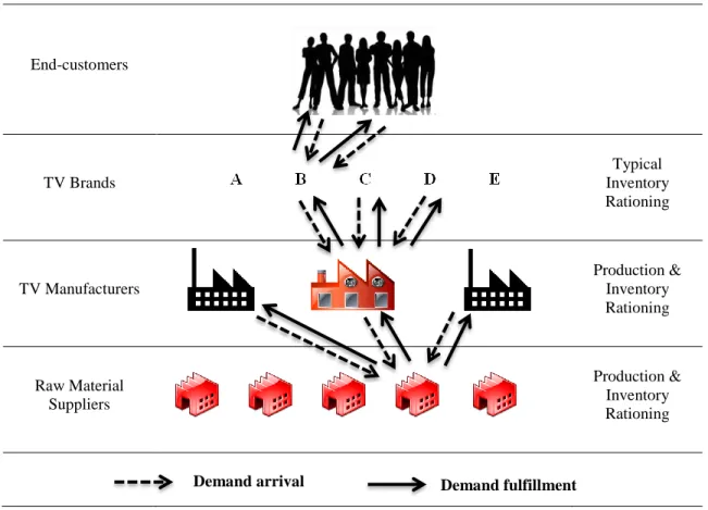
the inventory, service industry uses customer differentiation strategy in queuing and revenue management. End-customers TV Brands Typical Inventory Rationing TV Manufacturers Production & Inventory Rationing Raw Material Suppliers Production & Inventory Rationing
Figure 1.1 A Supply Chain Example
In order to better understand the problem, let us consider the following supply chain example depicted in Figure 1.1 where we can face with our problem at different echelons: Suppose there is a television manufacturer that produces televisions and gives services to many different brands or companies. It has parallel production lines that produce with a fixed cost to a common buffer stock. All the items in the buffer stock are identical and semi-finished. After a demand occurs, work in process is pulled and differentiated based on different requests of the customers. This strategy is known as Delayed Differentiation in the literature (Lee and Tang (1997)). TV manufacturer has many customers and each of them order televisions that have different priorities. For instance, one of the customers of the manufacturer might be the world’s number one and hence this specific brand would have the highest priority for the TV manufacturer because lost sales cost of this brand would be the highest.
4
We can also consider the lower echelon of the supply chain from our problem perspective. In order to trigger the production, TV manufacturer needs raw materials. Hence, the TV manufacturer has raw material suppliers to supply them. If we consider one of these suppliers, our TV manufacturer is one of the customers of this raw material supplier. The raw material supplier should also have its own production and rationing strategies to meet demands from several TV manufacturers. On the other hand, at the higher echelon of the supply chain, end-customer demands come to any brand which is one of the customers of TV manufacturer. This company has to decide to satisfy or not to satisfy the demand based on customer differentiation. This decision is related with typical inventory rationing. Occurrence of end-customer demand leads to order the televisions from TV manufacturer. Then, our TV manufacturer starts to the differentiation of semi-products to satisfy the demand of the company. As seen from this example the problem we consider in this thesis can be experienced at different levels of the supply chains of many industries.
In this thesis, we first characterize the structural properties of the optimal production and rationing policies for a single product, multi-server, make-to-stock production system with fixed production costs, multiple customer classes and lost sales. We then propose well-performing alternative policies and conduct the performance analyses. In order to analyze such a system we assume the following: Demands from different customer classes are generated according to independent stationary Poisson processes. Processing times at each identical server are independent Exponential random variable with rate 𝜇. Hence, we model production-inventory system as an 𝑀/𝑀/𝑠 make-to-stock queue. In this model, at any system state the controller decides the number of new channels/servers that should be activated in conjunction with the rationing decision. The cancellation of previously placed production orders is not permitted.
The remainder of this thesis is organized as follows: We review the related literature in Chapter 2. In Chapter 3 we present problem formulation and numerical characterization of the optimal production and rationing policies. In Chapter 4 we
5
propose new policies and compare their structure, applicability and performances with the optimal ones. In this chapter, we also provide the renewal analysis for 𝑀/𝑀/1 make-to-stock queue. We finally provide an overall summary of the thesis and discuss possible directions for future research in Chapter 5.
6
2 LITERATURE REVIEW
The related literature can be classified into two categories from both chronological and methodological perspectives. The first category is defined as the literature published before Ha (1997a) and the second category is defined as the literature published after Ha (1997a). In earlier studies such as Sobel (1968), Gavish and Graves (1980,1981), Graves and Keilson (1981), single-server, single-demand-class settings with setup costs are considered and analyzed using queueing theory techniques. In the second category, starting with Ha (1997a), in almost all the studies, problem is attacked using Markov Decision Process (MDP) analysis techniques. Interestingly, all such studies assume that setup/startup cost is zero. On the other hand, in this second research stream, studies consider more than single customer class and accordingly rationing policies. In parallel with the first category, the studies in this second category also assume a single processing channel with only one exception which is Bulut and Fadıloğlu (2011). Mainly, our study extends the literature before Ha (1997a) by increasing the number of production channels and the literature after Ha (1997a) by considering the fixed cost per each active production channel.
The earlier studies including fixed costs start with Sobel (1968) and analyze queueing systems with a single server. Sobel (1968) analyzes a service system under general service time distributions and general arrival processes with fixed start-up and shut-down costs. He presents a queue control strategy based on a given cost structure. He proves that two-critical-number policy, which resembles the (𝑠, 𝑆) policy for the typical inventory systems, is the optimal service policy. This policy includes two control variables denoted by 𝑋∗ and 𝑋∗∗ such that 𝑋∗ < 𝑋∗∗. If queue length is less than or equal to 𝑋∗, service is not provided until queue length reaches to 𝑋∗∗ , whereupon service starts and continues until queue length drops to 𝑋∗, again. Based
on the work of Sobel (1968), Gavish and Graves (1980) reconsiders a similar problem in a production-inventory setting. Actually, the queue length in Sobel’s study correspond to the number of backorders in this study. They assume unit Poisson demand arrivals, constant demand size and fixed setup cost for production. If demand is rejected, it is backlogged. They model their system as 𝑀/𝐷/1 queue. They derive
7
cost expressions and propose an efficient search procedure to find the optimal policy parameters. Gavish and Graves (1981) extends the work of Gavish and Graves (1980) by allowing general service times. They generate a procedure to find the steady-state probabilities of each inventory level and used this procedure to search optimal 𝑋∗ and
𝑋∗∗ control levels. Graves and Keilson (1981) extends the previous works by
including an exponential random variable which is the size of the demand requests. They generate a compensation method for the backordering case that finds a closed-form expression for the expected system cost. They used this procedure to find optimal 𝑋∗ and 𝑋∗∗ control levels. If inventory is less than 𝑋∗, production channel is
triggered to start with a fixed setup cost and continues until inventory level reaches to 𝑋∗∗. While the production is continuing, the fixed setup cost is not incurred. If
inventory level hits to 𝑋∗∗, the production is turned off and stays off until inventory
level drops to below 𝑋∗.
Tijms (1980) studied the similar system with Poisson demands and random service times. The optimal control values are found by using Semi-Markov decision process techniques. Besides, the model also includes the time taken to activate the production channels. Altiok (1986) considers a system with compound Poisson demands and phase-type service times. Steady-state probabilities are calculated for each inventory level. This study can be adapted to both lost sales and backordering environments. Another important study is Lee and Srinivasan (1989) considers a system includes single item and a production channel with fixed start-up costs. The processing time has a general distribution and each demand arrives according to Poisson process. If there is not enough inventory, demands are backordered. The importance of this article is enabling to calculate the cost function by not calculating the steady-state probabilities. They succeed to achieve this using a renewal anaysis. Later on, Lee and Srinivasan (1991) extended the previous work by adding compound Poisson structure.
Ha (1997a) is the first to model the problem by using Markov Decision Process techniques. The setting includes an exponential server with no fixed cost, multiple
8
demand classes with Poisson arrivals and lost sales. He shows that the optimal production policy is Base-stock policy for such a system. Also, the stock rationing problem in production environment was analyzed first by Ha (1997a) and he shows that a static threshold level policy is optimal for rationing. A stationary analysis is performed of a system with two demand classes. The comparisons between the performances of optimal rationing policy and FCFS policy are also conducted.
Ha (1997b) considered the same system with two demand classes, exponential production times and backordering. He defines the system-state with two variables. The first variable denotes to the inventory level. For zero and negative values of the first variable, it corresponds to the number of class 1 backorders. For positive values of the first variable, it corresponds to the units of inventory and the second variable denotes the number of class 2 backorders. He shows the optimal policies are characterized by a single monotone switching curve. Optimal production policy is Base-stock and optimal rationing policy is applied by a threshold level. Vericourt et al. (2002) included multiple demand classes to the work of Ha (1997b). The characterization of the optimal rationing policy is provided and an efficient algorithm is generated to compute optimal control parameters which are the optimal rationing levels for each demand class.
Bulut and Fadıloğlu (2011) included multiple production channels to the work of Ha (1997a). Until our study, this research was the unique study that considers multi-servers. They characterized the properties of the optimal cost function, the optimal production and rationing policies. The optimal production policy is a state-dependent base-stock policy, and the optimal rationing policy is threshold type.
Erlangian service times in the lost sales and backordering environments were considered by Ha (2000) and Gayon, Vericourt and Karaesmen (2009). Ha (2000) analyzes the optimal production and rationing policies in lost sales environment and defines a work storage level as a state of the system. Work storage level is number of completed production stages and has information about inventory level and the status of the production. There are optimal threshold levels for both production and
9
rationing. If work storage level is less than a pre-determined level, the optimal is to produce until the work storage level hits to target value. Also, the work storage level is higher than target level, the optimal rationing decision is to satisfy the arrival demand class. Gayon et al. (2009) also considers the previous model in backordering environment. They show that work-storage type policy is optimal for rationing by providing a partial characterization.
Lee and Hong (2003) extends the work of Ha (1997a, 2000) by integrating setup cost to a production system with multi demand classes and lost sales. Demands arrive according to a Poisson process and processing time for each single item follows a 2-phase Coxian distribution. This system is modeled as continuous time Markov chain and the steady state probabilities are calculated by an efficient algorithm. For given optimal (𝑠, 𝑆) obtained, they propose a heuristic algorithm to determine the threshold levels for stock rationing. Recently, Pang et al. (2014) study a system with several customer classes in a lost sales make-to-stock production environment with single channel and no fixed costs. In this study, they allow batch demand and consider general, phase-type and Erlang processing time distributions. It is shown that the optimal rationing policies are time-dependent threshold type.
The studies in stock rationing area were started in the 1960s. Most of the studies are for classical inventory systems. Critical level rationing is the first introduced by Veinott (1965). The model includes zero lead times and backordering costs. His model provides different service levels to several demand classes in periodic inventory system. These service levels provide to allocate on-hand inventory among distinct demand classes. Under the static rationing policy, Nahmias and Demmy (1981) consider two demand classes with Poisson arrivals and apply static rationing with zero lead time. The derivations to find expected number of backorders are performed. This study is the first to analyze stock rationing in continuous time. Deshpande et al. (2003) extend the work of , Nahmias and Demmy (1981) by providing the flexibility to number of outstanding orders. Arslan et al. (2007) consider a system with multiple demand classes, Poisson arrivals and constant lead
10
time. They also provide a heuristic to obtain optimal rationing levels. Fadiloglu and Bulut (2010) proposes a dynamic rationing policy for continuous-review inventory systems. Here, dynamic rationing implies that the rationing levels are functions of the number of outstanding orders and their ages. In general, the optimal rationing policy would be of dynamic type. However, for sake of analysis most of the studies in inventory rationing literature assume static rationing levels.
Liu, Feng and Wong (2014) analyze different inventory rationing policies for an inventory system includes two demand classes. The steady-state probabilities are calculated and the performances of policies are explored. A heuristic algorithm is generated to find the optimal values of control variables. Wang and Tang (2014) address an inventory system with multiple demand classes of backorder and lost sales type. The penalty costs of backorders changes as time progresses. Hence, the importance of demand classes change with time. They analyze a dynamic rationing policy and model a Markov decision process (MDP) to observe optimal dynamic threshold levels for inventory rationing. The optimal rationing policy is shown to be a myopic base stock policy and dynamic rationing policy. A heuristic dynamic inventory policy is introduced to facilitate the solution of the complex problem. Liu and Zhang (2015) analyze an inventory system with two demand classes, Poisson demand with holding and penalty costs in backordering environment. They introduce an efficient method to obtain closed-form expressions for the dynamic threshold levels to overcome the computational complexity.
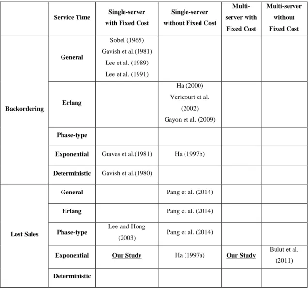
We would like to conclude the literature of the control of production-inventory systems with Table 2.1 that summarizes the related milestone works. In this table, the studies are classified on number of servers and fixed cost value. Our problem is closely related to the works of Bulut and Fadıloğlu (2011) and Graves and Keilson (1981). We extend the work of Bulut and Fadıloğlu (2011) by adding the fixed production cost per channel and the work of Graves and Keilson (1981) to multi-server case using a two-dimensional state space.
11
Table 2.1 Summary of the Related Literature on Production-Inventory Control
Service Time Single-server with Fixed Cost
Single-server without Fixed Cost
Multi-server with Fixed Cost Multi-server without Fixed Cost Backordering General Sobel (1965) Gavish et al.(1981) Lee et al. (1989) Lee et al. (1991) Erlang Ha (2000) Vericourt et al. (2002) Gayon et al. (2009) Phase-type
Exponential Graves et al.(1981) Ha (1997b)
Deterministic Gavish et al.(1980)
Lost Sales
General Pang et al. (2014)
Erlang Pang et al. (2014)
Phase-type Lee and Hong
(2003) Pang et al. (2014)
Exponential Our Study Ha (1997a) Our Study Bulut et al.
(2011)
12
3 MODEL
In this chapter, we first characterize the structural properties of the optimal production and rationing policies for a single product, identical-multi-server, make-to-stock production with fixed production costs, multiple customer classes and lost sales. In order to analyze such a system we assume following: Demands from customer class 𝑖 are generated according to a stationary Poisson process with rate 𝜆𝑖, 𝑖 ∈ {1,2, … , 𝑁} and production times are independent Exponential random variables with mean 1/𝜇. Each demand class is prioritized by its lost sales cost 𝑐𝑖 that incurred when class 𝑖 demand is not satisfied. Without loss of generality, it is assumed that 𝑐1 ≥ 𝑐2 . .. ≥ 𝑐𝑁. The fixed cost to activate a new server is 𝐾, the holding cost per item in the inventory is ℎ, the discount rate is 𝛼 and order-cancellation is not allowed. If the order-cancellation is allowed, we have a flexibility to cancel all previously placed production orders. If almost all available production channels are active until the inventory hits a specific level and one of the servers is completed at that level; the rest of the orders can be cancelled. Based on these assumptions, we model production-inventory system under consideration of 𝑀/𝑀/𝑠 make-to-stock queue where s is the number of identical production channels/servers.
As mentioned in Chapter 2, there is no work that considers production control and stock rationing in a multi-server make-to-stock production system with fixed costs. Our problem is mostly related with the works of Bulut and Fadıloğlu (2011) and Graves and Keilson (1981). We extend Bulut and Fadıloğlu (2011) by adding the fixed production cost per channel and extend Graves and Keilson (1981) to multi-channel environment.
In the next subsection, our modeling approach, which is based on Markov Decision Analysis, and the corresponding dynamic programming formulation are provided. Afterwards, in Section 3.2, optimal production and rationing policies are characterized with numerical studies. The chapter concludes with Section 3.3 that provides a numerical study that illustrates how optimal policies respond to the
13
changes in system parameters which define arrival and processing rates and cost structure.
3.1 Dynamic Programming Formulation
In order to formulate the problem, the system state should be defined with two variables: 𝑋(𝑡) and 𝑌(𝑡). 𝑋(𝑡) is the inventory level and 𝑌(𝑡) is the number of active channels at time 𝑡. Contrary to the systems with only a single-server, in addition to the inventory level information, we also ought to keep track of the number of active channels in order to identify the inventory replenishment rate at time 𝑡. As the number of active servers varies, the production completion times also change. The state space of our state vector (𝑋(𝑡), 𝑌(𝑡)) is the following:
SS={(𝑋(𝑡), 𝑌(𝑡)) | 𝑋(𝑡), 𝑌(𝑡) ∈ 𝑍+∪ {0}, 𝑌(𝑡) ≤ 𝑠}
At any decision epoch 𝑡, the system decides either to continue with the same number of active channels or to activate more. The production decision at time 𝑡 is expressed as 𝑢𝑝(𝑡) such that 𝑢𝑝(𝑡) ∈ {𝑌(𝑡), 𝑌(𝑡) + 1, … , 𝑠}. The second decision is
related to the inventory rationing, if a class 𝑖 demand occurs at time 𝑡, the system decides either or not to satisfy the arriving demand. The rationing decision for class 𝑖 demand at time 𝑡 is expressed as 𝑢𝑟𝑖(𝑡) such that 𝑢𝑟𝑖(𝑡) ∈ {0,1}, 𝑖 ∈ {1,2, … , 𝑁}. If 𝑢𝑟𝑖(𝑡) = 1, class 𝑖 demand is satisfied; else, it is rejected. Given a control policy 𝜋, the process {(𝑋𝜋(𝑡), 𝑌𝜋(𝑡))|𝑡 ≥ 0} is a continuous time Markov process where the
transition rate at state (𝑥, 𝑦) is 𝑣(𝑥,𝑦) = ∑𝑁𝑖=1𝜆𝑖𝑢𝑟𝑖 + 𝑢𝑝𝜇. Since the process is
Markovian, it is possible to only focus on event occurrences (demand arrivals and production completions). Furthermore, using the uniformization technique proposed by Lippman (1975), we can obtain an equivalent discrete-time problem whose statistical characteristic is the same with statistical characteristic of the original continuous time problem. The uniform transition rate is defined as 𝑣 = ∑𝑛𝑖=1𝜆𝑖 + 𝑠𝜇.
Let 𝛼 be the discount rate and the optimal cost-to-go function can be written as the following:
14 𝐽(𝑥, 𝑦) = 1 𝛼 + 𝑣𝑦≤𝑢≤𝑠min{ℎ𝑥 + (𝑢 − 𝑦)𝐾 + ( 𝑠 − 𝑢)𝜇𝐽(𝑥, 𝑢) + 𝑢𝜇min { 𝐽 (𝑥 + 1, 𝑢 − 1), 𝐽 (𝑥 + 1, 𝑢)} +𝑇R(𝑥, 𝑢)} (1) where 𝑇𝑅(𝑥, 𝑦) = ∑ 𝑇𝑅𝑖(𝑥, 𝑦) 𝑁 𝑖=1 , 𝑖 ∈ {1,2, … , 𝑁} and 𝑇𝑅𝑖(𝑥, 𝑦) = { 𝜆𝑖min{ 𝐽 (𝑥 − 1, 𝑦), 𝑐𝑖+ 𝐽 (𝑥, 𝑦)} , 𝑥 > 0 𝜆𝑖(𝑐𝑖 + 𝐽 (0, 𝑦)) , 𝑥 = 0 (2) Equation (1) minimizes the expected discounted cost through deciding the number of active channels when there are 𝑥 units on hand and 𝑦 channels are active. Each time a production channel is switched on, a fixed cost 𝐾 is incurred. The term (𝑠 − 𝑢)𝜇𝐽(𝑥, 𝑢) corresponds to the fictitious self-transitions due to uniformization. This term has a difference because of using production decision 𝑢 instead of number of active channels 𝑦 in the cost-to-go function. Because, production decision affects the number of active channels at any time 𝑡 and changes 𝑦 with 𝑢 instantaneously. The term 𝑢𝜇min { 𝐽 (𝑥 + 1, 𝑢 − 1), 𝐽 (𝑥 + 1, 𝑢)} corresponds to production completion. The minimization operator provides the continuation decision after production completion. That is, if there are active production channels, system can continue to produce with the same number of active channels without paying fixed cost. 𝑇𝑅𝑖(𝑥, 𝑦) corresponds to the rationing decision for class 𝑖. When a demand of class 𝑖 arrives, system checks the inventory and decides whether to satisfy or reject the demand. If there is no on-hand inventory, all the arriving demands are lost.
3.2 Characterization of the Optimal Policies
In this section, we aim to characterize the structure of the optimal production and rationing policies. We achieve this aim via Value Iteration Algorithm coded in MATLAB. We run the value iteration algorithm for many different setting to obtain the optimal decisions and the corresponding system costs. Although we provide the DP formulation for the discounted cost criterion, we conduct the numerical analyses
15
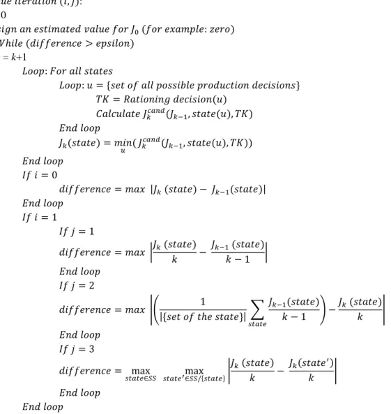
under the average system cost criterion using this formulation. The rationale behind this decision is twofold: i. Under the average cost criterion all the states converge to the same long-run average cost. However, the long-run discounted cost is state dependent and for such cases it is difficult to compare and interpret the performances of different policies. ii. We would like to exclude the discussion/decision about the determination of the discount rate 𝛼 and directly focus on the impacts of the real system parameters. However, we utilize the modified version of the discounted DP formulation given in Equation (1) to calculate the average system cost using the value iteration algorithm. To find the average cost, we set the discount rate to zero and at each stage divide the value of the cost-to-go function to the completed number of stages (otherwise the cost-to-go function would not converge to the finite average value) in the algorithm. Afterwards, we propose three different termination criteria for the value iteration:
1. The maximum of the absolute values of the difference between the average costs of two consecutive steps for all states is smaller than epsilon (a small number representing the tolerance for termination),
2. For each state, the maximum of the absolute value of the difference between the averages of the all state costs at the current step and all state costs at the previous step is smaller than epsilon,
3. For any step, the absolute value of the difference between the average costs of all states is smaller than epsilon,
When we use one of these termination conditions, the system cost can become finite. Either one of the above criteria can be utilized but we have decided to use the final one. The third one is the most reliable algorithm that checks the differences of the average costs for all the states. Using the first and second algorithms is risky, because the algorithm can be terminated before the all states converge to the same average cost. Pseudo-code of three value iteration algorithms is given in the following where k is for the current stage/step, 𝑖 represents whether we use the discounted cost criterion (𝑖 = 0) or the average (𝑖 = 1), and 𝑗 is the input for the above three termination criteria when 𝑖 = 1:
16 𝑉𝑎𝑙𝑢𝑒 𝑖𝑡𝑒𝑟𝑎𝑡𝑖𝑜𝑛 (𝑖, 𝑗): k = 0 𝐴𝑠𝑠𝑖𝑔𝑛 𝑎𝑛 𝑒𝑠𝑡𝑖𝑚𝑎𝑡𝑒𝑑 𝑣𝑎𝑙𝑢𝑒 𝑓𝑜𝑟 𝐽0 (𝑓𝑜𝑟 𝑒𝑥𝑎𝑚𝑝𝑙𝑒: 𝑧𝑒𝑟𝑜) 𝑊ℎ𝑖𝑙𝑒 (𝑑𝑖𝑓𝑓𝑒𝑟𝑒𝑛𝑐𝑒 > 𝑒𝑝𝑠𝑖𝑙𝑜𝑛) k = k+1 𝐿𝑜𝑜𝑝: 𝐹𝑜𝑟 𝑎𝑙𝑙 𝑠𝑡𝑎𝑡𝑒𝑠 𝐿𝑜𝑜𝑝: 𝑢 = {𝑠𝑒𝑡 𝑜𝑓 𝑎𝑙𝑙 𝑝𝑜𝑠𝑠𝑖𝑏𝑙𝑒 𝑝𝑟𝑜𝑑𝑢𝑐𝑡𝑖𝑜𝑛 𝑑𝑒𝑐𝑖𝑠𝑖𝑜𝑛𝑠} 𝑇𝐾 = 𝑅𝑎𝑡𝑖𝑜𝑛𝑖𝑛𝑔 𝑑𝑒𝑐𝑖𝑠𝑖𝑜𝑛(𝑢) 𝐶𝑎𝑙𝑐𝑢𝑙𝑎𝑡𝑒 𝐽𝑘𝑐𝑎𝑛𝑑(𝐽𝑘−1, 𝑠𝑡𝑎𝑡𝑒(𝑢), 𝑇𝐾) 𝐸𝑛𝑑 𝑙𝑜𝑜𝑝 𝐽𝑘(𝑠𝑡𝑎𝑡𝑒) = 𝑚𝑖𝑛𝑢 ( 𝐽𝑘𝑐𝑎𝑛𝑑(𝐽𝑘−1, 𝑠𝑡𝑎𝑡𝑒(𝑢), 𝑇𝐾)) 𝐸𝑛𝑑 𝑙𝑜𝑜𝑝 𝐼𝑓 𝑖 = 0 𝑑𝑖𝑓𝑓𝑒𝑟𝑒𝑛𝑐𝑒 = 𝑚𝑎𝑥 |𝐽𝑘 (𝑠𝑡𝑎𝑡𝑒) − 𝐽𝑘−1(𝑠𝑡𝑎𝑡𝑒)| 𝐸𝑛𝑑 𝑙𝑜𝑜𝑝 𝐼𝑓 𝑖 = 1 𝐼𝑓 𝑗 = 1 𝑑𝑖𝑓𝑓𝑒𝑟𝑒𝑛𝑐𝑒 = 𝑚𝑎𝑥 |𝐽𝑘 (𝑠𝑡𝑎𝑡𝑒) 𝑘 − 𝐽𝑘−1 (𝑠𝑡𝑎𝑡𝑒) 𝑘 − 1 | 𝐸𝑛𝑑 𝑙𝑜𝑜𝑝 𝐼𝑓 𝑗 = 2 𝑑𝑖𝑓𝑓𝑒𝑟𝑒𝑛𝑐𝑒 = 𝑚𝑎𝑥 |( 1 |{𝑠𝑒𝑡 𝑜𝑓 𝑡ℎ𝑒 𝑠𝑡𝑎𝑡𝑒}| ∑ 𝐽𝑘−1(𝑠𝑡𝑎𝑡𝑒) 𝑘 − 1 𝑠𝑡𝑎𝑡𝑒 ) −𝐽𝑘 (𝑠𝑡𝑎𝑡𝑒) 𝑘 | 𝐸𝑛𝑑 𝑙𝑜𝑜𝑝 𝐼𝑓 𝑗 = 3 𝑑𝑖𝑓𝑓𝑒𝑟𝑒𝑛𝑐𝑒 = max 𝑠𝑡𝑎𝑡𝑒∈𝑆𝑆 𝑠𝑡𝑎𝑡𝑒′max∈𝑆𝑆/{𝑠𝑡𝑎𝑡𝑒}| 𝐽𝑘 (𝑠𝑡𝑎𝑡𝑒) 𝑘 − 𝐽𝑘(𝑠𝑡𝑎𝑡𝑒′) 𝑘 | 𝐸𝑛𝑑 𝑙𝑜𝑜𝑝 𝐸𝑛𝑑 𝑙𝑜𝑜𝑝
Figure 3.1 The Pseudo-code of Value Iteration Algorithms
Our value iteration algorithm is verified with Ha (1997a) and Bulut and Fadıloğlu (2011) in the literature. The optimal production and rationing decisions mentioned in their studies are checked with our results. Besides these studies, it is known that the optimal policy is two-critical number policy (𝑋∗∗, 𝑋∗) for the
exponential systems include the setup cost. For such a system, we decide to start the numerical analysis with the setting (𝐾, 𝑠, 𝜇, ℎ, 𝜆1, 𝜆2, 𝑐1, 𝑐2) = (2, 1, 3, 1, 3, 1, 4,
17
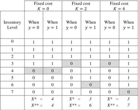
Table 3.1 Optimal Production Decisions up when s=1
Fixed cost
𝐾 = 0 Fixed cost 𝐾 = 2 Fixed cost 𝐾 = 4
Inventory Level When 𝑦 = 0 When 𝑦 = 1 When y = 0 When 𝑦 = 1 When 𝑦 = 0 When 𝑦 = 1 0 1 1 1 1 1 1 1 1 1 1 1 1 1 2 1 1 1 1 1 1 3 1 1 0 1 0 1 4 0 0 0 1 0 1 5 0 0 0 1 0 1 6 0 0 0 0 0 1 7 0 0 0 0 0 0 X* = 4 X** = 4 X* = 3 X** = 6 X* = 3 X** = 7
Table 3.1 shows the optimal production decisions when production is on (𝑠 = 𝑦 = 1) and off (𝑦 = 0). If there is no fixed cost to activate a new channel, the optimal production policy behaves like Base-Stock (𝑋∗= 𝑋∗∗ = 𝑆 = 4). While the
setup cost is a positive value, the system tries to extend the production process not to give extra cost to activate a channel again. There is a widening gap between the production control parameters while 𝐾 increases. According to the results of the table, we have similar optimal production policy properties mentioned in the literature.
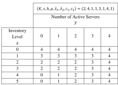
In the remaining part of this section and in the following sections, the parametric observations are analyzed and how the system parameters affect to the optimal decisions are shown using the base setting: (𝐾, 𝑠, ℎ, 𝜇, 𝜆1, 𝜆2, 𝑐1, 𝑐2) = (2, 4, 1, 1, 3, 1, 4, 1). The holding cost (ℎ = 1), the production rate (𝜇 = 1), demand rates of customer classes (𝜆1 = 3, 𝜆2 = 1) and the lost sales cost of these classes (𝑐1 = 4, 𝑐2 = 1) are determined. The optimal decisions for this system are shown in Table 3.2. Each row shows the inventory level and each row shows the number of active channels. For example, the first cell of the first row shows that the inventory
18
levels equals to zero (𝑥 = 0) and the production is off (𝑦 = 0). The value in the each cell of the decision matrix illustrates the number of servers is needed to be active.
Table 3.2 Optimal Production Decisions up
(𝐾, 𝑠, ℎ, 𝜇, 𝜆1, 𝜆2, 𝑐1, 𝑐2) = (2, 4, 1, 1, 3, 1, 4, 1)
Number of Active Servers 𝑦 Inventory Level 𝑥 0 1 2 3 4 0 4 4 4 4 4 1 3 3 3 3 4 2 2 2 2 3 4 3 2 2 2 3 4 4 0 1 2 3 4 5 0 1 2 3 4
If there is no active server and no inventory on-hand, the production decision is to use all of the limited capacity 𝑢𝑝(𝑥 = 0, 𝑦 = 0) = 4. While the number of active servers is fixed and the inventory level is increasing one by one, the optimal production decisions decrease by one or more units. That means, there is no constant order-up-to level. Instead, the target inventory of any state is state dependent. There is an order-up-to level for each inventory level 𝑆𝑥 = 𝑥 + 𝑢𝑝∗(𝑥, 0). Because, the system
does not want to give extra holding and setup cost by activating more channels.
For positive values of active servers, the cancellation cost of the production equals to infinity, so the production decisions decrease to at least the number of current active servers. For instance, when 𝑦 = 1 and while the inventory level is increasing, the optimal decision cannot be lower than 1 because no-order cancellation. Thus, the system controls the production by deciding the trade-off between holding and lost sales costs.
19
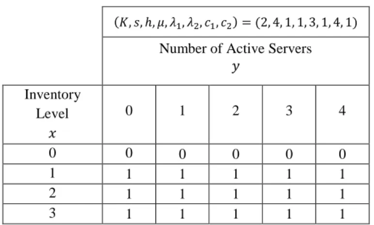
Table 3.3 Optimal Inventory Rationing Policy for Class 1
(𝐾, 𝑠, ℎ, 𝜇, 𝜆1, 𝜆2, 𝑐1, 𝑐2) = (2, 4, 1, 1, 3, 1, 4, 1)
Number of Active Servers 𝑦 Inventory Level 𝑥 0 1 2 3 4 0 0 0 0 0 0 1 1 1 1 1 1 2 1 1 1 1 1 3 1 1 1 1 1
Table 3.4 Optimal Inventory Rationing Policy for Class 2
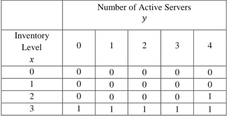
(𝐾, 𝑠, ℎ, 𝜇, 𝜆1, 𝜆2, 𝑐1, 𝑐2) = (2, 4, 1, 1, 3, 1, 4, 1)
Number of Active Servers 𝑦 Inventory Level 𝑥 0 1 2 3 4 0 0 0 0 0 0 1 0 0 0 0 0 2 0 0 0 0 1 3 1 1 1 1 1
Table 3.3 and 3.4 show the optimal rationing decisions for the customer class 1 and 2, respectively. In Table 3.3, if there is inventory on-hand, the system always satisfies an arriving demand of class 1. Because, the customer class 1 has the highest lost sales cost and is the most valuable class in the system. Table 3.4 shows that as inventory level and number of active servers increase, the willingness to satisfy a class 2 demand also increases. Hence, threshold inventory level for class 2 is a function of 𝑥 and 𝑦. Therefore, the inventory rationing policy is provided for just class 2.
Stock rationing gains importance when there are more than one demand class and each of them has different lost sales cost. If the lost sales costs of the classes are the same, the customer of the system becomes just a one class. When the lost sales costs are different, the production and rationing decisions are made jointly.
20
Table 3.5 and 3.6 show the optimal production and rationing decisions under the discounted cost criterion. For this example, the discount rate (𝛼) equals to 0.4. Even if the decisions in Table 3.2 and 3.5 are not the same, the characteristics of the production policies are not so different. This situation is also valid for stock rationing decisions.
Table 3.5.Optimal Production Decisions Under Discounted Cost Criterion
Number of Active Servers 𝑦 Inventory Level 𝑥 0 1 2 3 4 0 3 3 3 3 4 1 2 2 2 3 4 2 1 1 2 3 4 3 0 1 2 3 4 4 0 1 2 3 4 5 0 1 2 3 4
Table 3.6 Optimal Rationing Decisions Under Discounted Cost Criterion
Number of Active Servers 𝑦 Inventory Level 𝑥 0 1 2 3 4 0 0 0 0 0 0 1 0 0 0 0 0 2 0 0 0 0 1 3 1 1 1 1 1
3.3 The Impact of the System Parameters on the Optimal Policies
This section includes the analysis of how the system parameters affect the optimal policies of 𝑀/𝑀/𝑠 make-to-stock queues with fixed cost. The most important parameters for such a system are the fixed cost (𝐾) and number of available servers (𝑠). First of all, the impacts of the fixed cost and number of servers on optimal production and rationing decisions are analyzed, and then the impacts of the other parameters are shown in the following sections.
21
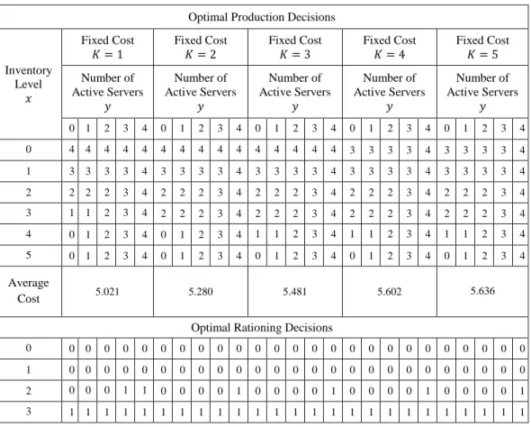
Table 3.7 The Impact of the Fixed Cost on Optimal Decisions
Optimal Production Decisions
Inventory Level
𝑥
Fixed Cost
𝐾 = 1 Fixed Cost 𝐾 = 2 Fixed Cost 𝐾 = 3 Fixed Cost 𝐾 = 4 Fixed Cost 𝐾 = 5 Number of Active Servers 𝑦 Number of Active Servers 𝑦 Number of Active Servers 𝑦 Number of Active Servers 𝑦 Number of Active Servers 𝑦 0 1 2 3 4 0 1 2 3 4 0 1 2 3 4 0 1 2 3 4 0 1 2 3 4 0 4 4 4 4 4 4 4 4 4 4 4 4 4 4 4 3 3 3 3 4 3 3 3 3 4 1 3 3 3 3 4 3 3 3 3 4 3 3 3 3 4 3 3 3 3 4 3 3 3 3 4 2 2 2 2 3 4 2 2 2 3 4 2 2 2 3 4 2 2 2 3 4 2 2 2 3 4 3 1 1 2 3 4 2 2 2 3 4 2 2 2 3 4 2 2 2 3 4 2 2 2 3 4 4 0 1 2 3 4 0 1 2 3 4 1 1 2 3 4 1 1 2 3 4 1 1 2 3 4 5 0 1 2 3 4 0 1 2 3 4 0 1 2 3 4 0 1 2 3 4 0 1 2 3 4 Average Cost 5.021 5.280 5.481 5.602 5.636
Optimal Rationing Decisions
0 0 0 0 0 0 0 0 0 0 0 0 0 0 0 0 0 0 0 0 0 0 0 0 0 0 1 0 0 0 0 0 0 0 0 0 0 0 0 0 0 0 0 0 0 0 0 0 0 0 0 0 2 0 0 0 1 1 0 0 0 0 1 0 0 0 0 1 0 0 0 0 1 0 0 0 0 1 3 1 1 1 1 1 1 1 1 1 1 1 1 1 1 1 1 1 1 1 1 1 1 1 1 1
In Table 3.7, when there is a small fixed cost to activate a new channel, the system operates with more channels than when there is a larger fixed cost to activate a new one. Because, the system chooses to pay the lost sales cost instead of paying the fixed cost. As 𝐾 increases, the production continues not to give setup cost more than one, even if inventory level is higher. For example, when 𝐾 = 4 and (𝑥, 𝑦) = (4,0) the optimal production decision is to continue to production with one active server. However, when 𝐾 = 1 and (𝑥, 𝑦) = (4,0) the optimal decision equals to zero. Also, the average cost increases as 𝐾 increases.
The impact of the fixed cost on optimal rationing policy is not very significant for this example. Because, the demand rate of class 2 is very low. If the demand rate increases, the effect of the fixed cost can be observed. For this example, the rationing decision for class 2 demand is expressed as 𝑢𝑟 such that 𝑢𝑟 ∈ {0,1}. If 𝑢𝑟 = 1, class 2 demand is satisfied; else, it is rejected. When 𝐾 = 1 and (𝑥, 𝑦) = (2,3) the optimal
22
rationing decision is to satisfy the arriving class 2 demand. However, when 𝐾 > 1 and (𝑥, 𝑦) = (2,3) the decision is not to reject the arriving class 2 demand. When there is a high fixed cost to activate a new channel, the system satisfies the demand in higher inventory position.
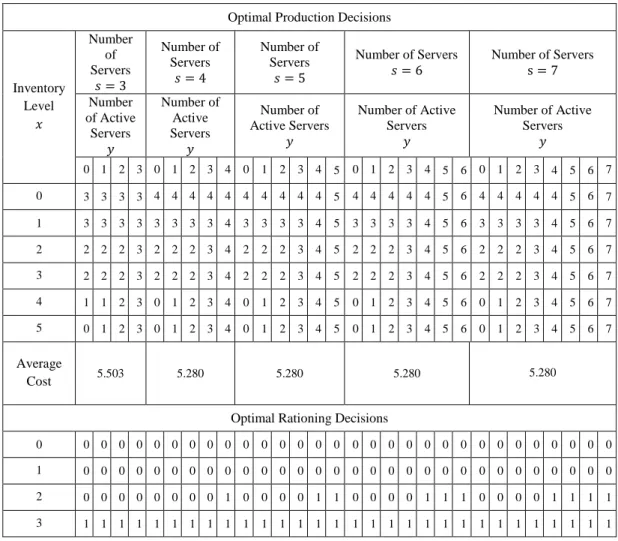
Table 3.8 The Impact of Number of Servers on Optimal Decisions
Optimal Production Decisions
Inventory Level 𝑥 Number of Servers 𝑠 = 3 Number of Servers 𝑠 = 4 Number of Servers 𝑠 = 5 Number of Servers 𝑠 = 6 Number of Servers s = 7 Number of Active Servers 𝑦 Number of Active Servers 𝑦 Number of Active Servers 𝑦 Number of Active Servers 𝑦 Number of Active Servers 𝑦 0 1 2 3 0 1 2 3 4 0 1 2 3 4 5 0 1 2 3 4 5 6 0 1 2 3 4 5 6 7 0 3 3 3 3 4 4 4 4 4 4 4 4 4 4 5 4 4 4 4 4 5 6 4 4 4 4 4 5 6 7 1 3 3 3 3 3 3 3 3 4 3 3 3 3 4 5 3 3 3 3 4 5 6 3 3 3 3 4 5 6 7 2 2 2 2 3 2 2 2 3 4 2 2 2 3 4 5 2 2 2 3 4 5 6 2 2 2 3 4 5 6 7 3 2 2 2 3 2 2 2 3 4 2 2 2 3 4 5 2 2 2 3 4 5 6 2 2 2 3 4 5 6 7 4 1 1 2 3 0 1 2 3 4 0 1 2 3 4 5 0 1 2 3 4 5 6 0 1 2 3 4 5 6 7 5 0 1 2 3 0 1 2 3 4 0 1 2 3 4 5 0 1 2 3 4 5 6 0 1 2 3 4 5 6 7 Average Cost 5.503 5.280 5.280 5.280 5.280
Optimal Rationing Decisions
0 0 0 0 0 0 0 0 0 0 0 0 0 0 0 0 0 0 0 0 0 0 0 0 0 0 0 0 0 0 0 1 0 0 0 0 0 0 0 0 0 0 0 0 0 0 0 0 0 0 0 0 0 0 0 0 0 0 0 0 0 0 2 0 0 0 0 0 0 0 0 1 0 0 0 0 1 1 0 0 0 0 1 1 1 0 0 0 0 1 1 1 1 3 1 1 1 1 1 1 1 1 1 1 1 1 1 1 1 1 1 1 1 1 1 1 1 1 1 1 1 1 1 1
Table 3.8 shows the effect of number of servers on optimal decisions. If available processing channels are scarce (𝑠 = 3), the optimal production policy tries to use all of the limited capacity. When 𝑠 > 4, the system is equivalent to a system with uncapacitated replenishment channel, because it always activates less than the available 𝑠 channels and therefore additional channels do not provide further gain. Also, the average costs do not change because there is no difference in production decisions after 𝑠 = 4.
23
If available processing channels are scarce (𝑠 = 3), the system satisfies an arriving class 2 demand in high inventory levels. As number of available servers increases, the system also reserves the inventory for class 2 demand. Because, if more inventory is needed, it can be replenished in a short time by using all limited capacity. Like production decisions after 𝑠 = 4 there is no difference in rationing decisions.
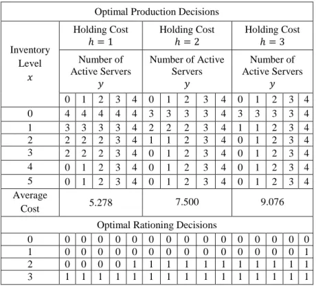
Table 3.9 The Impact of Holding Cost on Optimal Decisions
Optimal Production Decisions
Inventory Level 𝑥 Holding Cost ℎ = 1 Holding Cost ℎ = 2 Holding Cost ℎ = 3 Number of Active Servers 𝑦 Number of Active Servers 𝑦 Number of Active Servers 𝑦 0 1 2 3 4 0 1 2 3 4 0 1 2 3 4 0 4 4 4 4 4 3 3 3 3 4 3 3 3 3 4 1 3 3 3 3 4 2 2 2 3 4 1 1 2 3 4 2 2 2 2 3 4 1 1 2 3 4 0 1 2 3 4 3 2 2 2 3 4 0 1 2 3 4 0 1 2 3 4 4 0 1 2 3 4 0 1 2 3 4 0 1 2 3 4 5 0 1 2 3 4 0 1 2 3 4 0 1 2 3 4 Average Cost 5.278 7.500 9.076
Optimal Rationing Decisions
0 0 0 0 0 0 0 0 0 0 0 0 0 0 0 0
1 0 0 0 0 0 0 0 0 0 0 0 0 0 0 1
2 0 0 0 0 1 1 1 1 1 1 1 1 1 1 1
3 1 1 1 1 1 1 1 1 1 1 1 1 1 1 1
In Table 3.9, as the holding cost increases, the system operates with fewer channels. Because, the system does not prefer to stock not to give extra holding cost. This decision should be made by evaluating the balance of the holding and lost sales cost. While the holding cost increases, the average cost increases unsurprisingly.
When ℎ = 1, an arriving demand class 2 is satisfied if the inventory level equals 3 or (𝑥, 𝑦) = (2,4). As the holding cost increases, the threshold level decreases and the system starts to satisfy an arriving class 2 demand in lower inventory levels.
24
Table 3.10 The Impact of Production Rate on Optimal Decisions
Optimal Production Decisions Inventory
Level 𝑥
Production Rate
𝜇 = 1 Production Rate 𝜇 = 2 Production Rate 𝜇 = 3 Number of Active Servers 𝑦 Number of Active Servers 𝑦 Number of Active Servers 𝑦 0 1 2 3 4 0 1 2 3 4 0 1 2 3 4 0 4 4 4 4 4 2 2 2 3 4 2 2 2 3 4 1 3 3 3 3 4 2 2 2 3 4 1 1 2 3 4 2 2 2 2 3 4 1 1 2 3 4 1 1 2 3 4 3 2 2 2 3 4 1 1 2 3 4 0 1 2 3 4 4 0 1 2 3 4 0 1 2 3 4 0 1 2 3 4 5 0 1 2 3 4 0 1 2 3 4 0 1 2 3 4 Average Cost 5.280 5.044 4.837
Optimal Rationing Decisions
0 0 0 0 0 0 0 0 0 0 0 0 0 0 0 0
1 0 0 0 0 0 0 0 0 0 1 0 0 0 1 1
2 0 0 0 0 1 0 0 1 1 1 1 1 1 1 1
3 1 1 1 1 1 1 1 1 1 1 1 1 1 1 1
Table 3.10 shows the effect of increasing the production rate on optimal decisions and the average cost. As the production rate increases, the system does not activate all of the limited capacity. If the production rate is high, the processing time takes a short time. Hence, the system activates fewer channels. For example, when the production rate is small (𝜇 = 1), the system is willing to operate with all available channels. However when 𝜇 = 3, the system does not need to activate all channels. Thus, the system activates more channels when the production rate is low otherwise; the system activates fewer channels when the production rate is high. To activate more channels when there is high production rate causes to increasing the average cost because of the fixed and holding costs.
When the production rate is low, an arriving class 2 demand is satisfied in higher inventory levels. The system wants to reserve the inventory in anticipation of future demand from class 1. However, the production rate is high (𝜇 = 3) the system starts to satisfy class 2 demand is fewer inventory levels. Because of low production time the production is completed in a short time and arriving class 1 demand can be also satisfied in a short time.
25
Table 3.11 The Impact of Demand Rates on Optimal Decisions
Optimal Production Decisions
Inventory Level
𝑥
Demand rate
𝜆1= 3, 𝜆2= 1 𝜆1Demand rate = 2.5, 𝜆2= 1.5 𝜆Demand rate 1= 2, 𝜆2= 2 𝜆1Demand rate = 1.5, 𝜆2= 2.5 𝜆Demand rate 1= 1, 𝜆2= 3
Number of Active Servers 𝑦 Number of Active Servers 𝑦 Number of Active Servers 𝑦 Number of Active Servers 𝑦 Number of Active Servers 𝑦 0 1 2 3 4 0 1 2 3 4 0 1 2 3 4 0 1 2 3 4 0 1 2 3 4 0 4 4 4 4 4 4 4 4 4 4 3 3 3 3 4 3 3 3 3 4 3 3 3 3 4 1 3 3 3 3 4 3 3 3 3 4 3 3 3 3 4 2 2 2 3 4 2 2 2 3 4 2 2 2 2 3 4 2 2 2 3 4 2 2 2 3 4 2 2 2 3 4 1 1 2 3 4 3 2 2 2 3 4 1 1 2 3 4 1 1 2 3 4 1 1 2 3 4 0 1 2 3 4 4 0 1 2 3 4 0 1 2 3 4 0 1 2 3 4 0 1 2 3 4 0 1 2 3 4 5 0 1 2 3 4 0 1 2 3 4 0 1 2 3 4 0 1 2 3 4 0 1 2 3 4 Average Cost 5.280 5.007 4.680 4.359 4.112
Optimal Rationing Decisions
0 0 0 0 0 0 0 0 0 0 0 0 0 0 0 0 0 0 0 0 0 0 0 0 0 0 1 0 0 0 0 0 0 0 0 0 0 0 0 0 0 0 0 0 0 0 0 0 0 0 1 1 2 0 0 0 0 1 0 0 0 1 1 1 1 1 1 1 1 1 1 1 1 1 1 1 1 1 3 1 1 1 1 1 1 1 1 1 1 1 1 1 1 1 1 1 1 1 1 1 1 1 1 1
In Table 3.11, when class 1 demand rate is higher than class 2 demand rate, the system tries to produce with more servers. Because, class 1 is the most valuable demand class and its demand occur in a short time. Hence, the system desires to satisfy class 1 demand by activating more production channels (𝜆1 = 3, 𝜆2 = 1). If
the system activates fewer channels, it may pay the lost sales cost. As class1 demand rate decreases and class 2 demand rate increases, the balance changes. Because, the amount of class 1 demand is less than the amount of class 2 demand in a unit time (𝜆1 = 1, 𝜆2 = 3). Hence, the system does not activate all of the limited capacity
because of a low demand of the most valuable class.
When the class 1 demand rate is high, class 2 demand is satisfied while increasing of inventory level and number of active channels. As the class 2 demand rate exceeds the demand rate of class 1, the rationing level decreases. The system starts to satisfy less valuable demand class in low inventory levels.
26
Table 3.12 The Impact of Lost Sales Costs on Optimal Decisions
Optimal Production Decisions Inventory
Level 𝑥
Lost sales cost 𝑐1= 3, 𝑐2= 1
Lost sales cost 𝑐1= 4, 𝑐2= 1
Lost sales cost 𝑐1= 5, 𝑐2= 1 Number of Active Servers 𝑦 Number of Active Servers 𝑦 Number of Active Servers 𝑦 0 1 2 3 4 0 1 2 3 4 0 1 2 3 4 0 3 3 3 3 4 4 4 4 4 4 4 4 4 4 4 1 3 3 3 3 4 3 3 3 3 4 3 3 3 3 4 2 3 3 3 3 4 2 2 2 3 4 3 3 3 3 4 3 1 1 2 3 4 2 2 2 3 4 2 2 2 3 4 4 0 1 2 3 4 0 1 2 3 4 1 1 2 3 4 5 0 1 2 3 4 0 1 2 3 4 0 1 2 3 4 Average Cost 4.862 5.280 5.664
Optimal Rationing Decisions
0 0 0 0 0 0 0 0 0 0 0 0 0 0 0 0
1 0 0 0 0 0 0 0 0 0 0 0 0 0 0 0
2 1 1 1 1 1 0 0 0 0 1 0 0 0 0 0
3 1 1 1 1 1 1 1 1 1 1 1 1 1 1 1
Table 3.12 exhibits the effect of lost sales cost of class 1 on optimal production and rationing decisions. If the lost sales cost of class 1 is small, the optimal production decisions are less than the others. Even if the system cannot satisfy the demand of class 1, the lost sales cost will be paid is small (𝑐1 = 3, 𝑐2 = 1). However, as the lost sales cost increases, the system starts to use all of the available servers in order to increase average inventory level and not to pay high lost sales cost per item (𝑐1 = 5, 𝑐2 = 1). As the lost sales cost increases, the average cost increases as well.
While the lost sales cost of class 1 is close to the lost sales cost of class 2, the system satisfies an arriving class 2 demand in low inventory levels but as the difference of the lost sales cost increases, the system starts to reserve inventory for more valuable demand class in order not to pay the lost sales cost of class 1.
Based on above numerical observations the detailed characterization of optimal production and rationing polices can be provided with the following conjectures. For a given state (𝑥, 𝑦), if the number of active channels is less than or equal to the optimal number of active channels at state (𝑥, 0), the production decision equals to
27
𝑢𝑝∗(𝑥, 0); else the production decision is not to change the number of active channels
(𝑖). i. 𝑢𝑝∗(𝑥, 𝑦) = { 𝑢𝑝∗(𝑥, 0) , 𝑦 ≤ 𝑢 𝑝 ∗(𝑥, 0) 𝑦 , 𝑦 > 𝑢𝑝∗(𝑥, 0)
The optimal number of active channels at state (𝑥, 0) decreases by one or more units for each unit increase in the on-hand inventory level and then it remains constant at zero. It is non-increasing in inventory on hand (ii). There are different order-up-to levels for each inventory level (iii). The optimal number of production channels is non-increasing in the inventory level (iv).
ii. 𝑢𝑝∗(𝑥, 0) − 𝑢𝑝∗(𝑥 + 1,0) ≥ 1 .
iii. 𝑆𝑥= 𝑥 + 𝑢𝑝∗(𝑥, 0), ∀𝑥.
iv. 𝑢𝑝∗(𝑥, 𝑦) ≥ 𝑢𝑝∗(𝑥 + 𝑘, 𝑦), ∀𝑥, 𝑦, 𝑘 ≥ 1.
The effects of the system parameters which are fixed cost (𝐾), holding cost (ℎ), production rate (𝜇) and traffic rates (𝜆1, 𝜆2) on optimal production and
rationing policies are shown as the following. 𝑢𝑝∗(𝑥, 𝑦) and 𝑢𝑟∗𝑗(𝑥, 𝑦) are expressed as optimal production and rationing decisions, respectively (v, vi, vii, viii).
v. 𝑢𝑝,𝐾1 ∗ (𝑥, 𝑦) ≥ 𝑢 𝑝,𝐾2 ∗ (𝑥, 𝑦) 𝑎𝑛𝑑 𝑢 𝑟𝑗,𝐾1 ∗ (𝑥) ≥ 𝑢 𝑟𝑗,𝐾2 ∗ (𝑥) , ∀𝑥 𝑎𝑛𝑑 𝑦, 𝐾1 ≤ 𝐾2, 𝑗 = 1,2. vi. 𝑢𝑝,ℎ∗ 1(𝑥, 𝑦) ≥ 𝑢𝑝,ℎ∗ 2(𝑥, 𝑦) 𝑎𝑛𝑑 𝑢𝑟∗𝑗,ℎ1(𝑥) ≤ 𝑢𝑟∗𝑗,ℎ2(𝑥) , ∀𝑥 𝑎𝑛𝑑 𝑦, ℎ1 ≤ ℎ2, 𝑗 = 1,2. vii. 𝑢𝑝,𝜇∗ 1(𝑥, 𝑦) ≥ 𝑢𝑝,𝜇∗ 2(𝑥, 𝑦) 𝑎𝑛𝑑 𝑢∗𝑟𝑗,𝜇1(𝑥) ≤ 𝑢𝑟∗𝑗,𝜇2(𝑥) , ∀𝑥 𝑎𝑛𝑑 𝑦, 𝜇1 ≤ 𝜇2, 𝑗 = 1,2. viii. 𝑢𝑝,𝜆1 ∗ (𝑥, 𝑦) ≤ 𝑢 𝑝,𝜆2 ∗ (𝑥, 𝑦) , ∀𝑥 𝑎𝑛𝑑 𝑦, 𝜆 1 ≤ 𝜆2.
ix. There exists a threshold inventory level 𝑅𝑥𝑖(𝑦) for demand class 𝑖 ≥ 2, which
28
than 𝑅𝑥𝑖(𝑦), it is optimal to satisfy; else it should be rejected. 𝑅𝑥𝑁(𝑦) ≥ 𝑅𝑥𝑁−1(𝑦) ≥ ⋯ ≥ 𝑅𝑥2(𝑦) ≥ 0 and 𝑅𝑥𝑖(𝑦 + 1) ≤ 𝑅𝑥𝑖(𝑦) for 𝑖 ∈ {2, … , 𝑁}.
x. There exists a threshold number of active channels 𝑅𝑦𝑖(𝑥) for demand class 𝑖 ≥ 2, which is a function inventory level 𝑥. If the number of active production channels is more than 𝑅𝑦𝑖(𝑥), it is optimal to satisfy; else it should
be rejected. 𝑅𝑦𝑁(𝑥) ≥ 𝑅𝑦𝑁−1(𝑥) ≥ ⋯ ≥ 𝑅𝑦2(𝑥) ≥ 0 and 𝑅𝑦𝑖(𝑥 + 1) ≤ 𝑅𝑦𝑖(𝑥) for 𝑖 ∈ {2, … , 𝑁}.
29
4 THE PROPOSED PRODUCTION AND RATIONING POLICIES
According to the numerical observations of the optimal policies, optimal policies are highly dynamic and do not have systematic behaviour for practical purposes. It is not so easy to be applied in the firms. Hence, proposing new/alternative policies whose performances are close to performances of the optimal policy and have a general behaviour to be applied can be beneficial. In this section, the characteristics and behaviours of the alternative production and rationing policies are deeply analyzed.
The rest of this section is organized as follows. In Section 4.1, we introduce three different production policies and discuss the properties of these policies. The Sub-section 4.1.2.2 includes Continuous Time Markov Chain analysis to get the steady-state probabilities of the production policy 2. In Sub-section 4.1.3.3, a renewal analysis utilizing renewal reward theorem is conducted to calculate the average cost for production policy 3 when s = 1, which is the optimal policy for single-server case. Also, we compare the performances of the proposed policies with optimal and Base-stock policies in the literature.
4.1 The Proposed Production Policies
The performances of the proposed policies can be compared with the Base-stock and optimal policies. Base-Base-stock policy has only one critical level which is called as 𝑆. When inventory level drops to below 𝑆, the production is triggered and starts. In other words, the system turns to (𝑆, 𝑆 − 1). When inventory level hits to 𝑆 − 1, the production starts and continues until inventory level reaches to 𝑆. Base-stock policy is the optimal production policy for 𝑀/𝑀/1 make-to-stock queues with no fixed cost.
The optimal production policy for 𝑀/𝑀/1 make-to-stock queues with fixed cost is (𝑋∗, 𝑋∗∗). Base-stock policy is a special case of (𝑋∗, 𝑋∗∗) policy. If 𝑋∗∗ =