A Numerical Solution of the One Dimensional Groundwater Flow by Transfer Matrix Method

3 (2), 2009, 161 - 164

©BEYKENT UNIVERSITY

A Numerical Solution of the One Dimensional

Groundwater Flow by Transfer Matrix Method

Rasoul DANESFARAZ

and Birol KAYA

department of Civil Eng., University of Maragheh, Maragheh, Iran.

2Department of Civil Eng., University of Dokuz Eylül, Buca, Izmir, Turkey.

daneshfaraz@yahoo.com birol.kaya@deu.edu.tr

Received: 01.04.2009, Revised: 07.04.2009, Accepted: 13.07.2009

Abstract

Transfer matrix method is applied to one dimensional initial value problems. The use of this method in hydraulic engineering is not widespread and only limited studies are available. The method is applied to one dimensional groundwater flow problems for the first time. In this study, a new approach via transfer matrix method has been presented for the solution of one dimensional groundwater flow representing parabolic type partial differential equation. A confined aquifer of constant or varying boundary conditions is selected as on illustrative example. The problem was solved for heterogeneous soil. Finite element method, finite difference method and transfer matrix methods proposed in this study were utilized for numerical solution. The outcomes of the three methods are compared. Regarding to the outcomes of the transfer matrix method, it can be revealed that the model is quite easily programmable and the solution obtained is seldom divergent.

Keywords: Groundwater hydraulics, Transfer matrix, Confined aquifers, Unsteady flow, Parabolic differential equation.

Özet

Transfer matrisi yöntemi tek boyutlu akım problemlerine uygulanmıştır.Yöntemin hidrolik problemlerine uygulanması yaygın olmayıp bir kaç çalışmayla sınırlıdır. Yöntem tek boyutlu yeraltı suyu problemlerine bu çalışmayla ilk defa uygulanmıştır. Yöntem, tek boyutlu parabolik kısmi diferansiyel denklem içeren yeraltı suyu problemlerine uygulanmıştır Örneklerde Akifer için sabit veya değişken sınır koşulları dikkate alınmıştır.. Problem heterojen zeminler için uygulanmıtır. Çalışmanın sonunda yöntemin uygunluğunu göstermek üzere çözülen örneklerde Sonlu farklar ve sonlu elemanlar yöntemleri de karşılaştırma amacıyla kullanılmıştır.. Örneklerden yöntemin yeter uygunlukta sonuç verdiği gözlenmiştir.

Keywords: Yeraltı suyu hidroliği, Taşıma matrisi, Basınçlı aquifer, Kararsız akım, Parabolic denklemler.

1. Introduction

Investigating the studies related to the solution of groundwater flow in the literature, underlined that the transfer matrix methodology is applied to 1D groundwater flow problems for the first time. Some other related studies are as follows.

Developed analytical solutions based on the Laplace transform method in order to describe the rise and fall of the water table and the groundwater velocities in finite and semi-infinite stream-aquifer systems. Sinusoidal and asymmetric flood wave in the stream were considered to determine transient solutions[5]. Employed a similar approach, with a discrete number of time steps and a finite difference scheme of numerical integration, in order to solve several transient unconfined groundwater problems. The axisymmetric flow to a pumping well and the free surface behavior within a dam when the reservoir water level is suddenly lowered, were determined with isoparametric elements in the prior case and linear approximated elements in the latter case, for different times[16]. Investigated a one-dimensional groundwater transport equation with two uncertain parameters, groundwater velocity and longitudinal dispersivity. They used Monte Carlo simulation to investigate the uncertainty of one-dimensional groundwater flow field in non-uniform homogeneous media[12]. Used the perturbation approach to analyze the groundwater flow field by taking the spatial variability of the hydraulic conductivity into consideration. Method of Taylor series expansion is more straightforward than the perturbation method[2]. Fatullayev and Can used, an inverse problem is formulated to determine water capacity of porous media. They used Finite Difference Method for solution of parabolic equation[8]. Koutitas (1982) solved nonlinear groundwater flows with the use of Finite Element and Finite difference methods.

Allen and Murphy presented a finite element collocation method for variably saturated flows in porous media[1].

Saenton et al. and Saenton developed an explicittly coupled finite difference mass transfer model based on existing groundwater flow program, MODFLOW[17,18].

Khebchareon and Saenton used Crank-Nicolson and Galerkin finite element methods for 1D groundwater[10]. Srivastava, Serrano and Workman used stochastic modeling of transient stream-aquifer interaction with the nonlinear Boussinesq equation. They offered analytical solution for nonlinear Boussinesq equation[20].

Time dependent parabolic equations are representative models of unsteady flows in nature. These equations have main importance in engineering. The equations explaining the 1D groundwater flow are parabolic partial differential. The transfer matrix method utilized in this study is not widely known in hydraulic engineering. In transfer matrix method, which is also known as the method of initial values where, the aim is to convert problem of boundary values into problem of initial value prevent new constant values and to express equations of the problem by initial constant values. With the help of this method, many problems in hydraulics can be solved. Limited applications in the literature are listed below.

Baume, Sau and Malaterre expressed a need for using linear control theory while pointing out the difficulty of complex hydraulic systems to control. They obtained a reach transfer matrix by liberation of Saint Venant equations near a steady flow regime. In this study Saint Venant equations were used in an hydraulic application for the first time. However, the equations were used between two given points only[3].

Litrico and Flomionused Transfer matrix method to obtain a frequency domain model of Saint-Venant equations, linearized around any stationary regime, including backwater curves[13,14].

Litrico and Flomioninvestigated the control of oscillating modes occurring in open channels, due to the reflection of propagating waves on the boundaries. They characterized the effect of a proportional boundary control on the poles of the transfer matrix by a root locus which derived to an asymptotic result for high frequencies closed loop poles[15].

Chaudry used Transfer Matrix Method for waterhammer calculation in neglecting v.dv/dx in dynamic equation[4].

Shimada et al. introduced an exact method of assessing numerical errors in analyses of unsteady flows in pipe networks. A pipe polynomial transfer matrix had been developed and was analogous to transfer function matrices used in free oscillation theory[19].

Daneshfaraz and Kaya have applied the transfer matrix method to 1D pipe hydraulic problems. The authors have applied the method on two problems and compared the solutions with FE method. They have also emphasized that the method is easily programmable and stable[6].

Daneshfaraz and Kaya have used Transfer Matrix method for waves propagation in open channel flow[7].

2. Groundwater Flow Equations

The basic equations of groundwater flow are obtained by means of mass and energy conservation principles combined with Darcy law [9].

Altering flow and soil properties in three directions in space, namely x, y, z; and in the case of unsteady flow, the change in mass by time is:

àqx +

y + dq

dx dy dz

S

dh

(1)

b

dt

In this equation, x, y and z are coordinates, t is time, S is the storage coefficient, b is the aquifer thickness, h is the piesometric height, qx, qy and qz are the unit discharge values in x, y and z directions, respectively. kx, ky and kz are permeability coefficients in three directions. Using Darcy's law the following equations can be written.

,

dh

qx

=

x y ( 2 )

dx

, dh

y =

y

dy

dh

q

z

=

dz

Assuming that the soil is homogeneous and isotropic (Kx=Ky= Kz =K); the flow

in a confined aquifer, the combination of Eqs 1, 2, 3 and 4 gives:

d

h d

h d

h

ô—+ ÎT + ÎT

dx

dy

dz

S dh

- • —

T

dt

In this equation T is the transmissivity capacity which is expressed as follows:

T=b.k (6a) In the heterogenous soil, the transmissivity capacity can be calculate as:

T=b1k1+b2k2+b3k3+ (6b) Equation (5); written for flow in 3D homogeneous and isotropic pore media is

d

h

dx 2

S

dh

T

'

dt

3. USE OF TRANSFER MATRIX METHODS

Different numerical methods can be used to solve parabolic equations. In this study, finite difference, finite element and transfer matrix methods were used. In finite difference solution, explicit approach is preferred. In finite element method, Galerkin method is applied with quadratic elements[21].

In engineering problems, the calculation procedure is laborious and prone to errors if the number of constants to be determined by boundary conditions is very high. Therefore, it is of main importance to keep the constants of integration at their minimum numbers. The transfer matrix method is very efficient in this procedure. In this method, which is applicable to 1D problems, it is aimed to transform the boundary value problems into initial value problems.

The use of transfer matrix method enables the user to find out the solution of many problems in a shorter time and an easier way, in comparison with other methods.

For a while, by neglecting the time variable term:

a

h

2

0

dx

The solution depending on x is obtained as follows;

dh

— = C

dx

h = Q x +

dh

From boundary conditions, we have C i = ( )Q and C 2 = h g .

dx

Substituting the constants and considering time derivative, the following equations can be written for node(i+1) at time step n:

A

dh r .

x + h

i+1

dx

dx

_i+1

Ji

'

dh

dx

_i

un un-1

i+1

i+1

Dt

S

— •Ax

T

The unknown values at point (i+1) may be found from

S Dx

,

n

(

dh

\

(

dh

i+1 +

T Dt

_{v dx}

_i+1

dx

h + 1

. £ .Dx

i

Dt T

Equations (11) and (13) can be written by using matrix form;

1

0

1

0 1

(

0

and finally, making the necessary arrangements Equation 15.1 can be obtained: (15.1) D x hi + 1 1 x " hn ' " 0 = + hT+l1 S (dh n (^ ~)i + 1 dx _ £ Dx £ Dx x + 1 ( d h ) n _ dx ' _ hT+l1 S (dh n (^ ~)i + 1 dx _ _ _T ' Â 7 T Dt _ ( d h ) n _ dx ' _ _ D t T

The transfer matrix of the system is

t

i

1

x

S Dx S Dx

x +1

T Dt T Dt

and F presents the time effect on node point the time-dependent values in addition node points

0

F + 1 =

hn+1

. S . Dx

Dt T

The equations (15.1), (15.2) and (15.3) can be rewritten as

f

+ 1

" f '

^n

+1

_ dx _

II

_t

n

i

_ dx _

+ F

_i+1

The indeterminates at initial and final points of the system equation are determined by boundary conditions. Afterwards, the indeterminates at other points are determined by using these values.

4. Numerical Examples

The interval between the nodes (Ax) is taken as 10m. In order to achieve a

TAt

convergent solution, value is ensured to be under 0.5. In this case,

S (Ax)

At should be selected below 5 minutes[21].

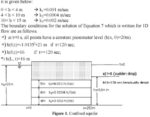
The pressure aquifer; which is given in Figure 1. has a storage coefficient(S) of 0.002 and length (L) of 250m. The aquifer has different k values that taken as it is given below:

0 < h < 4 m ^ k1=0.001 m/sec 4 < h < 10 m ^ k2=0.0004 m/sec

10< h < 15 m ^ k3=0.002 m/sec

The boundary conditions for the solution of Equation 7 which is written for 1D flow are as follows.

*) at t=0 s, all points have a constant piesometer level (h(x, 0)=20m).

*) h(0,t)=-1.0135t+21 m if t<120 sec;

*) h(0,t)=16 if t>= 120 sec; *) h(L, t)=16 m

x=0 x=25Iirri

Figure 1. Confined aquifer

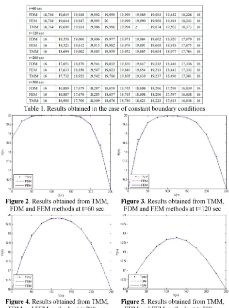
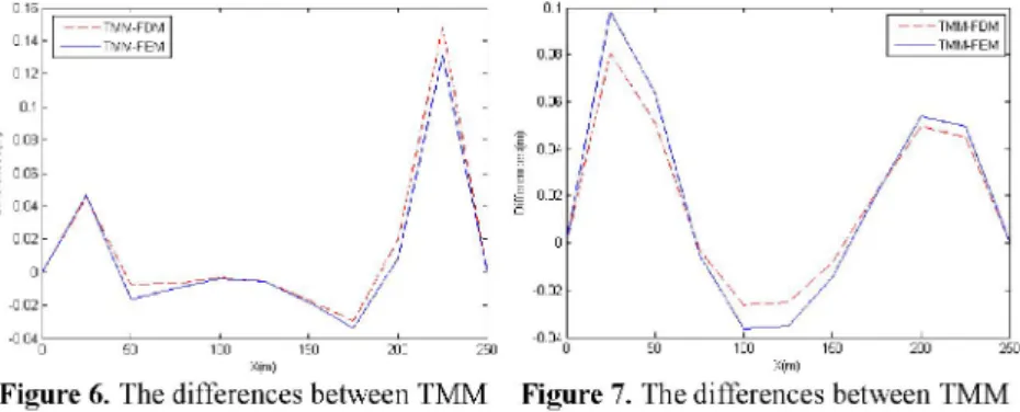
The water level changes are calculated using transfer matrix method (TMM); at t=60, t=120, t=200 and t=500 sec; which are compared with the finite element method (FEM) and finite difference method (FDM) solutions of Wang, Anderson(1995) for the same problem. The results are given in Table 1 and Figures 2, 3, 4 and 5. Differences between TMM and other methods are given Figures 6 and 7.

1=60 sec FDM 18,764 19,645 19,938 19,992 19,999 19,999 19,989 19,903 19,482 18,226 16 FEM 18,764 19,644 19,947 19,995 20 19,999 19,990 19,908 19,494 18,243 16 TMM 18,764 19,690 19,931 19,986 19,996 19,994 2 19,874 19,502 18,373 16 1=120 sec FDM 16 18,558 19,606 19,906 19,977 19,97! 19,884 19,602 18,920 17,679 16 FEM 16 18,521 19,612 19,915 19,982 19,976 19,891 19,608 18,919 17,675 16 TMM 16 18,694 19,602 19,883 19,959 19,952 19,865 19,604 18,977 17,764 16 1=200 sec FDM 16 17,651 18,870 19,544 19,812 19,830 19,647 19,212 18,446 17,336 16 FEM 16 17,633 18,858 19,547 19,823 19,840 19,654 19,213 18,442 17,332 16 TMM 16 17,732 18,922 19,542 19,786 19,805 19,639 19,237 18,496 17,381 16 1=500 sec FDM 16 16,889 17,679 18,287 18,658 18,765 18,608 18,206 17,598 16,839 16 FEM 16 16,887 17,676 18,285 18,657 18,765 18,608 18,206 17,597 16,838 16 TMM 16 16,903 17,700 18,309 18,676 18,780 18,623 18,223 17,613 16,848 16

Table 1. Results obtained in the case of constant boundary conditions

• • TMM

-FDM

-FEM

Figure 2. Results obtained from TMM,

FDM and FEM methods at t=60 sec

Figure 3. Results obtained from TMM,

FDM and FEM methods at t=120 sec

Figure 4. Results obtained from TMM,

FDM and FEM methods at t=200 sec

Figure 5. Results obtained from TMM,

Figure 6. The differences between TMM Figure 7. The differences between TMM

and other methods at t=60 sec and other methods at t=200 sec

At x=75 m., the variation of h values and the differences between TMM and other methods are shown Figures 8 and 9.

When the results that taken by TMM are compared with the results that taken with FEM and FDM, it will seen that the differences are too small. Therefore, it will be possible to say that the results that have taken with the TMM are so satisfactory. While flow gets closer to steady position, naturally it seems that the differences between them are less and less obvious.

5. Conclusion

In this study, a new approach, the transfer matrix method is used for the solution of 1D groundwater flow problems, which is described by parabolic partial differential equations.

In the solution of Eq.7, the equation is integrated for the steady flow case, and the time dependency is introduced at the nodes.

The illustrative examples given at the end of the study show that the method is quite stable and convergent. An efficient and easily computerized method also provides a fast and practical solution, because the dimension of the matrix

explaining the 1D flow never changes. The transfer matrix method solution can be applied to solve various 1D flow systems possessing different boundary conditions.

In the case of the transfer matrix method; being independent of the number of nodes and the computation time, the problem can be solved by using a matrix of 2 X 2 which is a noticeable advantage.

As can be seen in the example, the results are quite similar with the outcomes of the other methods. In this scope, the ease of application stimulates the use of TMM.

As in other numerical solution methods, dx and dt calculation ranges are essential for a steady solution. Selection of low dx values can increase the total error because of consequent matrix multiplications.

REFERENCES

[1]. Allen. M. B. and Murphy, C., A Finite Element Collocation Method for Variably Saturated Flows In Porous Media. Journal Article in Numerical Methods for Partial

Differential Equations. WWRC-85-30. Vol 3. (1985). 229-235.

[2]. Bakr, A., Gelhar, L.W. and Gutjahar, A. L., Stochastic Analysis Of Spatial Variability In Subsurface Flows. 1. Comparison of One-and Three-dimensional flows.

Water Resources Research 14(2). (1978). 263-271.

[3]. Baume. J. P., Sau, J. and Malaterre, P. O., Modelling od Irrigation Dynamics for

controller design. IEEE. (1998).3856-3861.

[4]. Chaudhry. M.H., Applied Hydraulic Transients. Van Nostrand Rein Hold Company. New York.. (1993). 491-500.

[5]. Cooper, H. and Rorabaugh, M., Groundwater Movements and Bank Storage Due To Flood Stages In Surface Streams. Us Geol. Surv. Wat. Supply Paper no.1356-J. (1963).

[6]. Daneshfaraz, R. and Kaya, B., Method Of Transfer Matrix To The Analysis Of Hydraulic Problems (in Turkish). Fen ve MühendislikDergisi.Vol 9. no.1 ,(2007).1-7. [7]. Daneshfaraz, R. and Kaya, B., "Solution of the propagation of the waves in open channels by Transfer Matrix Method", Elsevier. Ocean Engineering, (2008). 1-14. [8]. Fatullayev, A. and Can, E., Numerical Procedure For Identification Of Water Capacity Of Porous Media. Elsevier. Mathematics and Computers in Simulation. Vol 52. (2000).113-120.

[9]. Fetter, C. W., AppliedHydrogeology. Prentice Hall. ISBN. 0-13-088239-9. (2001). 682-691.

[10]. Khebchareon, M. and Saenton, S., Finite Element Solution For 1-D Groundwater Flow. Advection-Dispersion and Interphase Mass Transfer: I. Model Development.

Thai Journal of Mathematics. Vol 3. No. 2. (2005). 223-240.

[11]. Koutitas.G., Elements Of Computational Hydraulics. Pentech Press. Londra. New York. (1982). 138.

[12]. Liou, T. and Yeh, H.D., Conditional Expectation For Evaluation Of Risk

Groundwater Flow and Solute Transport: One-Dimensional Analysis. Elsevier. Journal

of Hydrology. Vol 199. no. 3. (1997). 378-402.

[13]. Litrico. X. and Flomion, V., Analytical Approximation of Open Channel Flow for Controller Design. Applied Mathematical modelling. (2004).1-19.

[14]. Litrico. X. and Flomion, V., Frequncy Modeling of Open Channel Flow. Journal

of Hydraulic Engineering. Vol.130.No 8. (2004).806-815.

[15]. Litrico. X. and Flomion, V., Simplified Modeling of Irrigation Canals for Controller Design. Journal of Irrigation and Drainage Engineering. ASCE. 130: (2006). 373-383.

[16]. Neuman, S. P. and Witherspoon, P. A., Analysis of Nonsteady Flow With A Free Surface Using The Finite Element Method. Wat. Resour. Res. 7. no. 3. (1971). 611-623.

[17]. Saenton, S., Prediction of mass flux from DNAPL Source Zone with Complex

Entrapment Architecture : Model development, Experimental Validation, and

Up-Scaling. PhD thesis, Colorado School of Mines, U.S.A., (2003).

[18]. Saenton, S., Illangasekare, T.H., Soga, K. and Saba, T.A., Effects of source zone heterogeneity on surfactant-enhanced NAPL dissolution and resulting remediation end-points, Journal of Contaminant Hydrology, 59 (2002), 27-44.

[19]. Shimada, M., Brown, J., Leslie, D. and Vordy, A. A Time Line Interpolation Errors in Pipe Networks, ASCE Journal of Hydraulic Engineering, vol. 132, (2006). 294-306.

[20]. Srivastava, K., Serrano. S. E. and Workman, S.R., Stochastic Modeling Of Transient Stream-Aquifer Interaction With The Nonlinear Boussinesq Equation. Elsevier. Journal of Hydrology. 328. (2006). 538-547.

[21]. Wang, H. F. and Anderson. M. P., Introduction To Groundwater Modeling: Finite