Determinants of large stock price movements: a perspective from the options market

DETERMINANTS OF LARGE STOCK PRICE

MOVEMENTS: A PERSPECTIVE FROM THE

OPTIONS MARKET

A Master’s Thesis

by

DUYGU ÇELİK

Department of

Management

İhsan Doğramacı Bilkent University

Ankara

December 2017

DU

YGU

Ç

EL

İK

Bi

lke

nt

Uni

ve

rsit

y 2017

DETERMINANTS OF LARGE STOCKPRICE MOVEMENTS:

A PERSPECTIVE FROM THE OPTIONS MARKET

The Graduate School of Economics and Social Sciences

of

İhsan Doğramacı Bilkent University

by

DUYGU ÇELİK

In Partial Fulfillment of the Requirements for the Degree of

MASTER OF SCIENCE

THE DEPARTMENT OF

MANAGEMENT

İHSAN DOĞRAMACI BİLKENT UNIVERSITY

ANKARA

2

ABSTRACT

DETERMINANTS OF LARGE STOCK PRICE MOVEMENTS:

A PERSPECTIVE FROM THE OPTIONS MARKET

Çelik, Duygu

M.S., Department of Management

Supervisor: Asst. Prof. Dr. Tanseli Savaşer

December 2017

I empirically investigate the information role of trading volume of call and put options on large stock price movements. I define two variables -crash and jump- to indicate large stock price movements with respect to average return of previous 60-months for each company. Moreover, I use price-based measures and O/S ratio to indicate informed traders in the options market. The sample consists of comprehensive monthly U.S. options and stock market dataset, for 2778 individual firms, which spans the period between 1996 to 2015. I find that volume of put and call options has information about large negative movement in contrast to previous literature both before a jump and a crash. Specifically, before a crash, investors prefer to buy out-of-money put options. Moreover, put volume has a higher predictive power than call volume on crash variable. Before a jump, investors become reluctant to trade in options market. These results document that investors behave asymmetrically before good and bad news.

Keywords: Asymmetric Investor Behavior, Future Stock Price Movement, Implied Volatility, Informed Traders, Options Market

ÖZET

BÜYÜK HİSSE SENEDİ FİYAT HAREKETLERİNİN

BELİRLEYİCİLERİ:

OPSİYON PİYASASINDAN BİR PERSPEKTİF

Yüksek Lisans, İşletme Bölümü

Tez Danışmanı: Yrd. Doç. Dr. Tanseli Savaşer

Aralık 2017

Bu tezde, opsiyon işlem hacminin büyük hisse senedi fiyat hareketleri üzerindeki bilgi rolünü ampirik olarak araştırıyorum. Her şirket için önceki 60 ayın ortalama getirisine göre büyük hisse senedi fiyat hareketlerini belirtmek için iki değişken tanımladım: olumlu ve olumsuz hareketler. Ayrıca, opsiyon piyasasında bilgilendirilmiş tüccarları belirtmek için fiyat temelli önlemleri ve O/S oranını kullanıyorum. Çalışmada, 1996'dan 2015'e kadar olan dönemi kapsayan 2778 bireysel ABD firması için aylık opsiyon ve borsa veri datası kullandım. Önceki literatürden farklı olarak, opsion hacimlerinin büyük hisse senedi değişimlerini tahmin edebileceğini gösterdim. Özellikle olumsuz bir hareketten önce, yatırımcılar para dışında satım opsiyonlarını tercih ediyorlar. Bu nedenle, satım opsiyonlarının hacmi alma opsiyonları hacminden daha yüksek öngörü gücü taşır. Olumlu bir hareketten once ise yatırımcılar opsiyon piyasasında alım satım konusunda isteksiz davranıyorlar. Bu sonuçlar, yatırımcıların iyi ve kötü haberlerden önce asimetrik davrandıklarını belgelemektedir.

Anahtar Kelimeler: Asimetrik Yatırımcı Davranışı, Bilgilendirilmiş Yatırımcılar, Gelecekteki Hisse Senedi Fiyatı Hareketi, Olasi Oynaklık, Opsiyon Piyasası

ACKNOWLEDGMENTS

First and foremost, I would like to express my deepest gratitude to my supervi-sor, Asst. Prof. Tanseli Sava¸ser, who has guided me throughout my thesis and master’s years with her exceptional knowledge and patience. I learned a lot from her.

I would also like to thank Prof. Aslıhan Salih and Asst. Prof. Ahmet S¸ensoy as my thesis examining committee members who made valuable comments.

I can not thank my mother, Rezzan C¸ elik, and my father, Hakkı C¸ elik, enough for supporting and loving me rain or shine. I could have not achieve anything without knowing they are always with me.

My final gratitude is to my brother, Berkay C¸ elik, who has been an inspiration in my life. He always guides me with his love and wisdom. He is one of main reasons how I have come the place where I am right now. I would like to dedicate this thesis to him.

Finally, I want to thank everyone that I could not mention their names because of lack of space. Thank you for helping me to get through these two years.

TABLE OF CONTENTS

ABSTRACT . . . iii

OZET . . . iv

ACKNOWLEDGMENTS . . . v

TABLE OF CONTENTS . . . vi

LIST OF TABLES . . . viii

LIST OF FIGURES . . . ix

CHAPTER 1 INTRODUCTION . . . 1

CHAPTER 2 LITERATURE REVIEW . . . 6

CHAPTER 3 DATA AND METHODOLOGY . . . 12

3.1 Data . . . 12

3.1.1 Dependent Variables . . . 12

3.1.2 Independent Variables . . . 14

3.1.3 Control Variables . . . 18

3.2 Methodology . . . 20

CHAPTER 4 EMPIRICAL RESULTS . . . 21

4.1 Robustness Check: Earnings Announcements . . . 27

4.2 Robustness Check: Realized Volatility . . . 30

CHAPTER 5 CONCLUSION . . . 43 REFERENCES . . . 48

LIST OF TABLES

3.1 Summary Statistics . . . 13

4.1 Regression Analysis of CRASH Variable . . . 25

4.2 Regression Analysis of JUMP Variable . . . 28

4.3 Robustness Check: No Earnings Announcements . . . 31

4.4 Robustness Check: No Earnings Announcements . . . 32

4.5 Robustness Check: With Realized Volatility . . . 34

4.6 Robustness Check: With Realized Volatility . . . 35

4.7 Robustness Check: BULL MARKET (JULY 2002-SEPTEMBER 2007) . . . 39

4.8 Robustness Check: BULL MARKET (JULY 2002-SEPTEMBER 2007) . . . 40

4.9 Robustness Check: BEAR MARKET (OCTOBER 2007-DECEMBER 2009) . . . 41

4.10 Robustness Check: BEAR MARKET (OCTOBER 2007-DECEMBER 2009) . . . 42

LIST OF FIGURES

1.1 Percentage Changes of Option Volume for 12 Months

(Upward-Jump) . . . 2

1.2 Percentage Changes of Option Volume for 12 Months (Downward-Jump) . . . 4

2.1 Literature Review Outline . . . 7

3.1 Number of Crashes per Year . . . 14

3.2 Number of Jumps per Year . . . 15

3.3 Volatility Smile and Smirk . . . 17

3.4 Correlation Matrix . . . 19

CHAPTER 1

INTRODUCTION

Attempts to forecast large movements in stock prices has been widely studied in finance literature. Especially, down-side (henceforth crash) movements attract the most interest, since investors exhibit significant loss aversion (Kahneman & Tversky (1979)). Therefore, some of the investors take precautionary positions to avoid negative risk when they feel pessimistic about the future. Although what makes investors pessimist is out of the scope of this thesis, we may assume that some investors have negative information leading them to trade in this informa-tion. Following this assumption, what kind of positions such investors take is the main topic of this thesis. This assumption is supported by options literature. Black & Scholes (1973) and Easley et al. (1998) claim that because options market is more liquid, with higher leverage opportunities, some investors trade options rather than in equity market and call them informed traders. The positions of these informed traders have significant impact on stock returns. Hence, trades of pessimistic informed traders can predict negative returns.

With this in mind, I ask a broader question on this matter: Does options trading volume have any information about downward and upward movement of stock prices in advance? The study has two contributions to the literature. First, it investigates the relationship between volume and large stock movement bu using binary indicator. Option literature uses continuous stock returns for forecasting. As Marin & Olivier (2008) state, calculation of those dependent variables may be a↵ected from outliers whereas binary variables do not su↵er such bias. Second, it examines the behavior of investors in optimistic times as well. While there are studies which comment on investor behavior before, during, and after a crash, literature does not provide enough evidence about activities of informed traders when they feel optimistic. My analysis allows me to make a comment on that.

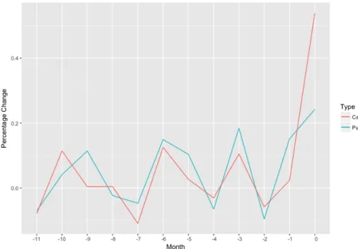
Figure 1.1: Percentage Changes of Option Volume for 12 Months (Upward-Jump)

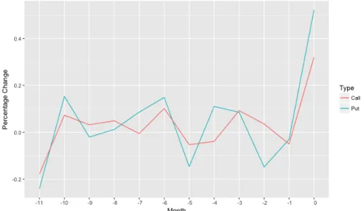
My main hypothesis is that an informed trader who has pessimistic expectations about the future buys put options to secure her positions. Intuition for this statement comes from the definition of put option. Usage of call options would follow the same logic. Figure 1.1 and Figure 1.2 displays the intuition. Month-zero represents the month in which returns make a larger move (i.e. downward-jump or upward-downward-jump). It is clear that there is a significant peak in put and call option trading prior to month-zero. Especially, call options increase is more pronounced prior to upward-jump movement and put options volume increase is more pronounced before crash months. Hence when I forecast the likelihood of a crash (jump), I would expect call(put) options to have negative(positive) impact on it. Thus, my hypotheses are:

H1: Volume of call option is negatively related to a crash. H2: Volume of put option is positively related to a crash. H3: Volume of call options is positively related to a jump.

H4: Volume of put option is positively related to a jump.

Options literature suggests implied volatility also contain significant information relevant for stock market. Implied volatility is a forward looking measurement of stock risk which is calculated from option prices; hence they are referred to as price-based measures. Bali & Hovakimian (2009), Cremers & Weinbaum (2010), Xing et al. (2010), and Doran & Krieger (2010) investigate the link between di↵erent implied volatility measures and expected stock returns. They find a significant relation between call and put options implied volatility and future stock returns. Volume part of the literature (Roll et al. (2010), Johnson & So (2012)) shows that ratio of options volume to stock volume predict negative future stock returns. Economics rationale of this is that the prediction power of options market comes from its leverage advantage (Ge et al. (2016)). Moreover, this ratio is also used as a proxy for informed traders in options market. I use these measures as control variables in my model.

To investigate the hypotheses stated above, I use a comprehensive monthly op-tions market dataset which spans the period between 1996 to 2015. Final version of the data has 219, 312 firm-month observations and 2778 individual firms. To my knowledge, this is the most extensive dataset in terms of number of observa-tions and individual firms. It also enables me to validate previous results provided by much narrower datasets in previous literature. Moreover, I follow Marin & Olivier (2008)’s definitions of crash and jump: A firm’s stock return crash vari-able (jump) in a given month is equal to one if the di↵erence between the return, in that month, and average return of previous 60-months is less (more) than 2 standard deviations of prior returns and zero otherwise. I use above price-based measures as control variables. I analyze crash and jump variables in di↵erent models. Finally, using a logit model, I predict the likelihood of crash and jump with call and put options volume, price-based measures, and volume ratio.

Figure 1.2: Percentage Changes of Option Volume for 12 Months (Downward-Jump)

Findings are summarized as follows: (1) Implied volatility determines large neg-ative movements of stock prices. Before a crash, investors prefer to buy out-of-money put options which boost its implied volatility. Variables which capture this feature have significant positive relation with the likelihood of a crash. (2)

Volume of put and call options, also, determines large negative movement in con-trast to previous literature. While the relation between put options volume and crash is positive, it is negative for call options volume. Moreover, put volume has a higher predictive power than call volume on crash variable. (3) Before a jump, investors become reluctant to trade in options market. Earlier forecasting capability of price-based variables became insignificant. However; volumes of put and call options stay relatively significant. Again, put volume has a positive sign while call volume has negative for jump variable. The second result is consistent with H1 and H2; however, because of signs, the third result refutes H3 and H4. I can attribute results for jump model to Marin & Olivier (2008) and Veronesi (1999). Marin & Olivier (2008) show that insider do stay in the market before a significant upward movement of stock prices. For my case, this may mean that informed traders switch to stock market as well. Other investors who have am-biguities about the direction of price movements stay in options market and this leads to similarly signed significance in put and call volume variables. Further, Veronesi (1999) documents that investors have asymmetric attention to news. Market overreacts to bad news, but it underreacts to good news. My finding is consistent with the Veronesi (1999) model in that informed traders underreact to jumps, i.e. good news.

The rest of the thesis is organized as follows: Chapter 2 examines relevant and recent part of the literature on given topic in details, Chapter 3 introduces data, variables and their measurements. Chapter 4 gives the results. Finally, Chapter 5 concludes the thesis.

CHAPTER 2

LITERATURE REVIEW

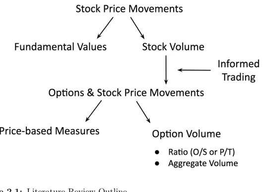
Figure 2.1 shows the outline of this literature review. Prediction of stock price movement has been widely studied from various perspective. One side of the literature studies use fundamental values, such as accounting variables, of a firm to forecast large movements in its stock prices. Other side use stock trading volume as an explanatory variable to explain stock returns. Another strand of the literature explores the information content of options market for stock prices. The intuition here is that there are informed traders in options market, hence they should have information about the direction of stock prices. To document this claim, researchers use price-based measures and/or options volume measures. My research lies on this part. I use both of the measurements to explain large stock price movements at firm level.

The research on stock price movements and stock volume dates back to 60s. Ying (1966) finds that an increase (decrease) in daily trading volume is followed by an increase (decrease) in the price of stocks. Many years later, Gallant et al. (1992) extend Ying (1966) paper by studying a larger dataset which extends from 1928 to 1987. They reach the same conclusion that high stock trading volume causes large stock price movements. Moreover, they demonstrate a positive risk-return relationship with lagged stock volume variable. Campbell et al. (1993) only look at correlations between stock return and trading volume without any prediction

Figure 2.1: Literature Review Outline

and conclude high-volume is more correlated with negative returns than low-volume. Gervais et al. (2001) follow this idea and show that unusual high(low) stock volume is followed by a positive(negative) excess return. Chen et al. (2001) apply cross-sectional regressions with trading volume and past returns to predict negative skewness with respect to Hong & Stein (2003) theoretical model on heterogeneous beliefs.

Following this literature, Marin & Olivier (2008) employ a di↵erent approach on the issue. They use a special dataset which contains insider purchase and sell volume of individual stocks. They hypothesize that volume of insider trading has a relationship with stock price movements. They introduce two variables (crash and jump) to represent direction of the movements in order to examine the behavior of insiders before each direction. They find that insiders purchase volume decreases many months before a significant downward movement whereas this is not the case before an upward spike in stock prices. In my analysis, I try to forecast the crash and jump variables that Marin & Olivier (2008) use; but from options market perspective. My study di↵ers from Marin & Olivier (2008)

in terms of explanatory variables. I use options volume along with price-based measures and option-stock volume ratio as control.

Before this thesis, there is a well established literature which explores the link between stock returns and options market variables. Black & Scholes (1973) and Easley et al. (1998) assert that option traders take advantage of liquidity and leverage of the market. They claim that these investors are more sophisticated than an average trader and refer to them as informed traders. After this def-inition, researchers claim a link between behavior of these particular investors and stock price movements. Intuition is that, because they have information ad-vantage, they should act on it. One segment of these researchers study implied volatility of options market to predict future stock returns. Others, on the other hand, look at the options volume for information.

First subdivision concentrates on options prices as a predictive tool for large movements in stock prices. Doran et al. (2007) introduce moneyness-based1 mea-sures to study implied volatility. Their intuition comes from the fact that since investors are likely to hedge before a downward crash, they are willing to pay extra premium for OTM-put options in order to protect their positions. And the idea applies for upward spike with OTM-call options. They examine the informa-tion content in S&P100 opinforma-tions index by creating separate models for downward and upward jumps as in the case of Marin & Olivier (2008). They demonstrate that implied volatility spread between OTM-put and ITM-put (or ATM-put) has a positively significant link to likelihood of a downward crash. Moreover, implied volatility spread between OTM-call and ITM-call (or ATM-call) predicts a crash with a significant negative coefficient. However, neither call options spread nor put options spread can predict an upward spike of stock prices. They do not have an explicit explanation for this perplexing result. Although, they pointed

1_{Moneyness category defines how much the option is in or out of the money. When a call} option is 1) at-the-money (ATM) its underlying stock price is equal to, 2) in-the-money (ITM) stock price is greater than, 3) out-of-money (OTM) stock price is less than strike price, i.e., agreed upon price. And these are reverse for put options, except ITM.

out that investors may be more concerned about negative movements than posi-tive movements.

Bali & Hovakimian (2009) use implied volatility spread between ATM-call and ATM-put as a proxy for jump risk and show that the spread has a significant positive relation with expected stock returns. In addition, they show an infor-mational spillover e↵ect and interpret it as the existence of informed traders in options market. Later, Cremers & Weinbaum (2010) use the same volatility spread and verify Bali & Hovakimian (2009) findings by using weekly stock re-turns. Furthermore, they also assert that the deviation of option prices from put-call parity constitutes a proxy for informed traders. This implied volatility measure is one of explanatory variables in my model.

Xing et al. (2010) define another implied volatility spread and call it skew or smirk.2 _{Skew is the implied volatility spread between put-OTM and call-ATM}

options. The idea here is that investors buy more put-OTM options when they are in fear for future, thus put-OTM become more expensive compared to call-ATM. They hypothesize that the spread should predict downside jump of stock prices. Results support the hypothesis with a significant negative link between the spread and stock returns. Volatility smirk is another price-based variable in my model.

Later, Doran & Krieger (2010) separate volatility skew into two parts which capture distinct information about stock returns. One part is proxied by implied volatility spread between OTM-call and ATM-call. The intuition here is that when investors have optimistic expectation about market’s future, they trade with OTM-call options; hence it becomes more expensive compare to ATM-call. The second part is implied volatility spread between OTM-put and ATM-put. The idea here is similar to previous spread with one di↵erence, that is, investors

2_{Bates (1991) introduced the volatility skew measure and tested it on the year prior to 1987} market crash. He found that skew is unrelated to crash. Gemmill (1996) used skewness on London’s FTSE 100 index and found no relation between skewness and crash neither.

trade with OTM-put options when they have pessimistic expectations. They find a positive(negative) significant link between stock returns and call-spread (put-spread). Besides, they come up with another spread measure between OTM and ITM options. The spread captures the tails of volatility skew by representing whether the smile is forward or reverse skewed. When they run it to forecast stock return, they find a significant positive relationship.

Fu et al. (2016) provide extensive review about price-based measures. They claim that existing studies have conflicting results about the significance of each mea-sure. Therefore they test the measure in a multivariate model and find that volatility skew has the highest significance among other measures while forecast-ing stock returns. In my research settforecast-ing, all the measures in Fu et al. (2016) are used except realized volatility. My research di↵ers in two ways from theirs: (1) I forecast the likelihood of a large movement of stock prices with two di↵erent models; herein (2) main variables are call and put option volumes. I do not try to document the significance of price-based measure but to use them as control variables.

Other part of options literature explores the link between stock and options mar-ket by focusing on the direction of traders. To proxy for the direction, Roll et al. (2010) introduce a ratio of aggregate options trading volume and stock trading volume. Johnson & So (2012), Ge et al. (2016) show the predictive power of this ratio on individual stock returns. A recent paper by Han et al. (2017) in-troduces two new option volume ratios. One of them is the ratio of OTM-put volume to total OTM options. The other one is the ratio of OTM-call volume to total OTM options volume. They test these ratios along with Xing et al. (2010)’s volatility skew to predict stock returns. They point out the importance of investors’ motivations while trading in options market. Their claim is that investors have two methods of trading available to them; Directional trading (i.e. volume-based) and Volatility trading (i.e. volatility-based). The method used

depends on investors’ future expectations on upward and downward movements of the stock prices. When main motivation is volatility, volume ratio loses its significance; when directional information is the motivation, high volume ratio is the predictor of negative future prices. At the end, their results support the idea OTM-put volume predicts negative stock returns whereas OTM-call volume fails to do so.

Some studies examine whether above links are more pronounced during an an-nouncement or not. Cao et al. (2005) look at the information in call volume imbalance before takeover announcements and find that call (buyer and seller initiated) volume has information prior to the event; Spyrou et al. (2011) do the same analysis on UK options market and reach similar results. Gharghori et al. (2017) look at implied volatility prior to stock-split announcements. Atilgan (2014) and Truong et al. (2012) examines implied volatility around earnings an-nouncements. This literature assumes there is large information asymmetry prior to events, news, or announcements. Therefore, I check my hypotheses against this view with a robustness analysis. I conduct a sub-sample analysis, in which obser-vations with earnings announcement are excluded, to check whether the results from full sample analysis hold or not.

To conclude, I have established my research on various literature. Hence, my research forms a nexus of relationship between di↵erent perspectives. This mul-tifaceted approach to explain the link between volume of options in conjunction with price-based measures make this thesis unique.

CHAPTER 3

DATA AND METHODOLOGY

3.1 Data

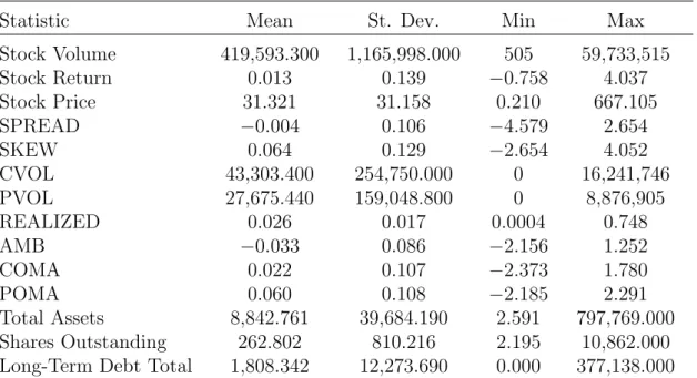
I obtain options data from Option Metrics database which gives volume, open interest, end-of-day bidask quotes for U.S. stocks. The sample period is from January 1996 to December 2015. Return data is provided by the Center for Re-search in Security Prices (CRSP). Securities are common stock which is collected by CRSP share code 10 and/or 11. For firm-level accounting variables, I use COMPUSTAT data. After merging two sets, I omit observations (firm-month) with: (1) number of months for a firm is less than 60 months, (2) stock price is less than $2. Table 3.1 gives a thorough descriptive statistics of the dataset.

3.1.1 Dependent Variables

Dependent variables are from Marin & Olivier (2008). It captures an unusual move (up or down) of a firm’s stock return in a month by comparing the return with its previous 60 months returns rolling average standard deviation.

CRASH : It takes value of 1 when return of the given month is 2 standard devia-tion away to negative side, otherwise its value is equal to 0:

Table 3.1: Summary Statistics

Statistic Mean St. Dev. Min Max

Stock Volume 419,593.300 1,165,998.000 505 59,733,515 Stock Return 0.013 0.139 0.758 4.037 Stock Price 31.321 31.158 0.210 667.105 SPREAD 0.004 0.106 4.579 2.654 SKEW 0.064 0.129 2.654 4.052 CVOL 43,303.400 254,750.000 0 16,241,746 PVOL 27,675.440 159,048.800 0 8,876,905 REALIZED 0.026 0.017 0.0004 0.748 AMB 0.033 0.086 2.156 1.252 COMA 0.022 0.107 2.373 1.780 POMA 0.060 0.108 2.185 2.291 Total Assets 8,842.761 39,684.190 2.591 797,769.000 Shares Outstanding 262.802 810.216 2.195 10,862.000 Long-Term Debt Total 1,808.342 12,273.690 0.000 377,138.000

CRASHi,t =

⇢ 1, if ERi,t ERi,t  2 i,t

0, otherwise

(3.1)

JUMP : It takes value of 1 when return of the given month is 2 standard deviation away to positive side otherwise its value assigned as 0:

JU M Pi,t =

⇢ 1, if ERi,t ERi,t 2 i,t

0, otherwise

(3.2)

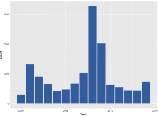
Figure 3.1 and Figure 3.2 show cumulative number of crashes and jumps, respec-tively, for each year by calculating dependent variables. There are 3 years, during which frequency of crash and jumps is significantly higher than others. Numbers peak in 2001, 2008, and 2009 related to dotcom bubble and US subprime mort-gage crisis.

Figure 3.1: Number of Crashes per Year 3.1.2 Independent Variables

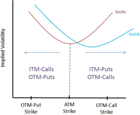
Before dwelling into variable definitions let me explain what is volatility smile and smirk and why it is related. Volatility smile is discovered after stock market crash in 1987. Before that, Black-Scholes model assumes a constant implied volatility with respect to strike price. However, due to the changes in investors behaviors with a fear of crash, out-of-money and in-the-money put&call options become important. Fear of crash causes an increase in option prices, hence an increase in their implied volatility. Figure 3.3 depicts the smile. As strike price of OTM-puts and ITM-calls decreases their prices increase. For ITM-OTM-puts and OTM-calls, this e↵ect is the opposite. Smile is called smirk (or skew) when weight of one side is more than the others. Figure 3.3 shows only reverse skew which refers to higher implied volatility for left hand side. The opposite, forward skew, is also possible. Then, right hand side has the higher volatility. When investors have bad expectation about the future, forward skew exists. Positive expectations, on the other hand, generate reverse skew. The reason why this is important is that

Figure 3.2: Number of Jumps per Year

most of the independent variables exhibit a particular part of volatility smile. I follow Doran & Krieger (2010) explanations on these parts.

Using an algorithm based on Cox et al. (1979), OptionMetrics constructs the standardized implied volatility surface data with a kernel smoothing technique described in the manual. I focus on end-of-month options with one month to expiration and categorize options as in-the-money, at-the-money and out-of-the-money based on their deltas. Most of the papers that I have mentioned use strike-price to stock-price ratio to determine moneyness level; however as Bollen & Whaley (2004) point out the ratio also depends on volatility of the underlying asset and time to expiration of its option. Therefore, I follow Bollen & Whaley (2004) and use option’s delta (Black & Scholes (1973)) to set the categories:

c = N



ln((S D)erT_{/K) + 0.5} 2_T

p

T (3.3)

level. K is exercise and T is time to expiration of the option. r is risk-free rate. is the standard deviation. Finally, N is normal density function. At-the-money options have delta as 0.5 and 0.5 for call and put, respectively. In-the-money options have delta as 0.2 and 0.2 for call and put, respectively. For out-of-the-money options, we choose delta as 0.7 and 0.7 for call and put, respectively. I use these levels to calculate implied volatility related independent variables: SPREAD: This measure is taken form Bali & Hovakimian (2009). The idea there is to show a demand increase in options will result an increase in their implied volatility. Furthermore, if there is a jump(crash) in future for a stock, then demand for its call(put) should increase; hence spread variable defined below represents a one-sided expected increase in stock prices. This is the middle of volatility smile (Doran & Krieger (2010)). CV olAT M is the average of implied volatility of ATM call options at the end of previous months. P V olAT M _{is the}

put version of former calculation:

SP READ = CV olAT M P V olAT M (3.4)

Cremers & Weinbaum (2010) have the same measure; but they use weekly average returns.

SKEW : Volatility is, again, the average of implied volatility of OTM-put and ATM-call at the end of previous months (it is weekly average in Xing et al. (2010)). The reason for choosing ATM call options is that ATM calls are the most liquid ones compare to its OTM counterpart and also it captures the expectations commonly held by investors; thus it is good way to measure informed traders activity. Doran & Krieger (2010) refers to this measure as the left (put side) and middle (call side) of volatility smile:

Figure 3.3: Volatility Smile and Smirk

SKEW = P V olOT M _{CV ol}AT M _(3.5)

AMB, COMA, POMA: Doran & Krieger (2010) have three measures: (1) above-minus-below shows the di↵erence between implied volatility of options which min-uend is K > S1_{and subtrahend is K < S. COMA and POMA are complementary}

to each other and called out-of-minus for call and put options respectively. They present AMB as tails of the smile; COMA as right and middle side of the smile for calls; POMA as left and middle for puts. All implied volatility are the monthly average of previous month.

AM B = (P V ol

IT M_{+ CV ol}OT M_{) (CV ol}IT M _{+ P V ol}OT M₎

2 (3.6)

COM A = CV olOT M CV olAT M (3.7)

P OM A = P V olOT M P V olAT M (3.8)

REALIZED: It is the volatility of past monthly returns. Implied volatility shows market’s expectation about future whereas realized volatility shows what hap-pened in the past. I use this variable in robustness check.

CVOL: This is the monthly cumulative (buy and sell) volume of call options. I take the natural logarithm of the dollar trading volume to prevent positive skewness e↵ect.

PVOL: This is the monthly cumulative (buy and sell) volume of put options. Same as CVOL variable, I take the natural logarithm here as well.

3.1.3 Control Variables

I use control variables to remove possible e↵ects on the significance of results. There are already well-defined firm-level variables in the literature:

O/S : This is the ratio of aggregate options volume to stock volume. It represents the direction of investors between two markets. If it is higher than 1, it means investors are in options market. If it is less than 1, then most of the traders are in stock market. This variable also used as informed trader indicator. (Roll et al. (2010)).

SIZE : Market value of stock at the end of the year. I take natural logarithm before using it (Chen et al. (2001)).

RETURN : Lagged returns of the equity. I use 1 month (RET U RNi,t 1), 2

months (RET U RNi,t 2), and 3 months (RET U RNi,t 3) lagged returns (Chen

et al. (2001)).

LEVERAGE : It is the ratio of total long-term debt to total assets (Chen et al. (2001)).

3.2 Methodology

I run the followings regressions:

CRASHi,t = 0+ 1CV OLi,t 1+ 1P V OLi,t 1+ 2SP READi,t 1+

3SKEWi,t 1+ 4AM Bi,t 1+ 5COM Ai,t 1+ 6P OM Ai,t 1+

CON T V ARIABLES + ✏i,t

(3.9)

JU M Pi,t = 0+ 1CV OLi,t 1+ 1P V OLi,t 1+ 2SP READi,t 1+

3SKEWi,t 1+ 4AM Bi,t 1+ 5COM Ai,t 1+ 6P OM Ai,t 1+

CON T V ARIABLES + ✏i,t

(3.10)

where i denotes an individual firm, t denotes month and ✏ is the error term. Following Marin & Olivier (2008), I perform conditional logit with fixed e↵ects regression for the estimation. Choice of logit, instead of probit, relies on the fact that probit gives biased results with fixed e↵ects specification for panel data (Greene (2002)).

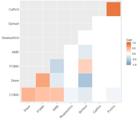
As it is pointed out in Bollen & Whaley (2004) and Han et al. (2017), trades that are based on volatility and volume information are not necessarily correlated. Hence, they must have di↵erent level of predictive powers. Figure 3.4 shows the correlation matrix between volatility and volume variables. White regions refer to correlation coefficients that are very close to zero. Therefore, it is safe to place volume and volatility based variables on the right hand side of the regression.

CHAPTER 4

EMPIRICAL RESULTS

Table 4.1 and Table 4.2 provide main results for CRASH and JUMP respectively. I run multivariate as well as univariate regressions with the whole sample. The reason for univariate regressions is to provide another evidence for previous lit-erature on implied volatility and to see whether the dependent variables that I use are consistent with the literature or not. After that, I run the multivariate regressions to test my hypotheses about options volumes with the existence of price-based variables and O/S ratio. In total, I have eight main independent variables and four control variables. I should note that because of how they are calculated1_{, SPREAD, POM, and SKEW are linearly dependent. Therefore,}

there are three multivariate regressions with di↵erent combinations. Regression (6) shows results with SKEW and SPREAD while (7) uses POMA and SPREAD. Finally, regression (8) depicts overall e↵ects with SKEW and POMA.

Main purpose of this thesis is to test whether volume of options can predict the likelihood of a large movement or not. However, design of my models allows us to comment on the literature of investor behavior. I have two independent variables, CRASH and JUMP, to explore the symmetrical behavior of investors in options market. CRASH indicates that a firm experiences a large negative movement with respect to its past sixty month returns. JUMP, on the other hand, represents the large positive movement. With this in mind, my expectations on explanatory

variables should reflect assumed symmetrical relationship across models. In other words, the signs should be opposite for two cases.

SPREAD is the di↵erence between implied volatility of ATM-call and ATM-put options. What I expect is that before a jump the demand for ATM-calls should increase; hence its volatility should increase. This leads to a positive significance for SPREAD before a jump. For the crash case, demand for ATM-put increases, then its sign should be positive and significant before a crash. Nevertheless, these are at-the-money options. They should not have very significant results in multivariate regressions because of variables which represent the OTM options. In addition to that, ATM options reflect the view of common investors. SKEW is the spread between implied volatility of OTM-put and ATM-call options. I expect that OTM-put options should attract most of informed traders’ attentions compared to other options types in an expectation of a crash. The sign for the should be opposite for the jump. I anticipate SKEW variable to be positive and significant in the CRASH regressions and negative and significant in JUMP regressions.

Moreover, I use AMB, COMA and POMA to represent the di↵erent e↵ect of volatility smile on stock prices. COMA and POMA are complementary to each other. COMA indicates the informed traders in call options, while POMA does it for put options. As I mentioned before ATM options represent average in-vestors’ views. Hence, Doran & Krieger (2010) say that we should expect that the ones who trade with OTM options should be the investors with information. Thus, COMA and POMA should have positive significant coefficients in JUMP and CRASH regressions respectively. Besides in order to reflect the symmetric behavior of investors, COMA and POMA should have opposite signs for the op-posite models. Doran & Krieger (2010) state that AMB represents the tails of volatility skew. We can interpret it as the di↵erence between right and left hand side in Figure 3.3. When investors are expecting negative news, they will go to

the right side of the figure and increase its volatility; hence the negative of the di↵erence will be augmented. Therefore, before a crash a negative coefficient is expected. As mentioned earlier, I base these expectations on the assumption of symmetric behavior of traders before good and bad news.

Regression (1) in Table 4.1 shows slope coefficient on SPREAD as negatively sig-nificant at 1% level. SPREAD represents excess demand for ATM-call options. Negativity comes from the fact that investors desire for ATM-calls falls in crisis time. SKEW in regression (2), on the other hand, emphasizes on OTM-put op-tions relative to ATM-calls. With the same logic, investors secure their trades with OTM-puts before a crash. And it is positively significant at 1%. In regres-sion (3), AMB ’s significance level is 1% and its coefficient is positive. In regresregres-sion (4), COMA has negative coefficient with 1% significance level. In contrast with Doran & Krieger (2010) I find a significant COMA for both dependent variables. Furthermore, COMA is significant in three multivariate regressions as well. In-vestors’ demands for OTM-calls decrease in crash times; hence the coefficient is negative. Finally, in regression (5) POMA’s coefficient is 7.511e 01 and its t-value is 2.996. As I have explained in Chapter 3, POMA is opposite of COMA, that is, it shows excess demands for OTM-put options. It is less significant, at 5%, than the rest.

In multivariate regressions, I add CVOL and PVOL to test the hypotheses. I use aggregate volume of call and put options separately. In contrast to Fu et al. (2016), I find significant results with both volumes. Call options volume is nega-tive and significant at 10% level in all multivariate regressions while put options volume has positive slopes throughout the regressions and significance level at 5%. This suggests that before a crash investors trade with put options and in-crease its volume. Negative coefficient on call options volume implies that when there is a decrease in demand of call options, the likelihood of a crash increases. Investors use put options for security purposes in crisis times.

I expect O/S ratio to be positively significant since I assume that informed in-vestors trade in options market before a large movement in stock prices. Re-gressions for CRASH variable -reRe-gressions (6), (7), and (8)- the ratio is positive and significant at 1% level. It suggests that investors go into options market before a downward movement in prices. What they do in the market is revealed in other explanatory variables. PVOL and CVOL have significant levels at 10% and 5% respectively. Furthermore, their signs support hypotheses H1 and H2, which are call volume decreases and put volume increases before a crash. The result is also intuitive since investors use put volume to protect their positions. In addition, AMB, POMA, SKEW show that investors trade with OTM-put options. However; information of whether they are selling or buying cannot be determined from this dataset. In regression (6), SPREAD loses its significance due to SKEW. SKEW has positive slopes and significance levels at 1%. The re-sults are consistent with the literature. SKEW exploits POMA’s significance as well in regression (8). Fu et al. (2016) also find that SKEW has larger predictive power than other variables. My findings support this view. In regression (7), absence of SKEW gives power both to SPREAD and POMA. Their coefficients’ signs stay same and significance levels are at 1%. AMB, on the other hand, loses its significance entirely. It is understandable since both SPREAD and SKEW have similar information with AMB.

Table 4.2 demonstrates the relationship between JUMP variable with given ex-planatory variables. SPREAD in regression (1) is positively significant at 5% level. The result is consistent with the literature. Some papers (e.g. Fu et al. (2016) ) show that implied volatility spread has a positive relation with stock returns; hence spread should, and it does, increase before a large jump in stock prices. Even though SKEW is no longer significant, it keeps the logic by its negative coefficient. Negative sign points out that investors do not pay excess premium for OTM-put and ATM-call when they are in optimistic expectations. This interpretation can also be supported by the insignificance of COMA variable.

T a bl e 4 .1 : R eg re ss io n An al y si s of C R AS H V ar ia b le D ep endent var iable: C R AS H (1) (2) (3) (4) (5) (6) (7) (8) P R E AD 8. 530 e 01 ⇤⇤⇤ -1. 332e-01 1. 442 e +0 0 ⇤⇤⇤ (-3.902) (-0.363) (-6.212) KEW 1. 30 4e+ 00 ⇤⇤⇤ 1. 309 e +0 0 ⇤⇤⇤ 1. 445 e +0 0 ⇤⇤⇤ (5.628) (3.541) (6.245) OL 9. 093 e 07 ⇤ 9. 456 e 07 ⇤ 9. 965 e 07 ⇤ (-2.345) (-2.596) (-3.145) OL 1. 578 e 06 ⇤⇤ 2. 934 e 06 ⇤⇤ 1. 194 e 06 ⇤⇤ (3.258) (4.037) (2.966) B 1. 908 e +0 0 ⇤⇤⇤ -4 .2 68 e-01 -6 .9 30 e-01 -3 .9 03 e-01 (-7.026) (-0.874) (-1.937) (-1.036) 1. 314 e +0 0 ⇤⇤⇤ 1. 951 e +0 0 ⇤⇤⇤ 2. 458 e +0 0 ⇤⇤⇤ 1. 156 e +0 0 ⇤⇤⇤ (-5.473) (-4.665) (-6.034) (-4.194) 7. 511 e 01 ⇤⇤ 1. 309 e +0 0 ⇤⇤⇤ -1. 332e-01 (2.996) (3.541) (-0.363) 4. 238 e 02 ⇤⇤⇤ 4. 019 e 02 ⇤⇤⇤ 5. 109 e 02 ⇤⇤⇤ 5. 091 e 02 ⇤⇤⇤ 6. 429 e 02 ⇤⇤⇤ 5. 439 e 02 ⇤⇤⇤ 3. 309 e 02 ⇤⇤⇤ 3. 934 e 02 ⇤⇤⇤ (5.116) (5.087) (6.168) (6.189) (5.466) (6.384) (5.293) (5.239) E T UR N -2 .2 56 e-01 -2 .3 32 e-01 -2 .1 70 e-01 -2 .2 56 e-01 -2 .0 45 e-01 -2 .5 20 e-01 -2 .5 20 e-01 -2 .5 20 e-01 (-1.109) (-1.146) (0.202 ) (-1.067) (-1.107) (-1.234) (-1.234) (-1.234) IZE 1. 22 8e-0 1 1. 14 5e-0 1 1. 195 e-0 1 1. 38 6e-0 1 1. 17 3e-0 1 1. 19 3e-0 1 1. 18 8e-0 1 1. 08 6e-0 1 (0.233) (0.015) (0.127) (0.372) (0.091) (0.119) (0.112) (0.098) E VE R A G E 1. 07 8e -0 1 9. 58 1e -0 2 8. 37 8e -0 2 1. 00 9e -0 1 1. 04 7e -0 1 1. 12 4e -0 1 1. 12 4e -0 1 1. 12 4e -0 1 (0.354) (0.315) (0.275) (0.331) (0.344) (0.369) (0.369) (0.369) ations 84,018 84,018 84,018 84,018 84,018 84,018 84,018 . P ossi b le R 2 0.118 0.118 0.118 0.118 0.118 0.118 0.118 Lik eliho o d -5,268.687 -5,261.791 -5,254.893 -5,262.630 -5,270.988 -5,176.541 -5,144.329 ote: ⇤ p < 0.1; ⇤⇤ p < 0.05; ⇤⇤⇤ p < 0.01

COMA describes excess demand for OTM-call options compare to ATM-call op-tions. In regression (3), 1% significant and positive AMB implies a forward skew which means volatility for higher strike price is greater than lower strike price op-tions’ implied volatility. Image of forward is exactly opposite of volatility skew. This suggests that OTM-call and ITM-put options have higher demand in the market before a jump in stock prices. Result of POMA in regression (5) endorses this demand approach; since it documents the insignificance of other put options types.

Generally, traders who use OTM-option tend have higher expectations than ITM-option traders about a large movement in the future. Because using ITM ITM-options does not mean a definite profit if you are in a positive expectations about the underlying price. ITM-put give profit only when underlying price is less than its option’s strike price. Hence in order an investor to trade with ITM-put, she should not expect an increase in stock prices. But since this is the jump model, this conclusion implies that the majority of investors in the options market are not informed. The explanation for this conflict lies in O/S variable which represents the direction of investors between stock and options market. While the ratio is positively significant in CRASH regressions, in Table 4.2 it is negatively significant at 1% level. It suggests that informed traders go back to stock market before a large upward movement in stock prices. The idea may be attributed to Marin & Olivier (2008) jump result. They show that insiders do not leave stock market before a large positive movement in stock prices, they trade in stock market. Therefore, the same story can be valid here. It maybe the case that some of the informed traders go back to stock market before an positive event. Another explanation can be related to the investor attention literature. It explores the e↵ect of attention on firms and their stock prices in general. If a firm is popular, in other words, get lots of attention from traders its valuation become easy. In contrast, if investors give less attention to a particular firm, news about

that firm underrated by the investors. Veronesi (1999) contributes this literature by giving a theoretical model to show that investors has asymmetric attention to bad and goods news regardless of the popularity of a firm. They claim that investors stay neural prior to a positive event. Andersen et al. (2003) and Mondria et al. (2012) support Veronesi (1999) model by using dataset of exchange rate and equity market respectively. Hence, this implies that traders in options market may also act in this way. Instead of changing their position to adjust a positive event, that is, large upward movement in stock prices, they do not. Thereby, we would reach a result like in my jump model.

Due to lack of signed volume data, I cannot test symmetry related predictions of the models cited above. But my results support H1, H2 and rejects H3 and H4 and suggest that investors do not behave alike before an upward and downward stock price movement.

4.1 Robustness Check: Earnings Announcements

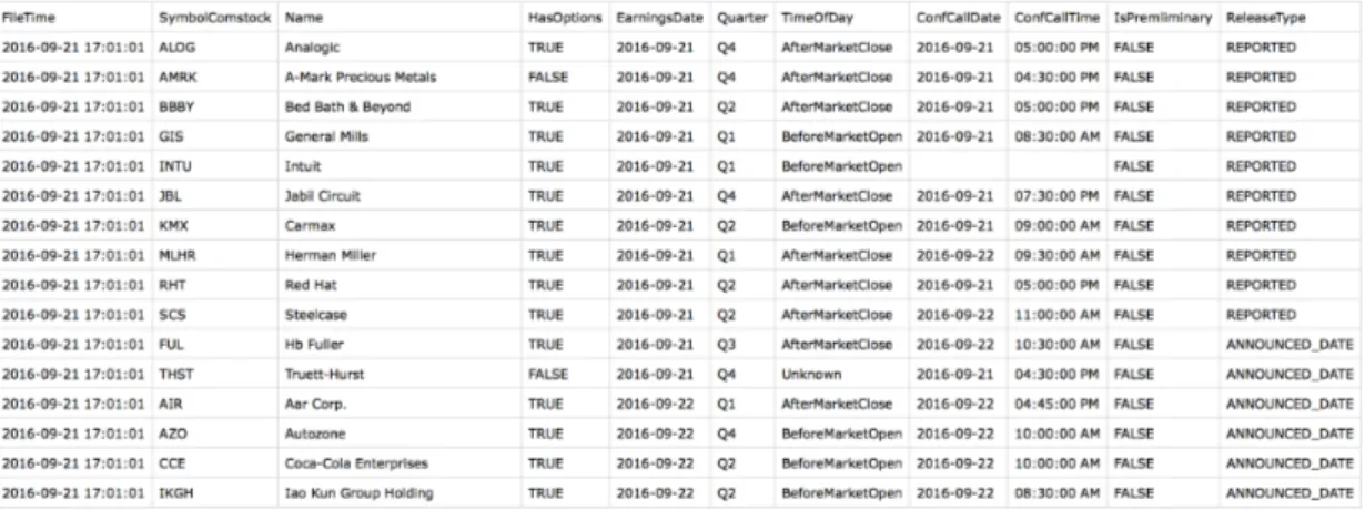
Calendar e↵ect is a hypothesis which claims that particular months, days may cause above or below average price change in stocks. Hence, these particular times may provide useful information about a firm’s well-being and may repre-sent bad or good news about a firm. One of the most studied calender e↵ect is earnings announcement and I test my hypothesis against this alternative expla-nation. Earnings announcement hypothesis claims that large price movements in a given month can be the reason of released earnings numbers. If it is the case, when I take out announcement dates from my sample the significance of explana-tory variables should vanish. On the other hand, if the hypotheses are valid, then the predictive power of explanatory variables should hold for the subsample too. Earnings announcement data are gathered from COMPUSTAT and Market Chameleon data. Figure 4.1 shows a snapshot from this dataset. There

T a bl e 4 .2 : R eg re ss io n An al y si s of JUM P V ar ia b le D ep endent var iable: JUM P (1) (2) (3) (4) (5) (6) (7) (8) S P R E AD 4. 912 e 01 ⇤⇤ 7. 229 e 02 ⇤ 4. 854 e 01 ⇤ (2.760) (2.212) (2.073) S KEW 4. 865 e 01 -2.383e-01 -3.1 06e-01 (-0.624) (-0.662) (-1.320 ) CV OL -4. 406e-08 1. 076 e 06 ⇤ -6. 604e-07 (-5.546) (-2.426) (-1.620) PV OL 1. 524 e 06 ⇤⇤ 1. 945 e 06 ⇤⇤ 1. 115 e 06 ⇤ (3.079) (3.403) (2.346) AM B 1. 005 e 02 ⇤⇤⇤ 6. 935 e 01 . 7. 699 e 01 . 4. 543 e 01 . (3.967) (1.653) (1.844) (1.293) COMA 1. 062 e 02 6. 093 e 01 . 4.485e-01 6. 324 e 01 . (0.155) (1.753) (1.287) (1.789) POMA -8. 794e-02 -5. 49 0e-01 7. 229e-02 (-0.383) (-1.508) 0.212 O/S 4. 239 e 02 ⇤⇤⇤ 4. 018 e 02 ⇤⇤⇤ 3. 192 e 02 ⇤⇤⇤ 3. 029 e 02 ⇤⇤⇤ 4. 025 e 02 ⇤⇤⇤ 3. 402 e 02 ⇤⇤⇤ 2. 023 e 02 ⇤⇤ 3. 902 e 02 ⇤⇤ (-5.353) (-4.302) (-5.782) (-5.532) (-5.202) (-5.102) (-3.340) (-3.993) R E T UR N -2 .3 55 e+ 00 -2 .3 52 e+ 00 -2 .3 64 e+ 00 -2 .3 72 e+ 00 -2 .3 60 e+ 00 -2 .5 47 e-01 -2 .8 99 e+ 00 -2 .6 75 e+ 00 (-1.905) (-1.893) (-1.008) (-1.047) (-1.964) (-2.945) (-1.919) (-1.619) S IZ E -1 .8 50 e-01 -1 .8 13 e-01 -1 .8 92 e-01 -1 .8 20 e-01 -1 .8 47 e-01 -1 .7 89 e-01 -1 .4 56 e-01 -1 .2 56 e-02 (-0.666) (-0.405) (-0.896) (-0.474) (-0.605) (-0.291) (-0.267) (-0.145) L E VE R A G E 7. 924 e 01 7. 984 e 01 7. 705 e 01 7. 813 e 01 7. 876 e 01 6. 283 e 02 8. 255 e 01 7. 245 e 01 (0.366) (0.390) (0.274) (0.319) (0.347) (0.504) (1.12 9) (0.511) Observ ations 84,018 84,018 84,018 84,018 84,018 84,018 84,018 Max . P ossi b le R 2 0.154 0.154 0.154 0.154 0.154 0.154 0.154 Log Lik eliho o d -6,864.180 -6,864.464 -6,860.495 -6,856.057 -6,867.729 -6,698.816 -6,685.073 N ote: ⇤p < 0.1; ⇤⇤p < 0.05; ⇤⇤⇤ p < 0.01

Figure 4.1: Snapshot from Earnings Announcement Dataset

are several caveats associated with this dataset. Earnings announcement days(EarningsDate) and conference call days(ConfCallDate) are not always the same even though the snapshot makes it seem so. The reason is that some com-panies do not hold conferences. Instead, they issue earnings through 10-K and/or 10-Q reports via SEC. Furthermore, it is important to mention that dataset con-tains information on whether the announcement is preliminary or not. In other words, some firms issue earnings information before the scheduled date. To take that into consideration, I assign preliminary date as the announcement date if preliminary date is in the same month with official announcement date. Fi-nally, to test the hypothesis, I merge earnings announcement information with my dataset and then delete the observations(i.e., firm/month) if the given row has announcement date in given month.

The result is as expected. Significance of explanatory variables stays at similar level as main regressions results. Table 4.3 shows the result of regressions when JUMP is the dependent variables. Even though, most of the variables keep their significance level t-values of AMB and PVOL decrease. AMB ’s significance level drops from 1% to 10%, whereas PVOL decrease from 1% to 5% in regressions (5) and (6). However, it is not a dramatic change. All the variables still have their predictive power on JUMP. Table 4.4 document CRASH variable regression re-sults. This time AMB,COMA,POMA are e↵ected by sub-sample analysis. Their

significance levels decrease from 1% to 5% in multivariate regressions. However significance level stays the same for most of the variables, especially for CVOL and PVOL. In CRASH regressions, CVOL and PVOL have 10% and 5% significance level respectively and their signs also compatible with H1 and H2 hypotheses. However, the results of JUMP regressions do not support H3 and H4 hypotheses. At the end, H1 and H2 hold even if I take out the earnings announcement e↵ects from the sample.

4.2 Robustness Check: Realized Volatility

Early part of the literature claims that realized volatility has better prediction abilities than other implied volatility measures (Christensen & Prabhala (1998), Fleming (1998)) when forecasting stock volatility. Whereas the intuition behind using future volatility for prediction is that since traders in options market are informed, implied volatility should reflect the information in future stock returns. Therefore, to reach Christensen & Prabhala (1998) conclusion one should rule out the other factors, such as information speed, which may alter the relationship between future-looking and past-looking volatility. The idea of implied volatility measure omits realized volatility’s significance, or vice versa, is logical if the information flow between two markets is very fast. Because only then future looking implied volatility is going to be highly correlated with realized volatility. However, we should expect the opposite of above conclusion. Since information in implied volatility consists both possible future and past behaviors of stock prices, implied volatility should eat up the significance of realized volatility in contrast with this early literature. Some studies (Bali & Hovakimian (2009)) have already shown the insignificant results with realized volatility. However, they have di↵erent research settings; thus I should document whether realized volatility a↵ects the hypotheses or not in my setting too. To confirm this expectation, I run multivariate regressions in which I include historical volatility as another

T a bl e 4 .3 : R ob u st n es s C h ec k : No E ar n in gs An n ou n ce m en ts D ep endent var iable: JUM P (1) (2) (3) (4) (5) (6) (7) (8) P R E AD 3. 349 e 01 ⇤⇤ 6. 576 e 02 ⇤ 4. 499 e 01 . (2.231) (1.723) (1.003) KEW 1. 934 e 01 ⇤⇤ 2. 224 e 01 2. 105 e 01 (-0.475) (-0.295) (-0.2 48) OL 4. 148 e 07 ⇤ 2. 342 e 07 2. 447 e 06 . (-1.115) (-0.234) (-0.903) OL 1. 482 e 04 ⇤ 3. 349 e 04 ⇤ 1. 234 e 04 ⇤ (1.512) (1.943) (1.439) B 0. 113 e 02 ⇤ 5. 148 e 01 4. 459 e 01 5. 293 e 01 . (1.594) (1.037) (0.034) (0.102) 2. 152 e 02 5. 973 e 01 6. 629 e 01 6. 093 e 01 . (0.124) (0.332) (-0.745) (-0.753) 8. 394 e 01 5. 239 e 01 6. 932 e 02 (-0.139) (-0 .148) (0.104) E T UR N 2. 293 e 02 2. 349 e 02 2. 102 e 02 2. 239 e 02 2. 192 e 02 2. 948 e 02 2. 340 e 02 2. 103 e 02 (-0.230) (-0.349) (-0.703) (-0 .345) (-0.568) (-0.4 59) (-0.433) (-0.934) IZE 1. 739 e 01 1. 349 e 01 1. 423 e 01 1. 493 e 01 1. 463 e 01 2. 234 e 01 2. 239 e 01 1. 994 e 01 (-0. 94 8) (-0. 20 5) (-0. 99 3) (-0.2 82 ) (-0. 39 4) (-0. 69 83 ) (-0. 43 4) (-0. 44 1) E VE R A G E 7. 349 e 01 7. 023 e 01 7. 349 e 01 7. 023 e 01 7. 231 e 01 4. 934 e 01 4. 493 e 01 8. 293 e 01 (0.394) (0.493) (0.387) (0.390) (0.239) (0.459 ) (0.493) (0.150) ations 63,493 63,493 63,493 63,493 63,493 63,493 63,49 3 . P ossi b le R 2 0.154 0.1 54 0.154 0.154 0.154 0.15 4 0.154 Lik eliho o d -6,864.180 -6,86 4.464 -6,860.495 -6,856.057 -6,8 67.729 -6,698.816 -6,685.073 ⇤ p < 0.1; ⇤⇤ p < 0.05; ⇤⇤⇤ p < 0.01

T a bl e 4 .4 : R ob u st n es s C h ec k : No E ar n in gs An n ou n ce m en ts D ep endent var iable: C R AS H (1) (2) (3) (4) (5) (6) (7) (8) S P R E AD 6. 345 e 01 ⇤⇤ 1. 416 e 01 1. 934 e 01 ⇤⇤⇤ (-2.345) (-0.592) (-4.3 45) S KEW 1. 345 e 01 ⇤⇤ 1. 443 e 01 ⇤⇤⇤ 1. 349 e 01 ⇤⇤⇤ (5.794) (3.785) (3.583) CV OL 8. 316 e 06 ⇤ 8. 634 e 06 ⇤ 8. 192 e 06 ⇤ (-1.245) (-1.594) (-1.095) PV OL 1. 676 e 07 ⇤⇤ 1. 694 e 07 1. 593 e 06 ⇤⇤ (4.001) (4.003) (3.174) AM B 1. 138 e 01 ⇤⇤ 5. 648 e 01 5. 349 e 01 5. 934 e 01 (-4.349) (-0 .810) (-0.713) (-0.102) COMA 1. 239 e 01 ⇤⇤⇤ 2. 158 e 01 ⇤⇤ 2. 234 e 01 ⇤⇤ 2. 954 e 01 ⇤⇤ (-7.145) (-4.126) (-4.248) (-4.234) POMA 8. 345 e 02 1. 208 e 01 ⇤ 0. 964 e 01 (0.287) (1.159) (-0.148) R E T UR N 2. 129 e 02 2. 034 e 02 2. 374 e 02 2. 348 e 02 2. 339 e 02 1. 943 e 02 1. 867 e 02 2. 366 e 02 (-0.938) (-0.911) (-0.823) (-0.8 49) (-0.923) (-0.953) (-0.956) (-0.803) S IZE 1. 834 e 01 1. 849 e 01 1. 793 e 01 1. 838 e 01 1. 813 e 01 2. 791 e 01 2. 776 e 01 1. 727 e 01 (-0.666) (-0.405) (-0.896) (-1.4 74) (-0.605) (-0.811) (-0.444) (-1.291) L E VE R A G E 7. 972 e 01 7. 929 e 01 7. 984 e 01 7. 888 e 01 7. 917 e 01 4. 230 e 01 3. 828 e 01 8. 154 e 01 (0.329) (0.192) (0.105) (0.918) (0.931) (0.349) (0.902) (0.113) Observ ations 63,493 63,493 63,493 63,493 63,493 63,493 63,493 Max . P ossi b le R 2 0.154 0.154 0.154 0.154 0.154 0.154 0.154 Log Lik eliho o d -6,864.180 -6,86 4.464 -6,860.495 -6,856.057 -6,867.729 -6,698.816 -6,685.073 N ote: ⇤p < 0.1; ⇤⇤p < 0.05; ⇤⇤⇤ p < 0.01

explanatory variable.

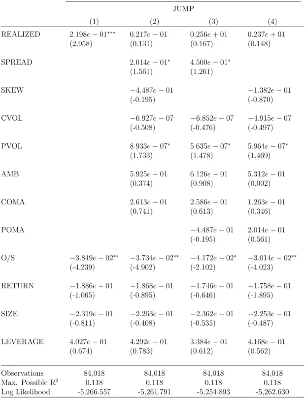
Table 4.5 documents the result of univariate and multivariate regressions for JUMP variable. Univariate model, regression (1), is significant at 1% level with a positive coefficient. It means that, the volatility in historical prices can predict whether there is going to be a large upward movement in stock prices or not. The sign of realized volatility variable in Table 4.6 is also significantly positive at 1% level. This result denotes a warning that investors who use realized volatility for prediction should be careful interpreting their results. Because same sign indicates that realized volatility can forecast a large movement, yet it cannot forecast its direction. Rather, using implied volatility and volume measures gives the complete picture about future expectations. Regressions (3), (4), and (5) in both tables show that realized volatility lose its significance to other explanatory variables. Moreover, other variables have similar significance level as in the main results. Importantly, CVOL has a negative coefficent with significance levet al 10% while PVOL is positively significant at 5% level in CRASH regressions. This result provides further support for first and second hypotheses. Once again, options volumes’ signs do not support the third and forth hypotheses. However overall results are consistent throughout the thesis.

4.3 Robustness Check: Bear and Bull Market

My work’s objective is to analyze large stock price movements, i.e. crash and jump. These large movements are considered at the firm-level, but possible rea-son(s) behind these movements has not been discussed in this study. One reason for this is the scope of this study. In this thesis, I am not trying to explain why there is or is not a large movement in stock prices, but their predictability from options market perspective. However, it is important to check the e↵ect of finan-cial crisis on large stock price movements, because crises cause traders behave

Table 4.5: Robustness Check: With Realized Volatility

Dependent variable: JUMP

(1) (2) (3) (4)

REALIZED 2.198e 01⇤⇤⇤ 0.217e 01 0.256e + 01 0.237e + 01

(2.958) (0.131) (0.167) (0.148)

SPREAD 2.014e 01⇤ _{4.500e 01}⇤

(1.561) (1.261)

SKEW 4.487e 01 1.382e 01

(-0.195) (-0.870)

CVOL 6.927e 07. _{6.852e 07 4.915e 07}

(-0.508) (-0.476) (-0.497)

PVOL 8.933e 07⇤ _{5.635e 07}⇤ _{5.964e 07}⇤

(1.733) (1.478) (1.469)

AMB 5.925e 01 6.126e 01 5.312e 01

(0.374) (0.908) (0.002)

COMA 2.613e 01 2.586e 01 1.263e 01

(0.741) (0.613) (0.346)

POMA 4.487e 01 2.014e 01

(-0.195) (0.561)

O/S 3.849e 02⇤⇤ _{3.734e 02}⇤⇤ _{4.172e 02}⇤ _{3.014e 02}⇤⇤

(-4.239) (-4.902) (-2.102) (-4.023)

RETURN 1.886e 01 1.868e 01 1.746e 01 1.758e 01

(-1.065) (-0.895) (-0.646) (-1.895)

SIZE 2.319e 01 2.263e 01 2.362e 01 2.253e 01

(-0.811) (-0.408) (-0.535) (-0.487)

LEVERAGE 4.027e 01 4.292e 01 3.384e 01 4.168e 01

(0.674) (0.783) (0.612) (0.562)

Observations 84,018 84,018 84,018 84,018

Max. Possible R2 _{0.118 0.118 0.118 0.118}

Log Likelihood -5,266.557 -5,261.791 -5,254.893 -5,262.630

Table 4.6: Robustness Check: With Realized Volatility

Dependent variable: CRASH

(1) (2) (3) (4)

REALIZED 1.983e 01⇤⇤⇤ _{0.819e 01 0.748e + 01 0.849e 01}

(1.676) (0.684) (0.476) (0.792)

SPREAD 1.068e 03 1.205e 01⇤⇤⇤

(-0.003) (-1.203)

SKEW 1.204e 01⇤⇤ _{1.205e 01}⇤⇤⇤

(3.084) (5.203)

CVOL 7.163e 07⇤ _{7.146e 07}⇤ _{7.219e 07}⇤

(-1.824) (-1.913) (-2.105)

PVOL 1.199e 06⇤⇤ _{1.532e 06}⇤⇤ _{1.452e 06}⇤⇤

(4.424) (4.418) (4.613)

AMB 3.382e 014 4.693e 01 4.558e 01

(-0.668) (-0.142) (-0.248)

COMA 1.658e 01⇤⇤⇤ _{1.785e 01}⇤⇤⇤ _{1.713e 01}⇤⇤⇤

(-3.870) (-4.070) (-3.912)

POMA 1.204e 02⇤⇤ _{1.068e 03}

(3.084) (-0.003)

O/S 3.092e 02⇤⇤ _{3.394e 02}⇤⇤ _{3.022e 02}⇤⇤ _{3.382e 02}⇤⇤

(-4.093) (-4.160) (-4.724) (-4.393)

RETURN 2.778e 01 3.074e 01 2.692e 01 3.374e 01

(-1.774) ( -1.952) ( -1.485) ( -1.874)

SIZE 1.386e 01 1.311e 01 1.457e 01 1.231e 01

(0.248) (0.072) (0.365) (-0.982)

LEVERAGE 2.116e 01 1.991e 01 1.986e 01 1.892e 01

(-0.683) (-0.641) (-0.635) (-0.583)

Observations 84,018 84,018 84,018 84,018

Max. Possible R2 _{0.118 0.118 0.118 0.118}

Log Likelihood -5,266.557 -5,261.791 -5,254.893 -5,262.630

di↵erently than normal times. Therefore, in those periods, the significance that I capture can very well be caused by this wide range behavior di↵erences not the firm’s specific feature. For example Guiso et al. (2013) find that after 2008 crisis investors risk aversion level increase chiefly and this leads investors to get out from stock market. I should show that this is not the case. This robustness check is to document that the results from main regressions hold in crises periods as well. Since I am interested in both up and down movement of stock prices, I analyze bull2 _{market period as well as bear}3 _{market period. To test my}

hypothe-ses, I divide the full sample into two sub-periods. I choose the bull market as the period between 2001 and 2007 which corresponds to the period after the dotcom bubble. I choose the most recent banking crisis in US as the bear market. The period expands from the last two quarters of 2007 to at the end of 2009. I regress sub-sample models for each dependent variable.

2_{Bull market is a name for a stock market behavior when it is appreciating.} 3_{Bear market refers to the declining period of stock markets.}

One explanation for insignificant PVOL in Table 4.7 could be that investors be-come less risk averse in more positive times which supports ? findings. Since they are optimistic about the future, they may lower their put options positions, hence a significant decrease in out options volume. Results are more pronounced in bear market. In contrast to bull market, traders in bear market become more conservative about the preservation of their status hence they increase their op-tions posiop-tions. While CVOL stays at similar level, PVOL has 1% significance. This also confirms that investors use put volumes in bad times or at least when their expectation about the future is pessimistic. Especially, the variables with OTM-put in their calculations have higher significance in bear market if the de-pendent variables is CRASH, Table 4.10. On the other hand, results in Table 4.8 is similar to main results. It is valid for also JUMP variable in bear market, Table 4.9. Therefore, the investors in bear and bull market behave alike when the expectation is about upward and downward movement of stock prices respec-tively. However; my results contradict with Hwang & Satchell (2010). Hwang & Satchell (2010) show that investors act in a more loss averse way in bull markets compared to bear markets. The di↵erence between this thesis and the paper is that I use options market rather than stock market data. There has been no study which works on investor sentiment in options market. Although I can-not compare the conflicting results, this would be a good opportunity to start a sentiment analysis in options market.

Main point of these robustness checks is to show the links between dependent and independent variables are quite robust before a firm-level crash or jump. However, behavior of investors changes before jumps; therefore I refute H3 and H4, while robustness checks support H1 and H2.

T a bl e 4 .7 : R ob u st n es s C h ec k : B UL L M AR K E T (JUL Y 20 02 -S E P T E M B E R 20 07 ) D ep endent var iable: JUM P (1) (2) (3) (4) (5) (6) (7) (8) P R E AD 3. 867 e 01 ⇤⇤ 3. 146 e 01 ⇤ 3. 579 e 01 ⇤ (2.153) (1.583) (1.671) KEW 2. 165 e 01 ⇤⇤ 3. 836 e 01 3. 518 e 01 (-3.758) (-0.736) (0.024) OL 0. 182 e 05 0. 345 e 05 ⇤ 1. 085 (-0.803) (-1.1 15) (-0.303) OL 1. 052 e 06 ⇤⇤ 1. 958 e 06 ⇤⇤ 1. 538 e 06 ⇤⇤ (4.813) (4.392) (4.346) B 2. 132 e 01 ⇤⇤⇤ 2. 538 e 01 ⇤⇤ 2. 071 e 01 ⇤⇤ 2. 108 e 01 ⇤⇤ (4.022) (3.016) (3.298) (3.829) 3. 146 01 ⇤⇤⇤ 3. 493 e 01 ⇤⇤ 3. 215 e 01 ⇤⇤ 2. 056 e 01 ⇤ (-6.138) (-5.912) (-5.356) (-3.328) 5. 312 e 02 5. 446 e 02 5. 335 e 02 (-0.345) (-0.146) (-0.218) 2. 348 e 02 ⇤ 2. 932 e 02 ⇤ 3. 823 e 02 ⇤ 2. 210 e 02 ⇤ 4. 340 e 02 ⇤ 4. 752 e 02 ⇤ 3. 223 e 02 ⇤ 3. 902 e 02 ⇤⇤ (-3.248) (-2.953) (-3.752) (-2.834) (-4.363) (-4.827) (-3.392) (-3.392) E T UR N 2. 396 e 01 3. 984 e 02 2. 094 e 01 3. 095 e 01 2. 583 e 02 4. 238 e 01 2. 784 e 01 2. 117 e 01 (-1.097) (-0.895) (-1.007) (-0.256) (-0.846) (-0.254) (-0.335) (-0 .456) IZE 1. 947 e 01 1. 725 e 01 1. 348 e 01 1. 908 e 01 1. 095 e 01 1. 803 e 01 1. 458 e 01 1. 987 e 02 (-0.480) (-0.268) (-0.537) (-0.182) (-0.547) (-0.478) (-0.485) (-0 .045) E VE R A G E 6. 047 e 01 7. 895 e 01 7. 988 e 01 6. 405 e 01 6. 397 e 01 6. 489 e 02 8. 983 e 01 7. 046 e 01 (0.785) (0.354) (0.240) (0.408) (0.256) (0.504) (0.130) (0.898) ations 84,018 84,018 84,018 84,018 84,018 84,018 84,018 . P ossi b le R 2 0.154 0.154 0.154 0.1 54 0.154 0.154 0.154 Lik eliho o d -6,864.180 -6,864.464 -6,860.49 5 -6,856.057 -6,867.729 -6,698.816 -6,685.073 ⇤p < 0.1; ⇤⇤p < 0.05; ⇤⇤⇤ p < 0.01

T a bl e 4 .8 : R ob u st n es s C h ec k : B UL L M AR K E T (JUL Y 20 02 -S E P T E M B E R 20 07 ) D ep endent var iable: C R AS H (1) (2) (3) (4) (5) (6) (7) (8) S P R E AD 4. 852 e 01 ⇤⇤ 2. 143 e 01 1. 455 e 01 ⇤⇤⇤ (-3.841) (-1.532) (-5.6 73) S KEW 4. 143 e 02 ⇤⇤ 1. 316 e 02 ⇤⇤ 1. 753 e 02 ⇤⇤⇤ (4.376) (4.872) (6.488) CV OL 9. 145 e 07 ⇤ 9. 777 e 07 ⇤ 9. 176 e 07 ⇤ (-2.379) (-2.635) (-2.435) PV OL 1. 212 e 07 ⇤⇤ 2. 286 e 06 ⇤⇤ 1. 185 e 06 ⇤⇤ (3.723) (5.129) (3.642) AM B 1. 135 e 01 ⇤⇤ 5. 286 e 01 5. 807 e 01 6. 935 e 01 (-3.071) (-0 .127) (-0.345) (-0.653) COMA 1. 314 e 01 ⇤⇤⇤ 1. 629 e 01 ⇤⇤ 1. 269 e 01 ⇤⇤ 1. 093 e 01 ⇤⇤ (-5.516) (-4.325) (-4.256) (-4.100) POMA 5. 113 e 02 ⇤⇤ 1. 456 e 02 0. 918 e 02 (3.015) (0.716) (-0.128) O/S 3. 092 e 02 ⇤ 3. 230 e 02 ⇤ 1. 230 e 02 ⇤ 2. 239 e 02 ⇤ 2. 839 e 02 ⇤ 3. 519 e 02 ⇤ 2. 471 e 02 ⇤ 2. 405 e 02 ⇤⇤ (3.302) (3.731) (3.530) (4.612) (4.202) (4.340) (4.204) (4.337) R E T UR N 2. 657 e 01 2. 384 e 01 2. 942 e 01 2. 953 e 01 2. 135 e 01 2. 842 e 01 2. 473 e 01 2. 853 e 01 (-0.864) (-0.305) (-0.030) (-0.0 67) (-0.107) (-0.452) (-0.673) (-0.234) S IZE 1. 207 e 01 1. 210 e 01 1. 744 e 01 1. 238 e 01 1. 417 e 01 1. 645 e 01 1. 948 e 01 1. 486 e 01 (0.384) (0.982) (0.991) (0.404) (0.103) (0.775) (0.353) (0.610) L E VE R A G E 1. 470 e 01 1. 357 e 02 1. 579 e 02 1. 691 e 01 1. 335 e 01 1. 734 e 01 1. 357 e 01 1. 524 e 01 (0.952) (0.846) (0.655) (0.559) (0.701) (0.735) (0.459) (0.901) Observ ations 84,018 84,018 84,018 84,018 84,018 84,018 84,018 Max . P ossi b le R 2 0.118 0.118 0.118 0.118 0.118 0.118 0.118 Log Lik eliho o d -5,268.687 -5,26 1.791 -5,254.893 -5,262.630 -5,270.988 -5,176.541 -5,144.329 N ote: ⇤p < 0.1; ⇤⇤p < 0.05; ⇤⇤⇤ p < 0.01

T a bl e 4 .9 : R ob u st n es s C h ec k : B E AR M AR K E T (O C T O B E R 20 07 -D E C E M B E R 20 09 ) D ep endent var iable: JUM P (1) (2) (3) (4) (5) (6) (7) (8) P R E AD 4. 385 e 01 ⇤⇤ 2. 116 e 01 2. 795 e 01 (2.152) (0.345) (0.451) KEW 1. 142 e 01 2. 105 e 01 3. 916 e 01 (-0.557) (-0.431) (-1.547) OL 1. 833 e 07 1. 642 e 06 ⇤ 1. 711 e 07 (-2.101) (-1.472) (-1.301) OL 2. 175 e 07 ⇤⇤ 2. 199 e 06 ⇤⇤ 2. 728 e 06 ⇤ (3 .7 47 ) (4 .0 85 ) (4 .2 11 ) B 2. 486 e 02 ⇤⇤⇤ 6. 956 e 01 5. 453 e 01 6. 135 e 01 (-2.167) (-1.326) (-1.485) (-1.653) 1. 512 e 01 2. 488 e 01 2. 629 e 01 2. 873 e 01 (-0.984) (-0.813) (-0.745) (-0 .132) 7. 396 e 022 7. 438 e 02 7. 135 e 02 (-0.218) (-0.119) (-0.132) 4. 186 e 02 ⇤ 3. 250 e 02 ⇤ 5. 421 e 02 ⇤ 5. 394 e 02 ⇤ 4. 735 e 02 ⇤ 4. 599 e 02 ⇤ 4. 290 e 02 ⇤ 4. 694 e 02 ⇤⇤ (-3.788) (-4.227) (-3.885) (-3.569) (-5.128) (-4.842) (-3.212) (-3.7 05) E T UR N 3. 856 e 02 2. 172 e 02 3. 043 e 02 4. 220 e 02 4. 360 e 02 1. 057 e 02 4. 227 e 02 4. 973 e 02 (-0.458) (-0.123) (-0.149) (-0.576) (-0.623) (-0.031) (-0.028) (-0.0 59) IZE 1. 698 e 02 1. 176 e 02 1. 486 e 03 1. 569 e 02 1. 705 e 02 1. 227 e 02 1. 149 e 02 1. 103 e 02 (-0.642) (-0.353) (-0.050) (-0.260) (-0.376) (-0.125) (-0.395) (-0.8 63) E VE R A G E 7. 776 e 02 6. 513 e 01 5. 598 e 02 5. 812 e 01 5. 086 e 01 6. 469 e 02 8. 377 e 01 7. 158 e 01 (0.022) (0.023) (0.413) (0.425 ) (0.916) (0.774) (0.575) (0.993) ations 84,018 84,018 84,018 84,018 84,018 84,018 84,018 . P ossi b le R 2 0.154 0.154 0.154 0.154 0.154 0.154 0.154 Lik eliho o d -6,864.180 -6,864.464 -6,860.49 5 -6,856.057 -6,867.729 -6,698.816 -6,685.073 ⇤p < 0.1; ⇤⇤p < 0.05; ⇤⇤⇤ p < 0.01