Shahrood University of Technology Iranian Society of Mining Engineering (IRSME)
(JME)
journal homepage: www.jme.shahroodut.ac.ir
Vol. 11, No. 1, 2020, 1-20.
DOI: 10.22044/jme.2020.8947.1781
A New Stability Approach Using Probabilistic Profile along Direction
of Excavation
A. Turanboy1*, E. Ülker2 and C.B. Küçüksütçü3
1. Department of Mining Engineering, Necmettim Erbakan University, Seydişehir Ahmet Cengiz Engineering University, Konya, Turkey 2. Department of Computer Engineering, Faculty of Engineering and Natural Sciences, Konya Technical University, Konya, Turkey
3. Bay E Information Education Consultant and Information, Selcuk University, Konya, Turkey
Received 25 September 2019; received in revised form 20 January 2020; accepted 22 January 2020 Keywords
Wedge failures
Data analyses
Visual representations
Monte Carlo simulation
Abstract
Estimation of the possible instability that may be encountered in the excavation slope(s) during the planning and application steps of the rock excavation processes is an important issue in geoengineering. In this paper, a modelling method is presented for assessing the probability of wedge failure involving new permanent or temporary slope(s) along the planned excavation direction. The geostructural rock slopes including wedge blocks are determined geometrically in the first step. Here, a structural data analysis system that includes a series of filterings, sortings, and linear equations used to reveal the necessary geometric conditions for the wedge form is developed and used. The second step involves the 3D visualization and Factor of Safety (FS) using the limit equilibrium analysis of wedges on both the actual and planned new excavation surfaces. The last step is the Monte Carlo simulation, which is used in assessing the instabilities on the actual and planned new excavation surfaces. These new slope surfaces that have not yet been excavated are called the virtual structures. As a result of this work, the mean and probabilistic FS variations in the planned excavation direction are obtained as profiles. We suggest the preliminary guidelines for the mean and probability of the wedge failure in the excavation direction. The model is tested on a motorway cut slope. The FS results obtained from the Monte Carlo simulation calculations are compared with the mean results and the changes are revealed with the reasons.
1. Introduction
The stability analysis of rock slopes is essential for a safe design of excavated slopes like open-pit mines and road cuts. The geometric properties of discontinuities play a decisive role in influencing these analyses. Piteau (1972) [1] has stated that the stability of rock slopes is determined principally by the structural discontinuities in the mass and not by the strength of the rock itself. Additionally, the stability of rock masses is commonly controlled by the presence of discontinuities at shallow depths (Hoek and Bray 1981) [2]. The analysis of rock slope stability consists of a series of processes. The first step is usually the kinematic
analysis related to the presence of discontinuities and their orientations to determine the instability of the slope. The stereo-graphic projections are generally used in this process. If the results indicate that the slope is clearly stable, no further analysis such as limit equilibrium or probabilistic analysis is performed. If any kinematically possible failure mode is determined, a limit-equilibrium stability analysis is required as the second step to compare the forces resisting failure with the forces causing failure. In this deterministic analysis, all the input parameters are applied as fixed values despite the fact that all parameters
show a degree of variability, and a fixed factor of safety (FS) is obtained as a result. On the other hand, rock masses are complex structures owing to the geometry of their discontinuities. Moreover, the characterization of rock masses is subject to uncertainties due to the limited data that is gathered during field surveys. Due to the complex geometry of the rock blocks and the associated uncertainties concerning the physical and mechanical parameters for solving the stability problems of rock slopes, statistical approaches are necessary [3, 4]. Therefore, the probability-based methods have been of great interest in slope stability assessments for a long time. Being one of the most basic statistical methods, Monte Carlo simulation (MCS) has the capability of solving a broad range of stability problems and has been used by several researchers to evaluate the rock slope stability [5-18]. The main disadvantage of this technique is the extensive computational time, which increases substantially in the numerical analyses [19].
Investigating all the discontinuities and blocks in rock slopes is extremely difficult. Moreover, discontinuities are generally randomly distributed in rock masses [20]. Hence, any geometric characterization of a rock mass must be performed based on the theory of statistics and probability. In addition, most rock failures occur during slope excavation [2]. Additionally, wedge failure is a common and the most observed failure mode, and is primarily controlled by the orientation and spacing of discontinuity surfaces with respect to the slope surfaces [2, 21, 22]. For this reason, it is very important to predict the instability respond to wedge blocks on new slopes to be excavated such as the extension of motorway cuts and open-pit bench excavation applications. Until now, the kinematic, kinetic, and statistical evaluations on instability of rock slopes have been made in the form of representing the entire rock masses using samples only from a single structure (the actual slope). However, the rock excavation applications are dynamic processes, and adverse conditions may be encountered during the excavation in temporary multi-step slopes. Therefore, a statistical failure analysis based on new excavation surfaces is a useful tool for predicting failures that may also be encountered in the excavation direction. There are three types of 3D models in the literature [23]: the wireframe, surface, and solid models. The wireframe models are preferred
when the volume and space occupied are not important. The solid models are used when the mass is completely homogeneous, and it is sufficient to model it with basic primitives [24-30]. The surface models are used if the shape of the surface matters [31, 32]. For example, the B-spline surfaces are such a modelling tool. Each plane on the surface is considered as a surface patch, and the interpolation methods are used. Contrary to the classic modeling approaches, the spatial interpolation methods incorporate information about the geographic position of sample points [23].
In the developed software, solid modelling is preferred beause the whole rock mass is analyzed rather than the large and small indentations on the surface of rock mass. Due to the computer science and software requirements, certain rules have been introduced in the models to be produced. The slope surfaces are assumed to be planar. Our model was constructed based on the geometry of tetrahedron wedge blocks, which form only on two cross-discontinuities and along the slope crest. These wedges may not be formed perpendicular to the slope surface. In addition, the authors focus on a new methodology for the generation of Virtual Structures (VSs), which are behind the actual excavation surface, and the evaluation of the wedges on these structures. In the developed model, each VS is treated as two surfaces: the excavation and upper slope surface on which wedges are formed. In addition, a probabilistic variation in the FS values in the excavation direction was obtained. All the statistical evaluations were performed by MCS, which is widely used for rock stability calculations.
2. Wedge Geometry and failure mechanism
The presence of the wedge form can be easily determined using the stereonet technique, and a kinematic stability analysis of wedge is based on the Markland’s Test [33]. Figures 1a, 1b, and 1c show the commonly used basic geometric dimensions of a wedge block, which are used to calculate FS according to Hoek and Bray (1981) [2]. A wedge failure may occur under the following conditions: i) the wedge block must be formed when two discontinuities (joints, bedding planes, foliations, etc.) intersect diagonally within rock slopes; ii) the dip of intersection line of two discontinuities of the wedge must be in the same direction as the slope face; iii) the dip of the slope must be greater
than the dip of the line of the intersection of the wedge-forming discontinuity surface; vi) the line of intersection must be greater than the interior friction angle, and the intersection points of wedge must be daylighted on the slope face; and v) the dip of the line of intersection must be such that the strengths of the two surfaces are reached [2, 34]. Besides, according to Wyllie and Mah (2004) [35], if the dip directions of the two surfaces lie outside the included angle between i (trend of the line of
intersection) and s (dip direction of the face),
the wedge will slide on both surfaces (Figure 1d); however, if the dip direction of one plane lies within the included angle between i and s,
the wedge will slide only on that plane, and in this case, the planar slip conditions will be valid. Zheng et al. 2016 [36] have classified these two types as a standard wedge and an overlying wedge, respectively. Turanboy 2016 [37] has proposed a 2D wedge shape classification system according to all their possible geometries, the boundary elements (edges, corners, and angles of the wedge blocks), and their relative positions against each other using linear relations. In this classification system, the standard and overlying wedge forms are presented together systematically. The proposed model considers standard wedges with a sliding potential on two diagonal discontinuous planes.
The LE approach, which is used in designing engineered slopes, considers the relationship between the strength or the resisting force and the demanding stress or the disturbing force [2]. Many researchers [2, 21, 33, 35, 38-52] have studied and presented in detail the mechanisms by which wedge blocks slide on rock slopes on this basic principle. In addition, if wedge failure is analysed assuming that sliding is resisted only
by friction and there is no contribution of cohesion, FS can be computed by Equations 1 to 6, presented by Hoek and Bray 1981 [2]. The solution was also adopted to our model.
𝐹𝑆 =(𝑅𝐴+ 𝑅𝐵)𝑡𝑎𝑛𝜙
𝑊𝑠𝑖𝑛 (1)
where RA and RB are the normal reactions
provided by two intersecting discontinuities, W is the weight of the wedge, ϕ is the friction angle of the planes, and is the angle between the intersection line and the horizontal axis. The forces RA and RB are found by the following
relations: 𝑅𝐴𝑠𝑖𝑛(− 1 2) = 𝑅𝐵𝑠𝑖𝑛(+ 1 2) (2) 𝑅𝐴𝑐𝑜𝑠 (− 1 2) + 𝑅𝐵𝑐𝑜𝑠 (+ 1 2) = 𝑊𝑐𝑜𝑠 (3)
where the angles and β are measured on the great circle (Figure 1c). In order to meet the condition for equilibrium, the normal components of the reactions should be equal. The values for RA and RB can be found by
solving Equations 4, 5, and 6 as:
𝑅𝐴+ 𝑅𝐵=
𝑊𝑐𝑜𝑠 𝑠𝑖𝑛
sin (⁄ )2 (4)
cos sin tan . sin / 2 sin FS or, (5) 𝐹𝑆 = 𝑠𝑖𝑛 sin (⁄ )2 ∙ 𝑡𝑎𝑛𝜙 𝑡𝑎𝑛 (6) 𝐹𝑆𝑤= 𝐾 𝐹𝑆𝑝 (7)
where FSw is FS of the wedge and FSp is the FS of the plane failure. K is the wedge factor, which depends upon the included angle of the wedge
and the angle of tilt of the wedge. Figure 1 shows the detailed geometry and conditions of the wedge failure.
Figure 1. Geometric conditions of a wedge failure that are used in calculating FS: (a) cross-section of a wedge showing the resolution of the wedge weight W; (b) view of a wedge face showing the definitions of angles β, /2, and θ, and the reactions on sliding planes RA and RB; (c) stereo-net showing the angles β and ε/2 (after Hoek and Bray, 1981 [2]); (d) the kinematic condition associated with the wedge has two sliding
3. Monte Carlo Analysis in Wedge stability
In the conventional methods, the failure is assumed to occur when FS is less than 1. Rather than basing the engineering design decisions on a single calculated FS, the probabilistic approaches associated with a particular model give a more rational assessment [2]. Monte Carlo simulation (MCS) performs risk analysis by building models of the possible results by substituting a range of values for a probability distribution for any factor that has an inherent uncertainty since the rock wedge stability analysis often includes many uncertainties due to the inadequacy of the information obtained during site characterization as well as the variability and the measurement errors that are inherent in the measurement of the geological and geomechanical parameters [50, 53]. Carrying out the probabilistic slope stability analysis with MCS, which allows for a systematic and quantitative treatment of these uncertainties, has become a topic of increasing interest for rock slope engineering. MCS can be applied to the problems that are very difficult to solve with the analytical methods (Giani, 1992) [54]. Even Feng and Lajtai (1998) [55] have stated that MCS is most convenient among the probabilistic analyses. MCS generates a large quantity of random numbers varying between 0 and 1. Such curves can be histograms that are drawn according to the experimental and field data. These numbers are used to generate the variables of the problem in a way that fits the assumed probability distribution curves. Several researchers [15, 16, 18, 56, 57] have
also successfully implemented the method using commercial softwares such as SWEDGE [58].
In the modelling study, MCS is used to be linked to LE analyses given in Equation 6 and its parameters (𝜙, β, /2, and θ) are considered as uncertainties.
4. Methodology
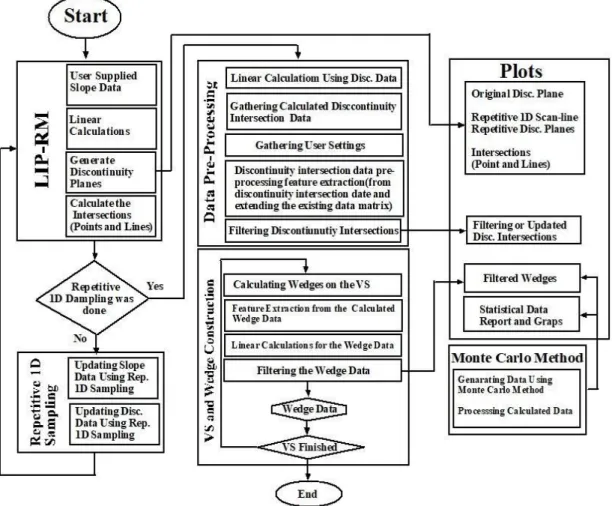
The model is an integrated system with tightly connected modules. The process consists of the construction of VSs with wedge structures in the direction of excavation, identification of wedge failure probabilities for each VS, and plotting the variation in these probabilities. In order to facilitate explanation, the system is divided into different sub-components. For this reason, the study was implemented in four basic steps: i. generation of the entire 3D rock mass model using LIP-RM, which is a software programme already developed by the authors (Turanboy and Ülker, 2008) [59], ii. Data processing for expanding the actual scan-line measure to the left and right sides and generating the wedge, iii. Construction of VSs with wedge form using the rules of linear algebra and computational geometry, and iv. Probability calculation for the actual and generated VSs. Finally, the change in the mean and probabilistic FS in the direction of excavation using 2D line charts was presented. The pseudo-code of the generated algorithm can be presented as below.
Step 1 Running LIP-RM
Create the Information System Table and fill the scan-line survey. Calculate the discontinuity planes.
Calculate the intersection points and lines of all discontinuities together. Save Slope Data and Discontinuity Data to Database.
Step 2 Data Pre-processing
Expand the actual scan-line measure to the left and right sides (Repetitive 1D Sampling). Update the new discontinuity and calculate the intersections.
Select the actual rock slope and generate the intersection lines. Filter the cross ones (discontinuity planes).
Generate the wedges
Step 3 VS Construction
Take the number of VSs from the user. Calculate wedges on VS.
Do Each VS.
Calculate the β, /2, θ, and 𝜙 parameters of the Selected Wedges on VS Save Data for using the Monte Carlo Method.
Run the MCS Method. Plot wedges on the VS crest. Loop
Figure 2 shows a flowchart of the developed algorithm, in which the connecting lines and
directional arrows are numbered to simplify the presentation.
Figure 2. Flowchart summarizing LIP-RM, data processing, VS and wedge construction, and MCS method.
4.1. Field survey and initial dataset
According to Priest and Hudson (1981) [60] and Priest (1993) [61], the first step of the model involves obtaining the raw (initial) input data using a scan-line survey. In the model, the discontinuity features such as the dip, dip direction and spacing defined by ISRM (1981) [62] and slope orientation information are used. Using these input data, new computable data is obtained within the model process. A table called the Information System Table (IST) was created as the first input data for the model. Table 1 shows an example of IST. This table
contains information about the geometric properties of discontinuities and slope separately. All the secondary data used in the model is calculated from these data.
All inputs and calculated values are stored in a database to be accessed at every step of the model. The calculated values are based on the assumption that claiming wedges are formed only on the free structures. The conditions under which any three or four discontinuities can form a tetrahedron in the rock mass are not considered.
Table 1. An example of IST data.
Discontinuity/Outcrop ID Dip (degree) Dip dir. (degree) Cumulative spacing (m) Outcrop D1 80 20 185 24 - 5 D2 68 88 10 .. .. .. Dn 89 340 150
4.2. Generation of overall 3D rock mass model and LIP-RM summary
The same initial assumptions in the original version of LIP-RM were made in the design of the model: i. all the discontinuity surfaces were assumed to be perfectly planar; ii. The discontinuity surfaces were assumed to extend entirely through a Representative Cuboidal Prism (RCP), and iii. all discontinuities were randomly oriented. These assumptions were the already used approaches such as the block
theory [66] to identify the removable blocks and the Discrete Fracture Network (DFN) modelling [64] to represent the geometry of the existing discontinuities. In addition, the LIP-RM software package was adopted to develop the model; it represents a 3D discontinuity network. These modifications are related to the construction of new VSs and repetitive 1D sampling of modelling rock mass, as explained in detail below. The pseudo-code of LIP-RM is presented below:
Parameters: scan-line height, selected dimensions of the cuboids, outcrop orientation.
Input of the measured values used in the survey method (dip, dip direction, cumulative space, points of the discontinuity) to Information System Tables
Do all discontinuities
Classify processes of every discontinuity Generate the discontinuity plane
If the discontinuity plane exceeds the cuboid, then prune the discontinuity surface Save the discontinuity plane to database
Loop
Limit = number of discontinuities For i = 1 to limit-1
Read Plane of the Discontinuity (#i) For j = i + 1 to Limit
Read Plane of the Discontinuity (#j)
Calculate the intersection points between the discontinuity planes (#i and #j) If there is an intersection between #i and #j, then
calculate the intersection points save the intersection points to database
End if
Next j Next i
Visualize the rock mass on the screen
In the LIP-RM software, the building of the (information system) table includes recording the data in the first phase. For calculation of any discontinuity plane, four intersection points were computed on the cuboid edges. Then the discontinuity plane with these assistant points was generated. Moreover, LIP-RM could find the intersection point for any two or more discontinuity planes and the corresponding intersection lines. Thus the images of all discontinuity planes and the rock block were simulated. The isometric presentation is preferred in the LIP-RM software, which is named as a “linear isometric projection of rock mass. The input data of LIP-RM is the discontinuity geometric properties such as dip, dip direction and spacing on the rocky outcrop in the form of an information system. The output is a simulation model consisting of the rock mass structure and a database. The key
components of the LIP-RM model are (i) classification of orientations of the discontinuity planes and outcrop according to the north (ii) mathematical definition of the discontinuity planes, and (iii) isometric transformation and projection of the rock structure including the discontinuity planes, their intersection with each other, and the created blocks bounded by discontinuity planes and/or free surfaces [59].
LIP-RM uses the parametric equations to define the co-ordinates of the intersections of discontinuities with each other and the corner points of an RCP (whose dimensions can be selected by the user), and draws discontinuity traces on the RCP structures within a hierarchy to create a 3D discontinuity network model of the whole rock mass. Co-ordinates of the intersections between pairs of discontinuities and between discontinuities and the edges of the
prism as well as the spatial data on discontinuities are inputs to the newly developed model. In addition, the results obtained from LIP-RM is useful in interpreting the input data and the final results.
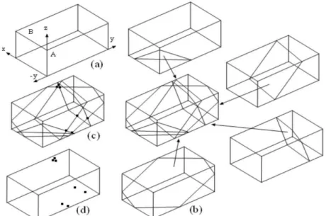
Figure 3a shows the first initial structure to be modelled according to IST. Surfaces A and B are the excavation and upper slope surfaces, respectively. Each discontinuity on this surface was handled individually, and the discontinuity plane was obtained as shown in Figure 3b by
passing straight lines through the prism edges. The LIP-RM software finds the intersections of discontinuities on six faces of RCP. Here, the possible discontinuity planes with a maximum of six and a minimum of three edges and corners could be constructed. Then co-ordinates of the intersections were recorded in the database. Figure 3c shows the intersections on structures A and B, respectively, together with the discontinuity surfaces. Figure 3d shows the intersection points on surfaces A and B.
Figure 3. Basic steps of LIP-RM: (a) the first initial structure (RCP); (b) intersections of discontinuities on six faces of RCP; (c) intersections (on surfaces A and B) together with the discontinuity surfaces; (d) intersection points (on structures A and B). Note that surfaces A and B correspond to the excavation and
upper slope surfaces, respectively.
The initial data in IST contains information on the properties of orientation(s) of the actual slope (s): the number (Id) denoting the current slope as well as the dimensions and corner co-ordinates of the slope along the x-, y-, and z-axes. The information on discontinuities (i.e. information calculated by LIP-RM to determine 2D polygons) represents the visible surfaces of the tetrahedrons on the excavation and upper slope surfaces. The polygons are identified as wedge forms on the actual surface (Figure 4). The information in this step includes the specific unique number of the slope, (Id-number) of the discontinuity, and the x, y, and z co-ordinates of up to six calculated corners of a polygon. Figure 3d shows the information on the intersection points that are calculated by LIP-RM.
The surfaces A and B and the intersection points on them are significant when combined with the initial assumptions to form wedges. Within the
boundaries of the prism, the model produces a wedge polygon with two diagonal discontinuities that can intersect with each other on surfaces A and B (Figure 4).
4.3. Construction of VSs
The LIP-RM software package was modified to show VSs with wedge forms on them. VSs may resemble the geological cross-sections that are created by several survey methods such as scan-lines or well logs. Furthermore, VSs are used probabilistically to evaluate the instabilities in response to the wedge failure. Although the geological cross-sections are 2D, two surfaces were considered in the model.
These two surfaces are considered as new excavation and upper slope surfaces for any excavation step or planning phase, where the excavating equipment is worked. New excavation and upper slope surfaces are parallel and perpendicular to the excavation direction,
respectively, and discontinuity traces are cloned these newly created surfaces without changing their spatial positions, which are measured on the actual structure at this step. Therefore, on each surface, different shapes and volumes of wedges are formed depending on the spatial properties (dip and dip direction) of discontinuities and the properties defined in Equation 6.
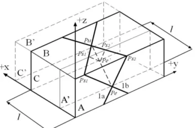
Initially, the authors considered a new excavation surface (Surface A) that was parallel to and behind the actual slope surface (surface A) (Figure 4). Then it was detected whether or not a new wedge was formed on the new slope surface. If neither of the straight lines |Pu Pe|, |Pu Ps1|, and |Pu Ps2| intersected the new surface, then no wedge was formed on this surface. If anything, the intersection points Pe', Ps1' and Ps2 and, subsequently, the straight lines |Pu Pe|, |Pu Ps1|, and |Pu Ps2| were obtained using the linear interpolation and the triangle
similarity rules with no additional calculation. Thus the wedge polygons formed on the new surface (A), which were parallel to the front surface (A) of RCP. A similar process was applied on the upper slope surface (B) to obtain the second triangle component of the tetrahedron. In contrast, the process of assigning a wedge form was realized according to the dip direction of the slope, the dip direction of the intersected surfaces, and the calculated trend of the line of intersection (Figure 1d). Those that did not form tetrahedral structures were eliminated within the prism boundaries. In this case, the model only contained the wedges that were formed by the discontinuities that were defined by the measurement of the actual excavation surface. Note that wedge sliding on two surfaces (A and B) was taken into account in the model. In addition, the C surface was considered as the final surface to be excavated in the model (Figure 4).
Figure 4. Checking for existence of a wedge on a newly constructed surface (A). Note that l is the dimension of RCP in the +x-direction.
4.4. Repetitive 1D sampling of RCP
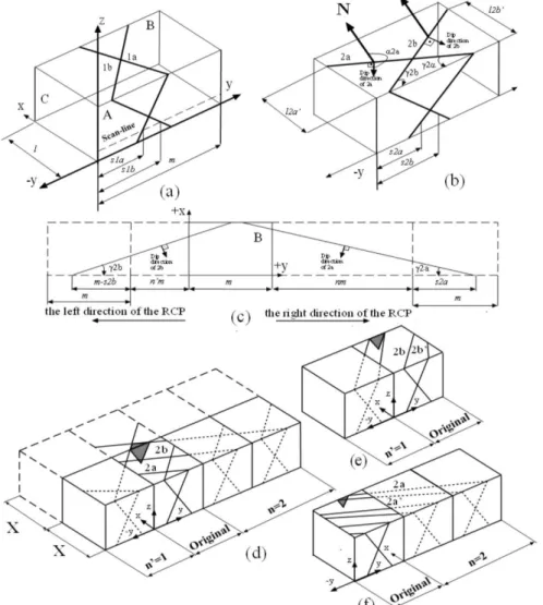
RCP can only contain the discontinuities that are recorded by a scan-line measurement. In order to overcome this problem, the original scan-line measurement is imaginatively extended in both the –y- and +y-directions, assuming that the original scan-line measurements are repetitive in these directions. Here, the purpose was to include the discontinuities that were outside the scan-line measurement but could be found in RCP. Initially, four main discontinuity orientation conditions were taken into consideration (Figures 5a and 5b). While the discontinuity types 1a and 1b can form a wedge on the actual structure and final VS (Figure 5a), the
discontinuity types 2a and 2b cannot form a wedge on the final VS (Figure 5b). This means that the scan-line measurement cannot provide sufficient data for modelling VS behind the actual slope.
For example, the standard wedge structures on the actual excavation structure (Figure 4 and 5a) would have been successively repetitious with the same spacing along the +x direction; however, only these rhombus-like structures were obtained. Hence, each VS had the same probability, and thus a uniform probability distribution.
For this approach, the following equation can be established for the +y-direction (Equation 8):
𝑡𝑎𝑛 ϒ
2𝑎=
𝑙−𝑙2𝑎𝑠2𝑎−𝑛 𝑚
,
(8)where according to Turanboy and Ülker (2008) [59], the ϒ angles (Figures 5a, 5b, and 5c) are described with reference to the dip direction of the discontinuity and s2a is the cumulative
spacing, m is the scan-line length, l is the dimension of RCP in the +x-direction, and l2a is
the intersection point between the related discontinuities and the upper edges of RCP in the +x-direction (these co-ordinates are obtained from the output data of LIP-RM). The number (n) of RCP that should be added to the +y-direction of the modelled RCP is given by:
𝑛 =(𝑙 − 𝑙2𝑎) − 𝑡𝑎𝑛ϒ2𝑎(𝑠2𝑎) 𝑚 𝑡𝑎𝑛ϒ2𝑎
(9)
Similarly, for the –y-direction (Equation. 9),
𝑡𝑎𝑛ϒ2𝑏=
𝑙 − 𝑙2𝑏
(𝑚 − 𝑠2𝑏 ) + 𝑛′𝑚
(10)
where the number (n) of RCP that should be added to the –y-direction of the modelled RCP is given by
𝑛′ =(𝑙 − 𝑙2𝑏) − 𝑡𝑎𝑛ϒ2𝑏(𝑠2𝑏) 𝑚 𝑡𝑎𝑛ϒ2𝑏
(11)
Figure 5c shows the plan view resulting from this approach.
The suggested procedure is applied to all of the discontinuities, and n and nprisms (rounded up to the nearest integer) should be added to the original RCP in the –y- and +y-directions. According to Equations. 9 and 11, if n = 2 and n= 1, then discontinuity of types 2a–2b (Figure 5d), 2b–2b (Figure 5e), and 2a–2a (Figure 5f) can also form wedges on the final VS.
Figure 5. Conditions on upper surface of the slope: Type 1a and 1b discontinuities that (a) can be modelled up to the final VS; (b) cannot be modelled up to the final VS. (c) plan diagram that explains the geometric parameters that are employed in calculating the numbers of RCPs that should be added to the right and left of the RCP. For example, when n = 2 and n = 1, wedges (grey) that may be formed on the excavation surfaces of the final VS by different types of discontinuities: (d) 2a–2b, (e) 2b–2b and (f) 2a–
In addition, according to the model, the upper slope surface (B) is shifted by the same amount(x) as surface A in the x-direction; Figure 5d).
Thus all the linear elements can be modelled within RCP. All the required parameters for kinetic admissibility can be obtained in this step as a datasheet, which is then used in the MCS step.
5. Application of suggested method
An experimental slope at approximately 120 km along the Konya–Antalya motorway wall in Turkey was chosen (Figure 6). In this region,
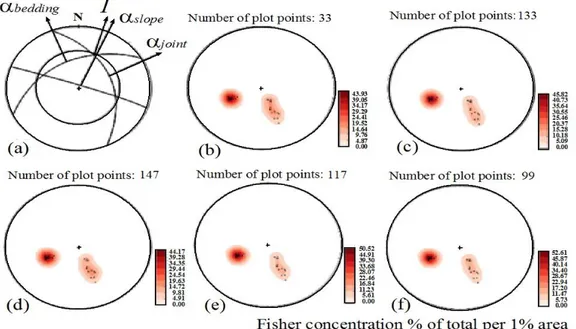
the main formations are composed of limestone and dolomite. The bedding planes and joints, which are approximately diagonal to each other, can be easily detected on the actual slope. According to Harrison and Hudson (1997) [34], a kinematic analysis is the first stage in a rock slope investigation. In this context, 33 discontinuities were obtained using the scan-line technique along the free structure (+y-direction), and two discontinuity sets were identified using the stereo-net analysis, following the procedures suggested by ISRM (1981) [63]. Figure 7 shows the structural and stereo-net analyses of the experimental slope.
Figure 6. Outcrop of modelled motorway slope. North direction and scan-line were drawn approximately.
Figure 7. Stereo-net analyses: (a) major sets of discontinuities within the experimental rock slope. Pole plots and their densities on A surface of (b) the experimental slope using the original scan-line measurement. After the modelling process: (c) the experimental slope; (d) 10th; (e) 20th, and (f) 30th (final
Since the discontinuities measured on the actual excavation surface were reflected on the other VSs without changing their spatial locations, their pole points were superimposed. Therefore, no visual changes could be observed in the scatter plots of the pole points on all surfaces. However, a partial change in their densities, according to the suggested approach, could be observed for Figures 7c (0th), 7d (10th), 7e (20th),
and 7f (30th (final VS)).
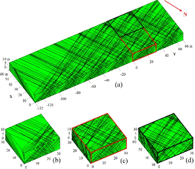
Figure 8a shows the extended 3D discontinuity block diagram. Here, n and n were determined to be 1 and 4, respectively, using Equations. 9 and 11. Figure 8b shows the constructed 3D discontinuity map, which was produced using LIP-RM in which only the scan-line measurements were used. The representation in Figure 8b was given in the original co-ordinate axes without regard to the repetitive 1D sampling of the RCP process. On the other hand, two 3D model parts that were obtained using the developed approaches can be seen in
Figure 8c (experimental slope after modelling processes) and Figure 8d (for the 30th final VS).
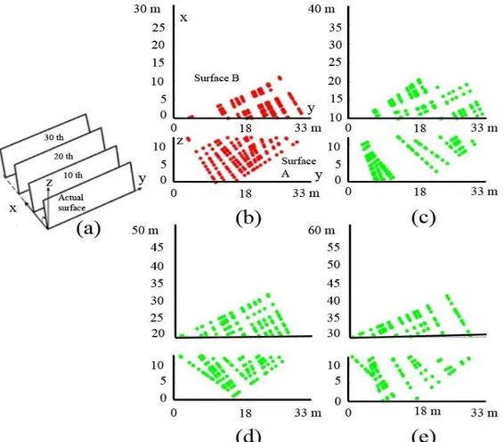
The 3D model part in Figure 8c is the basis for the next steps. VSs are selected at intervals of one m, perpendicular to the excavation surface. In other words, it was assumed that the excavation was to be carried out at intervals of one m. Thus 30 structures (VSs) including the current outcrop surface were modelled. (The first VS is the actual structure and is referred to as the initial VS in the model.) The VS intervals and the number can be selected by the user using the developed model. Figure 9a shows a schematic diagram of these 30 VS structures. (Only the excavation surfaces are shown to avoid complexity in the figure). The 2D scatter plots of the intersection points that formed wedges on the actual (0th), 10th, 20th, and final
VS are shown in Figures 9b–9e. In addition, Figure 10 shows the generated wedges along the crest of the slope for the sample VSs in Figure 9.
Figure 8. (a) Extended 3D discontinuity mapping. Constructed 3D discontinuity maps: (b) using only the scan-line measurements; (c) after modelling processes (thick red line); (d) corresponding to the 30th final
Figure 9. (a) Schematised existing actual excavation surface and the 10th, 20th, and final (30th) VSs, and the 2D scatter points of intersections that form wedges on the excavation (A) and upper slope (B) surfaces: (b) the 0th, (c) 10th, (d) 20th, and (e) final (30th) VSs. Note that the points on the actual slope are shown in red.
Figure 10. Generated wedges along the crest of the slope for (a) the actual (0th), (b) 10th, (c) 20th, and (d) th
One of the aims of this work was to investigate the effect of discontinuity orientations and their spatial variability using deterministic and probabilistic approaches based on wedge failure on newly defined VSs. First, a kinetic analysis was performed using the direct formula (Equation 6) with single fixed values (typically, mean values). According to Barton (1978) [65], it was assumed that the internal friction angle varied within the range of 340–400 for limestone
discontinuities. Thus a mean friction angle of 370 was assumed for all structures, and the
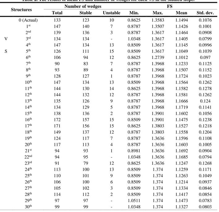
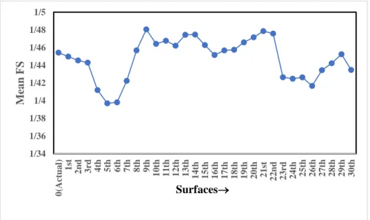
results of the mean FS as well as the number of wedges for each VS were obtained (Table 2). The mean FS results along the +x-direction are shown as a profile in Figure 11. Note that the +x-direction was considered as the excavation direction in both the kinetic and probabilistic analyses.
Table 2. The results of mean FS and number of wedges for each VS in the studied slope.
Structures Number of wedges FS
Total Stable Unstable Min. Max. Mean Std. dev.
0 (Actual) 133 123 10 0.8625 1.3583 1.1494 0.1076 1st 147 140 7 0.8787 1.3507 1.1426 0.1001 2nd 139 136 3 0.8787 1.3617 1.1464 0.0908 V 3rd 134 134 - 1.0348 1.3617 1.1405 0.0799 4th 147 134 13 0.8509 1.3617 1.1145 0.0996 S 5th 126 111 15 0.8509 1.3617 1.1049 0.1039 6th 106 94 12 0.8625 1.2739 1.1012 0.097 7th 90 83 7 0.8787 1.3968 1.1233 0.1125 8th 93 89 4 0.8787 1.3968 1.1507 0.1152 9th 128 127 1 0.8787 1.3968 1.1724 0.1023 10th 147 134 13 0.8509 1.3968 1.1564 0.1262 11th 144 130 14 0.8625 1.3968 1.1582 0.1278 12th 144 132 12 0.8787 1.3968 1.1581 0.1262 13th 135 126 9 0.8787 1.3968 1.1666 0.124 14th 134 129 5 0.8787 1.3968 1.1719 0.1141 15th 138 136 2 0.8787 1.3901 1.1602 0.1056 16th 172 157 15 0.8509 1.3901 1.1475 0.1238 17th 171 156 15 0.8625 1.3803 1.1527 0.1218 18th 149 137 12 0.8787 1.3803 1.1558 0.1204 19th 124 117 7 0.8787 1.3636 1.1596 0.1108 20th 117 113 4 0.8787 1.3636 1.1603 0.1005 21st 94 93 1 0.8981 1.3636 1.1692 0.0904 22nd 94 95 - 1.0348 1.3636 1.1685 0.0794 23rd 91 79 12 0.8625 1.3636 1.1247 0.1268 24th 113 100 13 0.8509 1.374 1.1259 0.1171 25th 110 101 9 0.8509 1.374 1.1263 0.1049 26th 106 100 6 0.8509 1.374 1.1214 0.0937 27th 105 102 3 0.8509 1.374 1.1334 0.0846 28th 114 112 2 0.8509 1.374 1.1417 0.0854 29th 97 97 - 1.0511 1.374 1.1473 0.0783 30th 99 99 - 1.0348 1.374 1.1327 0.0803
Figure 11. Kinetic result: Profile of variation in the mean FS from the actual to the final VS (along the +x-direction).
Probabilities of failure were obtained for all structures (for 10.000 simulations), and histograms were presented belonging to the
example structures (the actual slope, the 10th,
the 20th, and final (30th) VSs) in Figure 12.
Figure 12. Probabilistic FS histogram for (a) the actual (0th), (b) 10th, (c) 20th, and (d) final (30th) VSs.
The probability of failure is defined as the probability that FS < 1, which is given as a percentage and is equal to the area under the Probability Density Function (PDF) for which FS < 1.
The formula of the area under a PDF curve is generalized as: ∫ 𝑓(𝑥) ∞ −∞ = 1 (12) where x ∈ R.
The above-mentioned formula can be calculated for P(FS) < 1 as:
1/34 1/36 1/38 1/4 1/42 1/44 1/46 1/48 1/5 0 (A ctu a l) 1 st 2 n d 3 rd 4th 5th 6th 7th 8th 9th 1 0 th 1 1 th 1 2 th 1 3 th 1 4 th 1 5 th 1 6 th 1 7 th 1 8 th 1 9 th 2 0 th 2 1 st 2 2 n d 2 3 rd 2 4 th 2 5 th 2 6 th 2 7 th 2 8 th 2 9 th 3 0 th Me an F S Surfaces
𝑃(1) = ∫ 𝑓(𝑥) 1
−∞
(13)
which can also be calculated directly from the Cumulative Distribution Function (CDF). In addition, Hoek and Bray (1981) [2] have suggested the values of approximately 1.3 and 1.5 for the temporary and permanent slopes, respectively. In the probabilistic assessment of all structures, these values were considered. In
addition, all the variables that were involved were adapted to normal distributions for MCS. Normal distributions are generally used for probabilistic studies in geotechnical engineering unless there are good reasons for selecting a different distribution [66]. Table 3 and Figure 13 show the results of the wedge probability using MCS selected as the < 1, < 1. 3, < 1.4 and < 1. 6 conditions.
Table 3. MCS at selected P (FS) <1.0, <1.3, <1.4 and <1.6 conditions of the case study. P(FS) → P(FS<1) P(FS<1.3) P(FS<1.5) P(FS<1.6) P(FS<2.0) Structures↓ 0 (Actual) 0.0213 0.2454 0.5808 0.7422 0.9926 1st 0.0184 0.2435 0.5919 0.7567 0.9946 2nd 0.0141 0.2367 0.6059 0.7772 0.9969 V 3rd 0.0175 0.2473 0.6072 0.773 0.9961 4th 0.0392 0.3162 0.6466 0.7892 0.994 S 5th 0.0485 0.3425 0.6667 0.8019 0.9941 6th 0.0488 0.3417 0.6641 0.7996 0.9939 7th 0.0406 0.3067 0.6256 0.7682 0.9914 8th 0.0271 0.2542 0.5721 0.727 0.9889 9th 0.0211 0.2226 0.5326 0.6931 0.986 10th 0.0364 0.2629 0.555 0.7000 0.9808 11th 0.0378 0.2613 0.5487 0.6927 0.9786 12th 0.0295 0.2534 0.5614 0.7135 0.9861 13th 0.0243 0.2341 0.5422 0.699 0.9856 14th 0.0132 0.2065 0.547 0.7212 0.9931 15th 0.0152 0.2225 0.5691 0.7397 0.9941 16th 0.0259 0.2567 0.5824 0.7386 0.9909 17th 0.0263 0.2526 0.5726 0.7283 0.9895 18th 0.0271 0.2538 0.5709 0.7255 0.9887 19th 0.0173 0.2258 0.5616 0.7286 0.9923 20th 0.0227 0.2336 0.5476 0.7065 0.9873 21st 0.0149 0.2088 0.5385 0.7089 0.9909 22nd 0.0081 0.1882 0.5481 0.7336 0.9958 23rd 0.0641 0.326 0.6032 0.7318 0.9795 24th 0.0502 0.3148 0.6143 0.7508 0.9868 25th 0.0368 0.298 0.6212 0.7668 0.9919 26th 0.0324 0.3025 0.644 0.7917 0.9952 27th 0.027 0.2755 0.6143 0.7685 0.9939 28th 0.0248 0.2644 0.6007 0.7572 0.9931 29th 0.019 0.2428 0.5861 0.7501 0.9939 30th 0.0206 0.2637 0.6202 0.781 0.9959
Figure 13. Profile of the variation in the probability of wedge failure from the actual to the final VS (along the +x-direction).
6. Conclusions
We focused on determining the instabilities of the present and planned excavated surfaces and their visualisation in this work. The modelling study consisted of several analysis steps from descripting the geometry of tetrahedral wedge blocks that form along the crest of slope to the probabilistic analysis of the actual and planned excavation surface(s). Finally, the mean and probabilistic profiles were generated for the aim of predicting the instabilities in this direction. The evaluations of the model and their results could be summarized as follows:
1) The changes and fluctuations can be clearly seen in the mean (Figure 11) and probability (Figure 13) profile results of FS from the actual excavation structure to the final VS. These mean and probabilistic curves in both graphs support each other;
2) In these curves, slight increases and drops can be observed between the 3rd-8th, and
22nd-28th VSs, respectively. In addition,
moderate changes are shown between the 9th
and 21st. However, the mean FS curve does not
exceed the safety limits in the +x direction (Figure 11);
3) There is no doubt that changes in the mean and the probability of FS are closely related to the presence and quantity of the generated wedges of different shapes and volumes on each VS. On the other hand, the presence and quantity of the generated wedges in different shapes and volumes on each VS are related to the β, /2, θ and 𝜙 parameters used in
the model. In our work, any other parameters such as strength were not considered;
4) With the developed Repetitive 1D sampling of the RCP sub-model, a practical and fast analysis of the new excavation surfaces planned behind the current excavation surface was provided by recording few data. It is clear that the proposed approach can be used in rock masses with discontinuities that have a regular geometry. As an example, discontinuities seen on the top of the left and right of the sampled rock surface could be modelled (Figure 6), even though they do not scan with 1D scan-line sampling on the actual excavation surface (Figure 8c);
5) When compared with the approach of modelling the whole rock mass using data on the existing surface, the developed model can provide a more detailed evaluation of rock mas behaviour with respect to its future stability by dividing the rock mass into VSs;
6) The authors achieved nearly the same FS probability trends for each new set of 10,000 samplings;
7) The model could also be performed for slope excavation in the different directions that were not sampled in this work;
8) The produced datasheets were flexible enough to consider other natural properties that affected the wedge failure of the rock material and could be adapted to other detailed LE approaches. Such analyses require further study so that the instabilities can be estimated more precisely;
0
0/5
1
1/5
2
2/5
3
0 (A ct u a l) 2 nd 4th 6th 8th 1 0 th 1 2 th 1 4 th 1 6 th 1 8 th 2 0 th 2 2 n d 2 4 th 2 6 th 2 8 th 3 0 thR
el
a
ti
v
e
P
(F
S)
Surfaces
P(FS<2.0)
P(FS<1,6)
P(FS<1,5)
P(FS<1,3)
P(FS<1)
9) According to the results obtained, the sampling slope seems stable but wedge response failures are frequently observed in the region, especially in the precipitation seasons, due to the decrease in the strength parameters. Therefore, we suggest that the existing slopes in the region should be improved in terms of stability;
10) The model is limited to several assumptions. These assumptions are the linearity and the continuity of discontinuities in RPC. In addition, it was assumed to continue the discontinuities with the same spacing and orientation properties outside the 1D scan-line in the work.
The model is a simple and fast tool for assessing stability during the excavation process in every phase of any excavation application and design process. In addition, the model and its results in this work are believed to be useful for a further understanding of the probabilistic slope stability concept.
Acknowledgment
This work was supported by the Scientific and Technological Research Council of Turkey (TUBITAK) (Grant number: 7160002).
References
[1]. Piteau, D.R. (1972). Engineering geology considerations and approach in assessing the stability of rock slopes. Bulletin of the Association of Engineering Geologists IX: 301–320.
[2]. Hoek, E. and Bray, J.W. (1981). Rock slope engineering, 3rd ed., Institution of Mining and Metallurgy, London, 358 P.
[3]. Park, J.H. and West, T.R. (2001). Development of probabilistic approach for rock wedge failure. Eng. Geol. 59(2-3): 233–251.
[4]. Park, J.H, West, T.R. and Woo I. (2005). Probabilistic analysis of rock slope stability and random properties of discontinuity parameters, Interstate Highway 40, Western North Carolina, USA. Eng. Geol. 79(3-4): 230–250.
[5]. Harr, M.E. (1989). Probabilistic estimates for multivariate analyses, Appl. Math. Model. 13(5): 313-318.
[6]. Tamimi, S., Amadei, B. and Frangopol, D. (1989). Monte Carlo simulation of rock slope reliability. Comput. Struct. 33(6): 1495-1505. [7]. Gokceoglu, C., Sonmez, H. and Ercanoglu, M. (2000). Discontinuity controlled probabilistic slope failure risk maps of the Altindag (settlement) region in Turkey. Eng. Geol. 55(4): 277-296.
[8]. El-Ramly, H., Morgenstern N.R. and Cruden D.M. (2002). Probabilistic slope stability analysis for practice. Can. Geotech. J. (39)3: 665–683. [9]. Jimenez-Rodriguez, R. and Sitar, N. (2007). Rock wedge stability analysis using system reliability methods. Rock Mech. Rock Eng. 40(4): 419–427.
[10]. Radhi, M.M.S., Mohd Pauzi, N.I. and Omar, H. (2008). Probabilistic approach of rock slope stability analysis using Monte Carlo Simulation. Proceedings of International Conference of Construction and Building Technology, Kuala Lumpur, 16–20 June, E (37): 449-468.
[11]. Gibson, W. (2011). Probabilistic methods for slope analysis and design. Australian Geomechanics, (46)3: 1-11.
[12]. Mat Radhi, M.S., Mohd Pauzi, N.I. and Omar, H. (2008). Probabilistic approach of rock slope stability analysis using Monte Carlo simulation. Proceedings of the International Conference on Construction and Building Technology, Kuala Lumpur, 16-20 June, 449-469.
[13]. Suchomel R. and Mašin, D. (2010). Comparison of different probabilistic methods for predicting stability of a slope in spatially variable c– φ soil. Comput. Geotech. (37) 1-2: 132–140. [14]. Li, S., Zhao, H.B. and Ru, Z. (2013). Slope reliability analysis by updated support vector machine and Monte Carlo simulation. Nat. Hazards. (65) 1:707–722.
[15]. Budetta, P. and De Luca, C. (2015). Wedge failure hazard assessment by means of a probabilistic approach for an unstable sea-cliff. Nat. Hazards. (76) 2: 1219–1239.
[16]. Jiang, Q., Liu, X., Wei, W. and Zhou, C. (2013) A new method for analyzing the stability of rock wedges. International Journal of Rock Mechanics and Mining Sciences 60: 413-422.
[17]. Johari, A and Lari, A.M. (2016), System reliability analysis of rock wedge stability considering correlated failure modes using sequential compounding method. International Journal of Rock Mechanics and Mining Sciences. 82: 61-70.
[18]. Ma, Z., Qin, S., Chen, J., Jiangfeng, Lv., Chen, J. and Zhao, X. (2019) A probabilistic method for evaluating wedge stability based on blind data theory. Bull. Eng. Geol. Environ. 78: 1927–1936. [19]. Wong, F., (1985). Slope reliability and response surface method. J. Geotech. Eng. 111(1), 32–53.
[20]. Priest, S.D. and Hudson, J.A. (1976). Discontinuity spacings in rock. J. Rock Mech. Min. Sci. & Geomech, 13 (5): 135-148.
[21]. Öcal, A. and Özgenoğlu, A. (1997). Determination of sliding mode of tetrahedral wedges in jointed rock slopes. Rock Mech. Rock Eng. (30) 3: 161–165.
[22]. Chen, Z. (2004) A generalized solution for tetrahedral rock wedge stability analysis. Int. J. Rock Mech. Min. Sci. 41: 613–628.
[23]. Dag, A. and Özdemir, A.C. (2013). A comparative study for 3d surface modeling of coal deposit by spatial interpolation approaches. Resour. Geol. 6 (4): 394-403.
[24]. Mäntylä, M. and Tamminen, M. (1983). Localized set operations for solid modeling. Comput. Graph. 17: 279– 288.
[25]. Fisher, T.R. and Wales, R.Q. (1990). 3D solid modeling of sandstone reservoirs using NURBS. Geobyte. 5 (1): 39– 41.
[26]. Liu, S.X., Hu, S.M., Chen, Y.J. and Sun, J.G. (2001). Reconstruction of curved solids from engineering drawings. Comput. Aided Des. 33: 1059– 1072.
[27]. Wang, J., Chen, H. and Wang, W. (2001). A sufficient condition for a wire‐frame representing a solid modeling uniquely. J. Comput. Sci. Technol. 16(6): 595– 598.
[28]. Lemon, A.M. and Jones, N.L. (2003.) Building solid models from boreholes and user‐defined cross‐ sections. Comput. Geosci. 29(5): 547– 555. [29]. Calcagno, P., Chiles, J.P., Courrioux, G. and Guillen, A. (2008). Geological modelling from field data and geological knowledge Part I. Modelling method coupling 3D potential‐field interpolation and geological rules. Phys. Earth Planet Inter. 171 (1-4): 147– 157.
[30]. Zhu, L., Zhang, C., Li, M., Pan, X. and Sun, J. (2012). Building 3D solid models of sedimentary stratigraphic systems from borehole data: an automatic method and case studies. Eng. Geol. 127: 1– 13.
[31]. Nayak, B.K., Sahu, S.K. and Sahoo, R.K. (2002). Trend surface modelling of Karlapat Bauxite Deposit, Eastern Ghat Group, Orissa, India Resour. Geol. 52: 239– 248.
[32]. Falivene, O., Cabrera, L., Tolosana‐Delgado, R. and Saez, A. (2010). Interpolation algorithm ranking using cross‐validation and the role of smoothing effect. A coal zone example. Comput. Geosci. 36 (4): 512– 519.
[33]. Markland, J.T. (1972). A useful technique for estimating the stability of rock slopes when the rigid wedge sliding type of failure is expected. Tylers Green, H.W. (Ed.), Imperial College of Science and Technology. London, Volume 19.
[34]. Harrison, J.P. and Hudson, J.A. (1997). Engineering rock mechanics: An Introduction to the Principles. Elsevier, Oxford, 458 P.
[35]. Wyllie, D.C. and Mah, C.W. (2004). Rock slope engineering. 4th edn. Spon, London, 425 P. [36]. Zheng, J., Kulatilake, P.H.S.W., Deng J. and Wei, J. (2016). Development of a probabilistic kinematic wedge sliding analysis procedure and application to a rock slope at a hydropower site in China, Bull. Eng. Geol. Environ. 75:1413–1428. [37]. Turanboy, A. (2016). 2D visual characterization of wedge failure types and locations on rock slopes, Environ. Earth. Sci. 75: 1022. [38]. Kovári, K. and Fritz, P. (1975). Stability analysis of rock slopes for plane and wedge failure with the aid of a programmable pocket calculator. Proceedings of the 16th US Rock Mechanics Symposium 22-24, September, Minneapolis, Minnesota, 25-33.
[39]. Hocking, G. (1976). A method for distinguishing between single and double plane sliding of tetrahedral wedges. Int. J. Rock Mech. Min. 13 (7): 225–226.
[40]. Kliche, C.A. (1999). Rock slope stability, SME, Littleton, 253 P.
[41]. Warburton, P.M. (1981). Vector stability analysis of an arbitrary polyhedral rock block with any number of free faces. Int. J. Rock Mech. Min. 18 (5): 415–427.
[42]. Goodman, R.E. (1989). Introduction to rock mechanics. Wiley, New York, 562 P.
[43]. Wittke, W. (1990). Rock mechanics: theory and applications with case histories. Springer, Berlin Heidelberg, New York, Tokyo, 1076 P.
[44]. Low, B.K. (1997). Reliability analysis of rock wedges. J. Geotech. Geoenviron. 123 (6): 498–505. [45]. Kumsar, H., Aydan, Ö. and Ulusay, R. (2000). Dynamic and static assessment for rock slopes against wedge failures. Rock Mech. Rock Eng. 33 (1): 31-52.
[46].Wang, Y.J. and Yin J.H. (2002). Wedge stability analysis considering dilatancy of discontinuities. Rock Mech. Rock Eng. 35 (2): 127– 137.
[47]. Yoon, S.W., Jeong, U.J. and Kim, J.H. (2002). Kinematic analysis for sliding failure of multi-faced rock slopes. Eng. Geol. 67 (1-2): 51-61.
[48]. Wang, Y.J., Yin, H.J. and Lee, C.F. (2004). Analysis of wedge stability using different methods. Rock Mech. Rock Eng. 37 (2): 127–150.
[49]. Hadjigeorgiou, J. and Grenon, M. (2008). A design methodology for rock slopes susceptible to
wedge failure using fracture system modelling. Eng. Geol. (96) 1-2: 78-93.
[50]. Jimenez-Rodriguez, R. and Sitar, N. (2007). Rock wedge stability analysis using system reliability methods. Rock Mech Rock Eng. 40(4): 419–427.
[51]. Keneti, A.R, Jafari, A. and Wu J.H. (2008). A new algorithm to identify contact patterns between convex blocks for three-dimensional discontinuous deformation analysis. Comput and Geotech. 35: 746–759.
[52]. Jiang, Q. and Zhou, C. (2017). A rigorous solution for the stability of polyhedral rock blocks. Comput. and Geotech. 90: 190-201. [53]. Duzgun, H.S.B. and Bhasin, R.K. (2009). Probabilistic stability evaluation of Oppstadhornet Rock Slope, Norway. Rock Mech. Rock Eng. 42 (5): 729–749.
[54]. Giani, G.P., 1992. Rock slope stability analysis, A.A. Balkema Publishing, Rotterdam. 361 p. [55]. Feng, P. and Lajtai, E.Z. (1998). Probabilistic treatment of the sliding wedge EzSlide. Eng. Geol. 50 (1): 153-163.
[56]. Grenon, M. and Hadjigeorgiou, J. (2008). A Design Methodology for Rock Slopes Susceptible to Wedge Failure Using Fracture System Modeling. Eng. Geol. 96 (1-2): 78–93.
[57]. Jiang, Q., Liu, X., Wei, W. and Zhou, C. (2013). A new method for analyzing the stability of rock wedges. Int. J. Rock Mech. Min. 60: 413-422.
[58]. Rocscience. (2004). Rocscience software products - DIPS, SWEDGE, SLIDE. Rocscience Inc., Toronto.
[59]. Turanboy, A. and Ülker E. (2008). LIP-RM: an attempt at 3D visualization of in situ rock mass structures. Comput. Geosci. 12 (2): 181–192. [60]. Priest, S.D. and Hudson, J.A. (1981). Estimation of discontinuity spacing and trace length using scan-line surveys. Int. J. Rock Mech. Min. 18 (3): 183-197.
[61]. Priest, S.D. (1993). Discontinuity analysis for rock engineering. Chapman and Hall, London, 473 P.
[62]. ISRM-International Society of Rock Mechanics. (1981). Rock characterization testing and monitoring. ISRM Suggested methods. Brown, E.T. (Ed.), Pergamon Press, Oxford, 211 P.
[63]. Goodman, R.E. and Shi, G.H. (1985). Block Theory and Its Application to Rock Engineering. Prentice-Hall, New Jersey, 338 P.
[64]. Dershowitz, W.S. and Einstein H.H. (1988). Characterizing rock joint geometry with joint system models. Rock Mech. Rock Eng. 21 (1): 21-51. [65]. Barton, N.R. (1973). Review of a new shear strength criterion for rock joints. Eng. Geol. 7: 579-602.
[66]. Hoek, E. (2006). Practice rock engineering, RocScience, Text.pdf, (last accessed July 2019).
بناروت ی یملع هیرشن /ناراکمه و -طیحم و ندعم یشهوژپ ،تسیز هرود دزای هرامش ،مه لوا لاس ، 8931

