One some measures of qualitative variation and entropy

(1)

Selçuk J. Appl. Math. Selçuk Journal of Special Issue. pp. 61-71, 2011 Applied Mathematics

One Some Measures of Qualitative Variation and Entropy Atıf Evren, Elif Tuna

Yıldız Tecnical University, Faculty of Arts & Science, Department of Statistics, Istan-bul, Turkiye

e-mail: aevren@ yildiz.edu.tr,eozturk@ yildiz.edu.tr

Abstract. Measures of variation can be evaluated as the tools for testing the goodness of fit of the average values to entire data. It is impossible to calculate arithmetic mean when the data are qualitative . Similarly the measures of variation such as the variance and the standard deviation cannot be calculated for qualitative distributions . When the distribution is qualitative, mode can be used to determine central tendency. In literature there are some statistics oﬀered for measuring qualitative variation.

Key words: Measures of qualitative variation, the index of deviations from mode, variation ratio, Gini concentration index , the coeﬃcient of unalikeability, Simpson’s diversity index, Shannon’s entropy, standardized entropy, Kullback-Leibler divergencee, Jeﬀreys divergence.

2000 Mathematics Subject Classification: 28D20. 1. Introduction

Although Kader and Perry (2007) underline that most of the introductory sta-tistics books do not give special emphasis on qualitative variation, some studies against this trend can be observed in Wilcox (1967), Genceli(1987), ˙Ipek(1988), and Weisberg (1992).

Wilcox imposes three requirements on indices of qualitative variation; i)Qualitative variation is between 0 and 1.

ii) In case of maximum homogeneity, qualitative variation is equal to 0. iii) In case of maximum heterogeneity, qualitative variation is 1. 2. Some Indices of Qualitative Variation

2.1. Variation Ratio(VR)

This measure which is suggested by L. Freeman is defined as V R = 1 −fM

N

(2)

number of observations or items. Whenever all observations are picked from the same category , VR is zero. Index takes its maximum value K−1

K when

f1 = f2 = ... = fk = NK. Therefore , if VR is divided by that maximum

value , one can derive easily V R ÷¡KK−1

¢

= N K−Kfm

N (K−1) The index above is

proposed by Wilcox and called as “Index of deviations from the mode” and can be abbreviated as IDM. In other words

(1) DM = N K − Kfm

N (K − 1)

2.2. Variation Index Based on the Variance of Group Frequencies (VIBVGF)

This index is also proposed by Wilcox and is defined as

(2) _{V IBV GF = 1 −} K P i=1 ¡ fi−_KN¢ 2 N2_(K₋₁₎ K

This formula can be studied through some analogies with classic variance for-mula. In case of maximum heterogeneity, frequencies of all categories will be equal to N/K. Whenever all observations are selected from the same category (the case of maximum homogeneity) one can get the following sum

(3) K X i=1 µ fi− N K ¶2 = N 2_{(K − 1)} K

For this reason the term in N2(K_K−1) (4) is for standardization. Besides the subtraction operation in right hand side of equation (4) is done to maintain the requirements that Wilcox imposed in both (ii) and (iii). After managing some algebraic manipulations ; the equation (4) can somewhat be put in a simpler form: (4) V IBV GF = K Ã K N2₋P i=1 fi2 ! N2_{(K − 1)}

Let the number of observed values falling in one of K distinct categories be Oi

whereas the number of expected values be ei. In other words , let the null

(3)

H0 : ei = N_K, i = 1, 2, ..., K. ( an extremely heterogeneus distribution) The statistic K P i=1 (oi− ei)2

ei is a chi-square statistic with K − 1 degrees of freedom. If

oi= fivalues are substituted in the formula,

(5) K X i=1 (oi− ei)2 ei = K X i=1 (fi− N/K)2 ( N/K)

This ratio takes the value of N (K − 1) in case of maximum homogeneity (since all observations are obtained from jth group , for all i 6= jand for the jth group fi= N ) (6) (K − 1) ¡N K ¢2 +¡_{N −}N_K¢2 ¡_N K ¢ = N (K − 1)

If this χ2_{value is divided by N (K − 1) to ensure standardization, one can come}

up with the ratio

K P i=1 (fi− KN) 2 ( K−1 K )N2

This ratio is equal to 1, in case of maximum homogeneity, and is equal to 0, in case of maximum heterogeneity. For this reason it will be more appropriate to subtract this entity from 1 to fullfill the requirements in (ii) and (iii) that Wilcox mentioned. In that case the index that will be derived is identical to the one in (4) :

(7) _{V IBV GF = 1 −} χ

2 K−1

N (K − 1)

2.3. Index of Qualitative Variation (IQV) The index of qualitative variation is defined as

(8) IQV = K K − 1 Ã 1 − K X i=1 p2_i !

In this formulation if pi= fi/N values are put in their proper places then

(9) IQV = K K − 1 µ N2₋PK i=1 f2 i ¶ N2

This formulation is identical to that in (6). In other words the indices IQV and VIBVGF are identical. Sometimes , the unstandardized form of this index

(4)

(

K

P

i=1

pi(1 − pi)) is used. The index that has this form is called as Gini

Concen-tration Index (GCI). In other words, GCI gives the unstandardized version of IQV.

2.4. The Coeﬃcient of Unalikeability

Unalikeability indicates to what extent each observation is diﬀerent from one another. The coeﬃcient of unalikeability is defined by Kader as follows:

(10) u = K P i6=j C (xi, xj) N2_{− N}

Here if xi and xj are obtained from diﬀerent categories C (xi, xj) = 1 ,

oth-erwise C (xi, xj) = 0 . Suppose we have K distinct categories with respective

frequencies f1, f2, ..., fk. The sum of all zeros and ones in the denominator of

the right hand side of the equation (12) is

f1(N − f1) + f2(N − f2) + f3(N − f3) + ... + fk(N − fk) = K P i=1 fi(N − fi) (11) K X i=1 fi(N − fi) = N2− K X i=1 f_i2

In case of maximum heterogeneity

(12) N2₋ K X i=1 f_i2= N2 µ K − 1 K ¶

and if the unalikeability index for this maximum heterogeneity is abbreviated as uM H , uM H = K S i6=j C(xi,xj) N2_−N = N2(K−1)

K2_(N₋₁₎.To standardize index

(13) u uM H = K K − 1 ⎛ ⎜ ⎜ ⎝ N2₋PK i=1 f2 i N2 ⎞ ⎟ ⎟ ⎠

But, this result is again identical to the one in (4). Saying in another way, the standardized version of the coeﬃcient of unalikeability is equal to VIBVGF.

(5)

2.5. Simpson’s Diversity Index (SDI)

To measure biodiversity in an echological system ,Simpson has proposed the following measure (14) _{SDI = 1 −} K X j=1 fj(fj− 1) N (N − 1) After some simple algebraic work,

(15) SDI = N Ã 1 − K P j=1 p2 j ! (N − 1)

When there is maximum biodiversity this ratio is equal to

(16) SDIM H =N (K − 1) K (N − 1) (17) SDI SDIM H = K (K − 1) ⎛ ⎝1 − K X j=1 p2_j ⎞ ⎠

This is identical to IQV and VIBVGF.

2.6. Relation to Expanded Binomial Distribution

The probability to get a random observation from a specific category in K distinct categories will be p=1/K , and the probability not to get a random observation from that specific category will be

q=1-(1/K) . If the same experiment is repeated K times , and if the random variable is defined as the number of observations from that specified category then the variance of that random variable can be found by Binomial probabilty distribution as

K_K1 ¡_{1 −}_K1¢=(K_K−1)

Now, we suppose that in each trial, the probability that an observed value comes from ith category varies. We also suppose that in each trial, the “success” and “failure “ probabilities are pi and qi = 1 − pi i = 1, 2, .., K, respectively. If X

is the total number of successes in K trials, under the assumption that each trial is independent , the probability distribution of X is found to be expanded binomial . The variance of X is then equal to

V ar (X) = K P i=1 piqi= K P i=1 pi(1 − pi) = 1 − K P i=1 p2 i.

(6)

Therefore 1−

K

P

i=1

p2

i the quantity is the variance of expanded binomial distribution

whereas the quantity (K_K−1) is the variance of a binomial distribution whose parameters are p=1/K and n=K. For this reason, it is possible to evaluate (19) as a ratio of two variances of two binomial distributions (Swanson( 1976)). For further explanations on expanded binomial distribution one can refer to Cramér(1999).

2.7. Shannon Entropy

Entropy can be seen as a measure of disorder or uncertainty in a physical system. For some statistical applications of entropy concepts, one can re-fer to Cover and Thomas(2006) , Jaynes(2005), Garcia(1994), Reza(1994), Rényi(2007).Shannon and Wieder suggested the following measure to deter-mine the uncertainty of a discrete system: H =

K

−P

i=1

pilog piSince the

maxi-mum entropy is encountered when pi = _K1, i = 1, 2, ..., K and M axH (X) = K −P i=1 1 Klog ¡1 K ¢

= log K.For discrete cases, the entropy is between 0 and logK. Usually as a standard entropy measure, the ratio ST EN T = _{M axH(X)}H(X) =

H(X)

log2(K)is used.

2.8. Kullback-Leibler Divergence

According to Kullback and Leibler, the divergence measure between two dis-crete probability distributions may be defined as DKL(p//q) =P

x

p (x) logp(x)_q(x) This can be evaluated as the measure of error that stems from accepting q as a probability measure instead of p, when the true distribution is indeed p (Kull-back(1997)). Let p represents the true distribution whose degree of heterogene-ity is under investigation by comparing it with the most heterogeneous distribu-tion which is assumed to be q. In other words, let qi=_K,1 i = 1, 2, ..., K Then

from Kullback and Leibler’s point of view, the divergence between f (xi) = pi

i = 1, 2, ..., Kand the distribution which corresponds to the most heterogeneous case is (18) DKL µ p//q = 1 K ¶ = K X i=1 pilog pi 1/K (19) DKL µ p//q = 1 K ¶ = K X i=1 pilog K

(7)

(20) DKL µ p//q = 1 K ¶ =X x log K − H(X)

So whenever the entropy of X increases, the divergence or the “discrepancy” between the distribution of X and that of the most heterogeneous case will decrease. When the uncertainty of X reaches its peak value, namely H(X)=logK then DKL¡p//q = _K1¢= 0

From (26) , one can come up with

(21) KL µ p//q = 1 K ¶ = log, K (1 − ST ENT )

When the degree of homogeneity increases, standardized entropy approaches zero and Kullback-Leibler divergence between these two distributions increases, and on the contrary, when the degree of heterogeneity increases , standardized entropy converges to one and therefore Kullback-Leibler measure will approach zero.

2.9. Jeﬀreys Divergence

Kullback-Leibler measure is not symmetric. Instead of this Jeﬀreys proposed the following and symmetrical version as follows:

(22) Dj(p//q) = X x ∙ p(x) − q(x) logp(x) q(x) ¸

Here p and q represent two discrete distributions . When there is maximum heterogeneity (23) Dj µ p//q = 1 K ¶ = K X i=1 ∙ pi− 1 K ¸ log (K pi) p(x) q(x) (24) Dj µ p//q = 1 K ¶ = −H(X) −_K1 K X i=1 log ( pi) Since log G = K S i=1 log( pi)

K is the logarithm of geometric mean of pivalues, Dj

¡

p//q =1 K

¢ or Jeﬀreys measure can be expressed as the entropy of distribution and the log-arithm of geometric means of probability values of that distribution . For that reason

(8)

(25) Dj µ p//q = 1 K ¶ = −H(X) − log G

Here for the most heterogeneous case G=1/K and -logG=logK. Thus H(X)=0 and Dj

¡

p//q = 1 K

¢

= 0 . This situation is in harmony with intuition. 3. Application

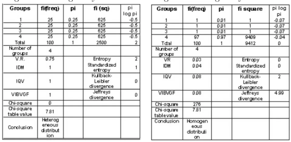
First, a qualitative distribution with 4 distinct categories is investigated (N=100). The most heterogeneous situation that is possible is imagined. For this kind of a frequency distribution, the summarizing qualitative variation statistics are as follows:

Table 1. Qualitative Variation Statistics for a distribution with 4 categories and with the highest degree of heterogeneity

Table 2. Qualitative Variation Statistics for a distribution with 4 categories and with the highest degree of homogeneity

Then a qualitative variation that can be the most homogeneous one with 4 categories is studied. The summarizing qualitative variation statistics are given below:

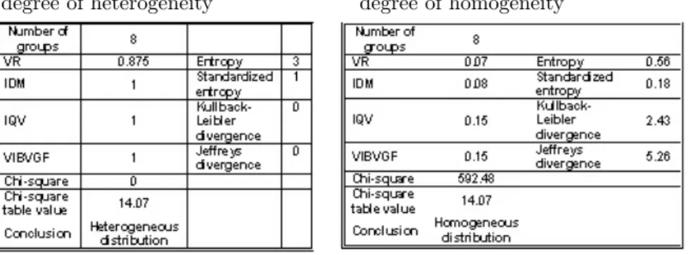
In addition , we have also investigated some qualitative distributions with 8 and 12 groups. For these applications , we have taken N=80, or N=120 to get integer numbers for the group frequencies. To make the picture clearer, we have simplified some of our findings in the following schemes. Table 3 (for the most heterogeneous distribution possible) and Table 4 (for the most homogeneous distribution possible) summarizes our findings for N=80 with 8 categories as below:

(9)

Table 5 (for the most heterogeneous distribution possible) and Table 6 (for the most homogeneous distribution possible) summarizes our findings for N=120 with 12 categories as below:

4. Conclusion

1) In this study, we have intended to show that some of the measures of qualitative variation are closely connected to each other. In this context, the variation index based on the variance of group frequencies (VIBVGF) and equiv-alently the index of qualitative variation (IQV) can be obtained by standardizing the following measures: i) Simpson’s diversity index , ii) The Coeﬃcient of Un-alikeability iii)Gini Concentration index. For this reason VIBVGF and IQV are two leading statistics among all. Similarly The Index of Deviations from The Mode (IDM) can be derived by standardizing The Variation Ratio (VR).

(10)

2) Although all these measures produced similar results one point should be highlighted: In the examples given above, we have observed that when the degree of heterogeneity is high, all these measures give similar results indepen-dently from the number of categories. But when the degree of homogeneity is high, these measures increase slightly due to the increase in the number of categories.

3) The variation index based on the variance of group frequencies (VIBVGF) and equivalently the index of qualitative variation (IQV) are closely related to a chi-square distribution under the null hypothesis that we have an extrmely het-erogeneous distribution. This result is especially important for further sampling distributions of these qualitative variation statistics.

4) The applications of measures based on entropy to qualitative variation sometimes result in some problems since there are some restrictions that origi-nated from logarithmic function involved in these definitions.

5) The asymptotic sampling properties of Kullback-Leibler divergence and Jeﬀreys divergence are studied in literature. So this may be a positive factor for choosing them among all these statistics. In this context, one can refer to Pardo(2006).

References

1. Cover, T.M.; Thomas, J.A.(2006): “Elements of Information Theory”, Wiley In-terscience (Second Edition), Hoboken, New Jersey

2. Cramér, H.(1999), “Mathematical Methods of Statistics”, Princeton Landmarks in Mathematics, Princeton University Press, USA, s206-207

3. Everitt,B.S.( 2006), “The Cambridge Dictionary of Statistics” , Cambridge Univer-sity Press (Third Edition), Cambridge

4. Jaynes, E.T.(2005),”Probability Theory The Logic of Science”,Cambridge Univer-sity Press, s345-351

5. Kader, G.D.&Perry, M. (2007), “Variability for Categorical Variables”, Journal of Statistics Education , Volume 15, Number 2 (2007), s2,

http://www.amstat.org/publications/jse/v15n2/kader.html

6. Kullback, S. (1997), “Information Theory and Statistics”, Dover Publications, New York, s6.

7. Garcia, A.L.(1994), “Probability and Random Processes for Electrical Engineering”, Addison-Wesley Longman (Second Edition)

8. Genceli, M.(1987) , “Statik Toplanma Ölçüleri”, ˙Istanbul Üniversitesi ˙Iktisat Fakül-tesi Mecmuası, C. 43, Prof. Dr. S.F. Ülgener’e Arma˘gan, ˙Istanbul

9. ˙Ipek, M. (1988), “˙Istatisti˘ge Giri¸s-I: Betimsel ˙Istatistik”, Beta Yayın Da˘gıtım A.¸S., ˙Istanbul

10. Pardo, L. (2006), “Statistical Inference Based on Divergence Measures”, Chap-man&Hall/CRC, USA, s64-92

11. Rényi, A.(2007) , “Probability Theory”, Dover Publications, New York, s540-603 12. Reza,Fazlollah M.(1994) , “An Introduction to Information Theory”, Dover Pub-lications, New York

(11)

13. Swanson, D.A.(1976), “A Sampling Distribution and Significance Test for Diﬀer-ences in Qualitative Variation”, Social Forces, Vol. 55, No.1, , University of North Carolina Press, s. 182-184

14. Upton, G.; Cook, I. (2006), “Oxford Dictionary of Statistics”, Oxford University Press (Second edition), NewYork

15. Weisberg, H.F.(1992), “Central Tendency and Variability”, Series: Quantitative Applications in the Social Sciences 83, Sage Publications, USA

16. Wilcox, A.R(1967) , “Indices of Qualitative Variation” , 1967, Oak Ridge National Laboratory; ORNL-TM-1919