Pamukkale Univ Muh Bilim Derg, 23(4), 451-461, 2017
Pamukkale Üniversitesi Mühendislik Bilimleri Dergisi
Pamukkale University Journal of Engineering Sciences
451
Optimal pricing policy with inventory related costs and reference effects
Stokla bağlantılı maliyetler ve referans etkisiyle en iyi fiyatlandırma
politikası
Mehmet Güray GÜLER1*, Mustafa AKAN2, İsmail SEVİM1
1Industrial Engineering Department, Machine Faculty, Yildiz Technical University, Istanbul, Turkey.
[email protected], [email protected]
2Department of Economics, School of Economics and Administrative Science, Dogus University, Istanbul, Turkey.
Received/Geliş Tarihi: 31.07.2016, Accepted/Kabul Tarihi: 24.11.2016
* Corresponding author/Yazışılan Yazar Research Article/doi: 10.5505/pajes.2017.49002 Araştırma Makalesi
Abstract Öz
This paper addresses the problem of a retailer who buys a certain amount of inventory at the start of a selling season. Holding inventory is costly and the demand is dependent on the current price and the reference price. The reference price is developed by customers and acts as a benchmark against the current price. The aim of the retailer is to maximize its discounted profit. The problem is modeled as an optimal control problem to determine the optimal pricing policy. For general demand models, the marginal cost due to an increase in the inventory and the marginal gain due to an increase in the reference price are provided analytically. For the linear demand models, the optimal pricing strategy is given explicitly and shown to be characterized by three stages: After a penetration or a skimming pricing strategy at the initial stage, the optimal price increases with time and the season ends with a discount. By introducing the reduced price which is the premium over the cost of the products, it is shown that the existence of procurement and holding cost is the driver for the increase in the price during the intermediary stage. The sensitivity of the optimal price to demand and cost parameters is also provided with a numerical study.
Bu çalışmada sezon başlamadan belirli miktarda ürün alan bir satıcının problemi ele alınmaktadır. Elde stok tutmanın bir maliyeti bulunmakla beraber talep mevcut fiyata ve referans fiyata bağlıdır. Referans fiyat müşteriler tarafından oluşturulmakta ve mevcut fiyatın miktarının ölçülmesi için kullanılmaktadır. Satıcının amacı kendi iskonto edilmiş karını eniyilemektir. Problem, en iyi fiyatlandırma politikasını bulmak üzere optimal kontrol problemi olarak modellenmiştir. Genel talep modelleri için, stok miktarındaki artışın sebep olduğu marjinal maliyet ve referans fiyatın artışının neden olduğu marjinal gelir miktarları analitik olarak sunulmuştur. Doğrusal talep modelleri için ise optimal fiyatlandırma stratejisi analitik olarak bulunmuş ve üç aşamalı olarak bulunan yapı açık bir şekilde sunulmuştur: İlk aşamadaki kaymağını alma veya nüfuz (penetrasyon) stratejisinden sonra optimal fiyat zamanla artmakta, ve satış sezonu bir indirim ile bitmektedir. Ürünün maliyetleri üzerine eklenen bir prim olarak tanımlanan indirgenmiş fiyatın tanımlanmasıyla, ikinci evredeki fiyat artışının ürünlerin satın alım ve elde tutma maliyetlerinden kaynaklandığı gösterilmiştir. Optimal fiyatın talep ve maliyet parametrelerine olan duyarlılığı ise sayısal çalışmalar ile gösterilmiştir.
Keywords: Pricing, Inventory, Reference price effects, Optimal
control Anahtar kelimeler: Fiyatlandırma, Stok, Referans fiyat etkisi, Optimal kontrol
1 Introduction
As customers buy a particular product frequently, they develop their own price expectations, which is called the reference price. The reference price is an inherent benchmark used for the actual prices and the consumers make decisions by comparing the actual prices with the reference price [1]. Consider a retailer in apparel sector. The demand of the clothes is seasonal in the sense that the demand is effective only in a “season” like winter or summer. The retailer faces a downward sloping demand curve, orders a certain amount of the good at the beginning of the season and aims to maximize its profit for the season by selling the products. The retailer can change the demand during the selling season by changing the price of the product. However, the demand is not dependent only on the price. The customers treat the reference price as a standard for the actual price and the demand is influenced by the reference price as well. If the actual price is less than the reference price, the demand is positively influenced by this variation. However, the reference price evolves through time and a permanent discount reduces the reference price which makes the customers think that the
product is worth less. Therefore, although reducing the price increases the current demand, it has a negative effect on the future profits through the reference price which is called the reference effect. In this study, we analyze a retailer which sells a single product whose demand is under reference effects. A retailer that sells fashion goods that are exported from China or similar countries is an example. Such a retailer has a single opportunity to give an order and receives all of the products at the beginning of the selling season. Since the goods are fashion products, they must be sold in that particular season and almost have no value for the next year. Hence the retailer has to decide on the quantity to be ordered and the price of the product. Since the demand is affected by the reference price, the retailer has to think twice when making a discount since it will lower the demand in following weeks. Our aim is to find the optimal pricing policy of the retailer in a continuous time setting when the planning horizon is finite.
In their seminal work, [2] studied the periodic review multi-period problem without a setup cost where the unmet orders are backordered. They discussed the optimality of a base-stock list-price policy where a linear demand function is observed. This policy indicates that an optimum inventory-price pair can
Pamukkale Univ Muh Bilim Derg, 23(4), 451-461, 2017 M. G. Güler, M. Akan, İ. Sevim
452 be found at each period and if on-hand inventory is below the
optimal inventory level, then the seller places an order to raise the on-hand inventory to that level and sets the optimum price. Otherwise, it doesn’t place any order and picks a selling price which is less than the optimum price. [3],[4] introduced a setup cost to the setting of [2]. [5] analyzed a system where there exists a pile of levers to control the demand which is assumed to be concave over these levers. In the studies mentioned, the optimal policy seems to be a version of a (𝑠, 𝑆, 𝑝) policy. This policy indicates that if on hand inventory is below 𝑠, then the seller makes an order to bring its inventory level to 𝑆 such that 𝑠 ≤ 𝑆 and declares the price 𝑝. On the contrary it orders nothing and declares a state dependent price. The studies above does not consider the reference price effects. In this study, we deal with reference price effects as well. [6],[7] provided a literature review on joint pricing and replenishment/inventory decisions.
The theoretical basis of reference price comes from adaptation level theory [8]. The theory indicates that expectation-based reference price is the adaptation level against which actual prices are judged [9]. A major issue is to understand the systematic behavior of consumers on forming expectations (i.e. how reference prices change) in time. Exponential smoothing model arising from the adaptive expectation model is a widely preferred form for the change of the reference price [10] but is not the only one [11]. [12],[13] give a literature review of models taking account of reference prices. We employ the widely used exponential smoothing model in our setting.
[14] studied dynamic pricing under deterministic linear demand with reference effects in a continuous time framework. In the study, the steady state prices are calculated and it is concluded that a seller should decide on using a penetration or a skimming strategy which depends on the initial reference price. [15] studied the same problem when time is discrete for more general demand models. They showed that the optimality of the penetration or the skimming strategies is also true for non-linear demand models as well. These studies did not incorporate the inventory decision whereas we explicitly model the inventory in our setting. In the joint inventory and pricing literature, the researchers employ an additive and/or a multiplicative random term to model the randomness in the demand functions. [16]-[19] studied joint inventory and pricing problem with stochastic linear demand under reference effects with discrete time setting. [16] simulated the multi-period problem in case of linearity of the demand where the randomness is caused by an additional random term and showed that state-dependent order-up-to is optimal in the simulation. [19] studied problems with two periods and showed the optimality of a state-dependent order-up-to policy for two periods. In the state-dependent order-up-to policy, the order-up-to level depends on the state, particularly on the reference price. [17],[18] showed the optimality of a state-dependent order-up-to policy for the stochastic linear demand models with finite or infinite time horizon. [18] additionally showed the convergence of reference price, i.e., they show that the system converges to a steady state and characterized it. Moreover they showed that the optimal order-up-to level was shown to increase with the reference price. [20],[21] studied concave demand models and showed the optimality of the state-dependent order-up-to policy. [21] showed that two subproblems can be obtained by decomposing the problem
and the optimal pricing and inventory policy are characterized by using these subproblems. They also provided the solutions for the optimal parameters. The researchers in [16]-[21] address similar problems under a discrete time and periodic review setting. In this setting the retailer can make a replenishment at every period whereas in our setting the retailer can place an order only at the beginning of the horizon. Moreover they study a stochastic setting and we study a deterministic setting which allows use to use optimal control theory. The optimal control theory provides the optimal function, instead of optimal values, i.e., one can find the explicit function of the decision variables.
Recently, [22] dealt with very similar problem where the inventory decays throughout time when the demand is linear. In this study, we also provide analysis on general demand models. Moreover we analyze the linear demand models in a more detailed way in our numerical illustrations.
Analytical solutions for problems with reference effects have a stochastic nature and multi-periodicity property are analyzed in above studies. For a single period model readers are referred to [23] where the author showed that reference price affects the profitability of a company significantly.
The literature on the analysis under reference effects has been developing fast in the last years. The analysis focused on several extensions like stochastic reference prices [24]-[26], supply chain and coordination [27],[28], advertising [29],[30] and technology investment [31].
The joint inventory and pricing decisions with reference effects are studied in the context of stochastic demand models. The analytical results in this line of research are limited due to the stochastic nature. The deterministic models, on the other hand, do not incorporate inventory decisions. We extend the deterministic line of the literature by incorporating inventory holding cost. We provide the marginal effect of a unit inventory and a unit reference price on the total profitability for the general demand models analytically. To the best of our knowledge, this is the first study providing the analytical solutions for such marginal effects on a demand model with reference effect. For the linear demand models, we provided explicit closed form solutions for the optimal pricing policy. [14] provided explicit closed form solutions as well, however our model is an extension of their model by introducing inventory as the state and incorporating the inventory holding cost. Finally, we resort to numerical studies for sensitivity analysis of the price.
We observe that the optimal pricing strategy can be characterized by three stages. The pricing strategy of the initial stage depends on the initial reference price. There exists a skimming strategy if the initial reference price is high. Otherwise, a penetration strategy is optimal. After the initial stage, the optimal price increases until the discount at the end of the season.
The next section describes a demand model with reference effects and gives a parametric solution of optimal control model for the pricing problem. Sensitivity analysis of the optimal price to the demand, cost, and reference effect parameters is provided in Section 3. Finally the conclusions are given in Section 4. An Appendix is provided for derivation of the results.
Pamukkale Univ Muh Bilim Derg, 23(4), 451-461, 2017 M. G. Güler, M. Akan, İ. Sevim
453
2 The model
In this section, we give our setting, assumptions and formulate the problem as an optimal control problem. We consider a retailer of a seasonal product. At the beginning of each season, the retailer orders and receives the products before the selling season. There is no another replenishment opportunity, hence the retailer has to decide taking into account the entire selling season. We focus on a single product whose demand is dependent on the current price and the reference price. The customers compare the current price with the reference price and the demand is affected by the difference between two prices. The consumers develop the shared reference price using the past data of the prices of the product and update their reference price levels with the introduction of new price levels. The evolution of the reference price can be modelled by appropriate models. The exponential smoothing model is widely used for such purpose [12]. Therefore, the reference price formation is given by the following ordinary differential equation [14]:
𝑟′= 𝛽(𝑝(𝑡) − 𝑟(𝑡)) (1)
Where 𝑝 denotes the price, 𝑟 denotes the reference price, 𝑡 denotes the time, 𝑓′= 𝑑𝑓/𝑑𝑡 for any function 𝑓, 𝛽 is the
memory parameter and 0 ≤ 𝛽 ≤ 1. When 𝛽, the memory parameter, is low the reference price are affected mostly by the price history. When 𝛽, the memory parameter, is high the reference price are affected mostly by the current price. The retailer incurs a procurement cost of 𝑐 per product at the beginning of the season, collects the sales revenue, and incurs a holding cost at a rate of ℎ per unit product. The objective of the retailer is to maximize its profit by choosing its pricing strategy optimally. We formulate the problem using optimal control. The total profit is given by the following:
𝑚𝑎𝑥 𝑝(𝑡)≥0∫ 𝑒 −𝑖𝑡(𝑝(𝑡)𝑄(𝑝(𝑡), 𝑟(𝑡), 𝑡) − ℎ𝐼(𝑡))𝑑𝑡 𝑇 𝑜 − 𝑐𝐼0 (2) 𝐼′(𝑡) = −𝑄(𝑝(𝑡), 𝑟(𝑡), 𝑡) (3)
where 𝑇 denotes the length of the season, 𝐼(𝑡) denotes the inventory level at time 𝑡 and 𝑄(𝑡) denotes the demand curve. The initial reference price is a parameter and is given as 𝑟(0) = 𝑟0. It is assumed that all the products have to be sold
during the selling season and no products are left at the end of the horizon, i.e., 𝐼(𝑇) = 0. This is intuitive since there is no salvage value at the end of the selling season. The initial inventory level 𝐼(0) is to be chosen optimally by the retailer since once the optimal pricing policy is explicitly characterized by the solution, one can calculate the inventory level at any instance. Hence there is no boundary condition on the initial inventory level (𝜆1(𝑇) = 0). First we analyze a general form of
demand. Then we employ a linear demand model to come up with an explicit solution.
2.1 A general demand model
The Current Value Hamiltonian of the problem is given by: 𝐻 = 𝑝𝑄 − ℎ𝐼 − 𝜆1𝑄 + 𝜆2𝛽(𝑝 − 𝑟).
Together with the equation (1), the necessary conditions for the optimal solution are:
𝐻𝑝= 0 (4) 𝜆1′ = 𝜆1𝑖 − 𝜕𝐻 𝜕𝐼 (5) 𝜆2′ = 𝜆2𝑖 − 𝜕𝐻 𝜕𝑟 (6) 𝐼′(𝑡) = −𝑄(𝑝(𝑡), 𝑟(𝑡), 𝑡) (7)
The equation (4) can be written as: 𝜕(𝑝𝑄)
𝜕𝑝 + 𝜆2𝛽 = 𝜆1𝑄𝑝 (8)
Where 𝑄𝑝 denotes the partial derivative of the demand with
respect to the price. Recall that the 𝜆 variables are the current value multipliers: 𝜆1 shows the current cost of having one
more unit of inventory and 𝜆2 shows the current cost of
starting with one more unit of reference price. The term (𝜕(𝑝𝑄)𝜕𝑝 ) shows the marginal increase in the revenue due to a unit increase in 𝑝. Next, consider the term 𝜆2𝛽. A unit increase
in 𝑝 results in an increase of 𝛽 units in 𝑟 since the reference price is updated with Equation (1). Therefore, 𝜆2𝛽 shows the
increase in the profit due to the increase in the price through the reference price effect. Finally, consider the term 𝜆1𝑄𝑝. 𝑄𝑝
shows the marginal decrease in the demand with a unit increase in 𝑝, hence it is the inventory left due to the price increase. 𝜆1𝑄𝑝, therefore, shows the marginal decrease in the
profit due to the increase in the price through the inventory. As a result, the left hand side of Equation (8) is the marginal income received by increasing the price (on current profit and future profit) and the right hand side represents marginal cost incurred by increasing the price. Therefore Equation (8) shows the classical optimality condition: the marginal cost should be equal to the marginal income.
The necessary condition for 𝜆1 in Equation (9) is given by
𝜆1′ = 𝜆1𝑖 + ℎ which gives 𝜆1= 𝑒𝑖𝑡−ℎ𝑖. Here 𝑀1 is a constant to
be found from the terminal condition 𝜆1(0) = 𝑐 and is given by
𝑀1=ℎ+𝑖𝑐𝑖 . The value of 𝜆1, therefore, can be written as follows:
𝜆1=
ℎ
𝑖(𝑒𝑖𝑡− 1) + (𝑒𝑖𝑡𝑐) (9)
The present value of paying the holding cost ℎ continuously for a duration of 𝑡 time units is given by ∫ ℎ𝑒𝑡 −𝑖𝑡
0 which is equal
to ℎ𝑖(1 − 𝑒𝑖𝑡). In other words, ℎ
𝑖(1 − 𝑒𝑖𝑡) is the present value
of cost of holding an item which is sold at time 𝑡. The current value of the holding cost is ℎ𝑖(𝑒𝑖𝑡− 1) which is the first term in
Equation (9). For the other term, note that every item is purchased at the beginning of the planning horizon, hence the present value of procurement cost is 𝑐 for every item. The current value of the procurement cost that is sold at time 𝑡 is, therefore, given by 𝑐𝑒𝑖𝑡 which is the second term in Equation
(9). As a result, 𝜆1 is the current cost of having one more unit
of inventory which is the current value of the sum of procurement cost and the inventory cost.
Rewriting the necessary Equation (8), we get:
𝜆2′ = 𝜆2(𝑖 + 𝛽) + (𝜆1− 𝑝)𝑄𝑟, (10)
Where 𝑄𝑟 denotes the partial derivative of the demand with
Pamukkale Univ Muh Bilim Derg, 23(4), 451-461, 2017 M. G. Güler, M. Akan, İ. Sevim
454 marginal increase of the reference price at time 𝑡 on the
profitability and it is given by the following:
𝜆2(𝑡) = ∫ 𝑒𝑡𝑇 −(𝑖+𝛽)(𝑠−𝑡)𝑄𝑟(𝑠)(𝑝(𝑠) − 𝜆1(𝑠))𝑑𝑠 (11)
Recall that 𝜆1 denotes the current value of the cost of an item
(the holding and the procurement cost). The term 𝑝(𝑠) − 𝜆1(𝑠)
is, therefore, the profit per unit at time 𝑠. The term 𝑄𝑟(𝑠)
denotes the marginal increase in the demand with a unit increase in the reference price. The exponential term 𝑒−(𝑖+𝛽)(𝑠−𝑡) represents discounting which includes the interest
rate 𝑖 and the memory parameter 𝛽 that shows the forgetting rate of the reference price by the customers. The integral, therefore, represents the present value (at time 𝑡) of the profit of the company due to marginal increase in the reference price. The necessary conditions in Equation (1) and Equations (6)-(7) can be reduced into a non-linear first order system of equations. However, an exact solution cannot be found without an explicitly known function of 𝑄(𝑝(𝑡), 𝑟(𝑡), 𝑡). Hence, in the next section we analyze the problem with a linear demand function.
2.2 A linear demand model
In this section we analyze a linear demand model. The demand curve is given by the following equation:
𝑄(𝑡) = 𝑚 − 𝑛𝑝(𝑡) − 𝛾(𝑝(𝑡) − 𝑟(𝑡)) (12)
where 𝑚 and 𝑛 are the non-negative parameters of the download sloping demand curve. 𝛾 is the reference effect impact and 𝛾 > 0. The time is denoted by 𝑡. The current price and the reference price at time 𝑡 are denoted by 𝑝(𝑡) and 𝑟(𝑡), respectively. The model in Equation (9) was employed in [14],[17],[18],[32],[33].
The necessary condition in Equation (8) can be written as: 𝐻𝑝= (𝑚 − 2𝑛𝑝 − 𝛾(2𝑝 − 𝑟)) + 𝜆1(𝑛 + 𝛾) + 𝜆2𝛽 =
0 (13)
Solving 𝑝 from Equation (10) yields: 𝑝 =𝑚+𝛾𝑟+𝜆2𝛽
2(𝛾+𝑛) +
𝜆1
2 (14)
Substituting Equation (14) into Equations (1) and (8) yields: 𝑟′= 𝛽 [𝑚+𝛾𝑟 2(𝛾+𝑛)+ 𝜆1 2+ 𝜆2𝛽 2(𝛾+𝑛)− 𝑟] (15) 𝜆2′ = 𝜆2[𝑖 −2(𝛾+𝑛)𝛾𝛽 + 𝛽] −2(𝛾+𝑛)𝑚𝛾 − 𝛾 2 2(𝛾+𝑛)𝑟 + 𝛾𝜆1 2 (16)
Now we substitute 𝜆1 from Equation (9) and rearrange terms
in Equations (15)-(16): 𝑟′= 𝛽 [ 𝑚 2(𝛾+𝑛)− ℎ 2𝑖+ 1 2 ℎ+𝑖𝑐 𝑖 𝑒 𝑖𝑡−(𝛾+2𝑛) 2(𝛾+𝑛)𝑟 + 𝛽 2(𝛾+𝑛)𝜆2] (17) 𝜆2′ = −2(𝛾+𝑛)𝑚𝛾 −ℎ𝛾2𝑖+𝛾2ℎ+𝑖𝑐𝑖 𝑒𝑖𝑡+ [𝑖 −2(𝛾+𝑛)𝛾𝛽 + 𝛽] 𝜆2− 𝛾 2 2(𝛾+𝑛)𝑟 (18) After some tedious algebra, the solution for this system of differential equations is given as:
𝜆2(𝑡) =𝑖(𝐾𝑎+𝐾̂0)𝑒 𝐾0+𝑖 2 𝑡𝐶2+𝑖(𝐾𝑎+𝐾̂0)𝑒− 𝐾0−𝑖 2 𝑡𝐶1−𝐾𝑐𝑒𝑖𝑡+𝐾𝑑 𝑖𝛽2 (19) 𝑟(𝑡) = 𝑒𝐾02 𝑡+𝑖𝐶2+ 𝑒−𝐾02 𝑡−𝑖 𝐶1+ 𝐾𝑒𝑒𝑖𝑡+ 𝐾𝑏, (20)
where the constants are given in Appendix A. Substituting the values of 𝑟 and 𝜆2 into the price equation in Equation (14) and
after some algebra, the price is given as: 𝑝(𝑡) = 𝐾+𝑒
𝐾0+𝑖
2 𝑡𝐶2+ 𝐾−𝑒−𝐾02 𝑡−𝑖𝐶1+ 𝐾𝑖𝑒𝑖𝑡+ 𝐾𝑏 (21)
where the constants 𝐾+≥ 0, 𝐾−≥ 0, 𝐾𝑖≥ 0 and 𝐾𝑏 are given
in Appendix B. Appendix C shows that the Equations (19)-(21) satisfy the necessary condition in Equation (8).
The inventory can be found by solving the state equation 𝐼′(𝑡) = −𝑄(𝑡) and is given by the following:
I(t) = (𝑛𝐾𝑏− 𝑚)𝑡 + (𝑖+𝐾2𝑛 0+ 𝑛+𝛾 𝛽 ) 𝑒 𝑒𝐾0+𝑖2 𝑡𝐶2+ (𝑖−𝐾2𝑛 0+ 𝑛+𝛾 𝛽 ) 𝑒 −𝐾0−𝑖2 𝑡𝐶 1+ (𝑖𝑛𝐾2𝛾𝛽𝑐) 𝑒𝑖𝑡+ 𝐶𝑄. (22) Here 𝐶𝑄 is the coefficient of integration to be found from the
boundary condition 𝐼(𝑡) = 0 and is given as: 𝐶𝑄= (𝑚 − 𝑛𝐾𝑏)𝑇 − (𝑖+𝐾2𝑛 0+ 𝑛+𝛾 𝛽 ) 𝑒 𝑒𝐾0+𝑖2 𝑡𝐶2− (𝑖−𝐾2𝑛 0+ 𝑛+𝛾 𝛽 ) 𝑒 −𝐾0−𝑖2 𝑡𝐶 1− (𝑖𝑛𝐾2𝛾𝛽𝑐) 𝑒𝑖𝑡. (23) Although the closed form solution for the optimal price is given in Equation (21), it is difficult to make a sensitivity analysis over the parameters. Therefore, we resort to numerical illustrations to understand the effects of the parameters on optimal pricing policy.
3 Sensitivity analysis of optimal price
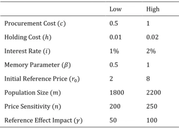
In this section, the sensitivity analysis of optimal price to the cost and demand parameters is provided. The optimal price path is plotted at low and high values for the parameters which are given in Table 1. At every plot, unless it is stated otherwise, all of the parameters (except the parameter under study) are set to their high values. That is, we set the parameters to their high values, and change the value of the parameter under study to see the sensitivity of the price to that parameter. The plots where all of the parameters are set to their low values (except the parameter under study) are given in Appendix D.Table 1: Parameter values.
Low High
Procurement Cost (𝑐) 0.5 1
Holding Cost (ℎ) 0.01 0.02
Interest Rate (𝑖) 1% 2%
Memory Parameter (𝛽) 0.5 1
Initial Reference Price (𝑟0) 2 8
Population Size (𝑚) 1800 2200
Price Sensitivity (𝑛) 200 250
Pamukkale Univ Muh Bilim Derg, 23(4), 451-461, 2017 M. G. Güler, M. Akan, İ. Sevim
455 We substitute the values of the parameters in Table 1 into
Equation (21) and write the optimal price path explicitly to illustrate the values of the coefficients. In particular, the low values are substituted to find the optimal price path in Equation (24) and the high values are substituted to find the optimal price path in Equation (25).
𝑝(𝑡) = 1.9145𝑒0.4572𝑡+ 0.1055𝑒−0.4472𝑡+
0.7842𝑒0.01𝑡+ 3.9878 (24)
𝑝(𝑡) = 1.8653𝑒0.8653𝑡+ 0.1547𝑒−0.8453𝑡+
0.9961𝑒0.02𝑡+ 3.8809 (25)
3.1 Reference effect parameters
In this section, the sensitivity of the optimal price to the initial reference price 𝑟0 and the memory parameter 𝛽 are analyzed.
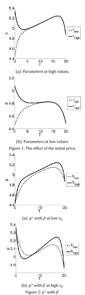
Figure 1(a) shows the optimal price path when all parameters but 𝑟0 are set to their high values. The solid line shows 𝑝(𝑡)
when 𝑟0 is high and the dashed line shows 𝑝(𝑡) when 𝑟0 is low,
as it can be observed from the legend on the right of the plot. Similarly, Figure 1(b) shows the optimal price path when all parameters but 𝑟0 are set to their low values. The solid line
and the dashed line show high and low values of 𝑟0,
respectively.
The following can be observed from Figure 1. The retailer starts with a low price and increases it gradually if 𝑟0 is low (a
penetration strategy). By the end of the season, the retailer decreases the price to sell off the inventory. If the initial reference price is high, the retailer behaves similarly after skimming strategy at the initial stage. Therefore, the optimal strategy and the level of optimal price are the same for both 𝑟0
levels after the initial stage. In fact, this three-fold pricing strategy will be shown to be optimal in all cases: After an initial penetration or a skimming strategy depending on the initial reference price, the price increases until the end of the season and there is a discount at the end to sell of the inventory. This policy is similar to the zero holding cost case in [14], except the price increase after the initial stage. [14] showed that after a penetration or a skimming strategy, the price resides at a constant price, which was shown to be the steady state price of the infinite horizon problem. The steady state price value is shown to be independent of the initial reference price. At the final stage, there is a discount since there is no need for long-term reference effect considerations. The optimal price in our setting (when there is a positive holding cost) increases until the discount at the end of the horizon instead of staying constant at the steady state price. The initial reference price has a substantial effect on the price path. Therefore, from this point on, the optimal price paths for each parameter will be plotted at both low and high 𝑟0 levels.
In particular, two plots are presented for each parameter. The plots on the left and right show the optimal price path when 𝑟0
is low and high, respectively. In both plots, the dashed line shows the optimal price when the particular parameter is at its low value and the solid line shows the optimal price when the particular parameter is at its high value.
Figure 2shows the sensitivity of the optimal price path to the memory parameter. [15] showed that the optimal price attains the steady state faster and starts the discount later if 𝛽 is low because of the exponential smoothing effect in Equation (1). The same observation can be made in Figure 2. The optimal price gets into the increasing trend faster and goes to a discount later when 𝛽 is high.
(a): Parameters at high values.
(b): Parameters at low values. Figure 1: The effect of the initial price.
(a): 𝑝∗ with 𝛽 at low 𝑟 0.
(b): 𝑝∗ with 𝛽 at high 𝑟 0.
Figure 2: 𝑝∗ with 𝛽.
3.2 Cost parameters (𝒄, 𝒉, and 𝒊)
In this section, we analyze the sensitivity of the optimal price to the procurement cost 𝑐, holding cost ℎ and the interest rate
Pamukkale Univ Muh Bilim Derg, 23(4), 451-461, 2017 M. G. Güler, M. Akan, İ. Sevim
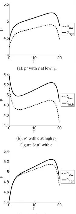
456 𝑖. Figure 3 shows the sensitivity of the optimal price path to
the procurement cost 𝑐. The retailer charges high prices when the procurement cost is high which is intuitive since the retailer should sell the costly products at higher prices. Figure 4 shows the sensitivity of the optimal price path to the holding cost ℎ. Since holding inventory is costly, the retailer charges higher price to make profit, as in the case of the procurement cost.
Figure 5 shows the sensitivity of the optimal price path to the interest rate 𝑖. The pricing behavior in this case is also similar to the cases of 𝑐 and ℎ, i.e., the retailer charges higher prices when the parameter is high. This is due to the fact that the interest rate is a cost item as ℎ or 𝑐: it is the opportunity cost of money tied up in inventories. Note that the optimal policy is the same for 𝑐, ℎ and 𝑖: after an initial penetration or a skimming strategy, the price increases until the end of the horizon and the season ends with a discount.
(a): 𝑝∗ with 𝑐 at low 𝑟 0.
(b): 𝑝∗ with 𝑐 at high 𝑟 0.
Figure 3: 𝑝∗ with 𝑐.
(a): 𝑝∗ with ℎ at low 𝑟 0.
(b): 𝑝∗ with ℎ at high 𝑟 0.
Figure 4: 𝑝∗ with ℎ.
(a): 𝑝∗ with 𝑖 at low 𝑟 0.
(b): 𝑝∗ with 𝑖 at high 𝑟 0.
Figure 5: 𝑝∗ with 𝑖.
3.3 Demand parameters (𝒎, 𝒏, 𝜸)
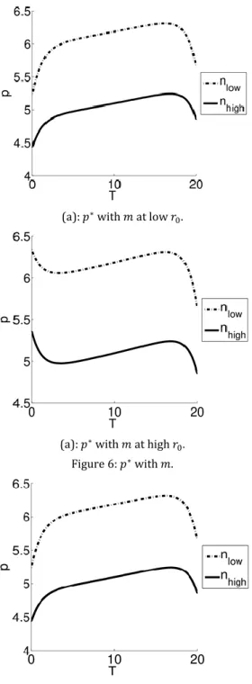
In this section, the sensitivity of the optimal price to the demand parameters is studied. Figure 6 shows the sensitivity of the optimal price path to the population size 𝑚 which is the maximum amount of demand that can be achieved when the price is zero. The number of customers, who buy the product at a certain level, increases as 𝑚 increases. The retailer, therefore, charges higher prices as 𝑚 increases.
Figure 7 shows the sensitivity of the optimal price path to the price sensitivity of the demand 𝑛. The price sensitivity 𝑛 is an indication for the monopolistic structure of the market. If 𝑛 is low, then the retailer (or market) is close to a monopoly. Therefore, the retailer facing a steep demand curve will set higher prices as observed in Figure 7. Figure 8 shows the sensitivity of the optimal price path to the reference effect impact 𝛾. It can be observed that the initial pricing strategy is less steep when 𝛾 is low. After the initial pricing period, the optimal price is always lower when 𝛾 is high.
Pamukkale Univ Muh Bilim Derg, 23(4), 451-461, 2017 M. G. Güler, M. Akan, İ. Sevim
457
3.4 The pricing strategy
The optimal pricing policy, in all of the cases above, is to start with a penetration or a skimming strategy and increase the price until the discount at the end of the horizon. There are two factors that contribute to the increasing trend of the optimal price during the intermediary stage. First, [14],[15] use 𝑐 as the procurement cost per unit which is charged at the
time of selling the product. In our model, 𝑐 is the procurement
cost and all units are purchased at the beginning of the period at a unit cost of 𝑐. The current value of the procurement cost of a product that is sold at time 𝑡 is given by 𝒄𝒆𝒊𝒕. Therefore the
current value of the procurement cost increases with time (if 𝑖 > 0). In order to compensate this, the retailer increases the price with time.
(a): 𝑝∗ with 𝑚 at low 𝑟 0.
(a): 𝑝∗ with 𝑚 at high 𝑟 0.
Figure 6: 𝑝∗ with 𝑚.
(a): 𝑝∗ with 𝑛 at low 𝑟 0.
b): 𝑝∗ with 𝑛 at high 𝑟 0.
Figure 7: 𝑝∗ with 𝑛.
(a): p^* with γ at low r_0.
(b) p^* with γ at high r_0. Figure 8: p^* with γ.
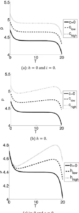
Figure 8(a) shows the optimal price path with procurement cost 𝑐 when the interest rate and inventory holding cost are zero (𝑖 = 0, ℎ = 0). The optimal price attains a constant value after the initial stage as in the case of [14], [15]. This is due to the fact that the current value of the procurement cost stays constant since 𝑖 = 0. This behaviour changes if there is a positive interest rate. Figure 8(b) shows the optimal price path at different levels of 𝑐 when there is low interest rate and zero inventory holding cost (𝑖 = 𝑖𝑙𝑜𝑤, ℎ = 0). Second, the
current value of the holding cost of an item sold at time 𝑡 is
𝒉 𝒊(𝒆
𝒊𝒕− 𝟏) which increases with time. Hence the holding cost
has the same effect with the procurement cost. Figure 8(c) shows the optimal price path with respect to the holding cost
Pamukkale Univ Muh Bilim Derg, 23(4), 451-461, 2017 M. G. Güler, M. Akan, İ. Sevim
458 when the interest rate and procurement cost are zero
(𝑖 = 0, 𝑐 = 0). Therefore, both the holding cost and the procurement cost contribute to the increasing trend of the optimal pricing strategy. It can be concluded that the cost of having one unit of inventory, which is given by 𝜆1 and found to
be the current value of the sum of procurement cost and the inventory cost, is the reason behind the price increase during the intermediary stage. This can also be justified by plotting the reduced price which is obtained by eliminating the effect of 𝜆1 from the optimal price path given in Equation (14). Let
𝑝𝑟(𝑡) = 𝑝(𝑡) − 𝜆
1(𝑡)/2 denote the reduced price. The reduced
price is a kind of premium over the product costs, i.e., the procurement cost and the inventory holding cost. Figure 9(a) and Figure 9(b) show the value of the reduced price when all parameters are at low and high values, respectively. It can be observed that there is still a penetration or a skimming strategy based on the initial reference price.
(a): ℎ = 0 and 𝑖 = 0.
(b) ℎ = 0.
(c) i= 0 and 𝑐 = 0.
Figure 8: Effect of costs on pricing strategy.
(a): 𝑝𝑟(𝑡) with low parameter values.
(b): 𝑝𝑟(𝑡) with high parameter values.
Figure 9: 𝑝∗ with 𝛾.
The retailer starts with a high or a low value at the initial stage, depending on the initial reference price. Then the retailer fixes the value of 𝑝𝑟(𝑡) just like the case in [14] after
the initial stage and then reduces it at the end of the horizon. This shows that our results in fact confirm the previous results in [14]. Please note that the time horizon is set to 40 in order to see the effect of constant profit margin better.
4 Conclusions
We study the problem of a retailer who buys a certain amount of inventory at the start of a selling season. Holding inventory is costly and there is a reference effect on the demand. The aim of the retailer is to maximize its discounted profit through a finite horizon.
For general demand models, we provide analytical solutions for marginal effects of the inventory and the reference price. The marginal effect of an inventory is the sum of the present value of the procurement cost and total holding cost incurred. The marginal effect of the reference price is the discounted sum of the profit rate weighted with the marginal increase in the demand due to a unit increase in the reference price. For the linear demand model, we provide explicit solution of the optimal price. The optimal pricing strategy can be characterized by three stages. The initial stage is a penetration or a skimming strategy depending on the initial reference price. After the initial stage, the optimal price increases due to the procurement cost and the holding cost. Although this result does not seem to be confirmed by the previous results, we justify it by introducing the reduced price which can be defined as the premium over the cost of the product. It is shown that the reduced price just follows the same path with
Pamukkale Univ Muh Bilim Derg, 23(4), 451-461, 2017 M. G. Güler, M. Akan, İ. Sevim
459 the previous results in the literature, i.e., it stays constant after
the initial stage. In the final stage there is a deep discount, which is observed in reality, since towards the end of the planning interval there is no need to make long-term reference price considerations. The initial reference price is the most important factor effecting the price strategy as observed in all cases. All parameters, except the initial reference price, effect the price level but not the strategy. We also provide sensitivity analysis of the optimal price to the cost and demand parameters. We show that the retailer charges a higher price as the cost parameters increase as expected.
The researchers provide several analytical results in the operations research literature, however there are very few studies showing the real effect of reference price on the inventory and pricing decisions with the real data. Such an attempt would be valuable future work. Another research venue is to investigate whether the results of this study can be generalized to other demand models.
5 References
[1] Kalyanaram G, Winer RS. “Empirical generalizations from reference price research”. Marketing Science, 14(3), 161-169, 1995.
[2] Federgruen A, Heching A. “Combined pricing and inventory control under uncertainty”. Operations
Research, 47(3), 454-475, 1999.
[3] Chen X, Simchi-Levi D. “Coordinating inventory control and pricing strategies with random demand and fixed ordering cost: The finite horizon case”. Operations
Research, 52(6), 887-896, 2004.
[4] Chen X, Simchi-Levi D. “Coordinating inventory control and pricing strategies with random demand and fixed ordering cost: The finite horizon case”. Mathematics of
Operations Research, 29(3), 698-723, 2004.
[5] Huh WT, Janakiraman G, “(s,S) optimality in joint inventory-pricing control: An alternate approach”,
Operations Research, 56(3), 783-790, 2008.
[6] Elmaghraby W, Keskinocak P. “Dynamic pricing in the presence of inventory considerations: Research overview, current practices, and future directions”.
Management Science, 49(10), 1287-1309, 2003.
[7] Chen X, Simchi-Levi D. Pricing and Inventory
Management. Handbook of Pricing Management, Oxford,
United Kingdom, Oxford University Press, 2012.
[8] Helson M. Adaptation Level Theory. New York, USA, Harper and Row, 1964.
[9] Monroe KB. “Buyers' subjective perceptions of price”.
Journal of Marketing Research, 10, 70-80, 1973.
[10] Nerlove M. “Adaptive expectations and cobweb phenomena”. Quarterly Journal of Economics, 72, 227-240, 1958.
[11] Nasiry J, Popescu I. “Dynamic pricing with loss-averse consumers and peak-end anchoring”. Operations
Research, 59(6), 1361-1368, 2011.
[12] Mazumdar T, Raj SP, Sinha I. “Reference price research: Review and propositions”. Journal of Marketing, 69(4), 84-102, 2005.
[13] Arslan H, Kachani S. Dynamic Pricing Under Consumer
Reference‐Price Effects. Editors: Cochran JJ, Cox LA,
Keskinocak P, Kharoufeh JP, Smith JC. Wiley Encyclopedia of Operations Research and Management Science, 1-8, Hoboken, NJ, USA, Wiley, 2011.
[14] Fibich G, Gavious A, Lowengart O. “Explicit solutions of optimization models and differential games with nonsmooth (asymmetric) reference-price effects”.
Operations Research, 51(5), 721-734, 2003.
[15] Popescu I, Wu Y. “Dynamic pricing strategies with reference effects”. Operations Research, 55(3), 413-429, 2007.
[16] Gimple-Heersink L, Rudloff C, Fleischmann M, Taudes A. “Integrating pricing and inventory control: is it worth the effort?”. BuR Business Research Journal, 1(1), 106-123, 2008.
[17] Zhang Y. Essays on Robust Optimization, Integrated Inventory and Pricing, and Reference Price Effect. PhD Thesis, University of Illinois at Urbana-Champaign, Illinois, USA, 2010.
[18] Chen X, Hu P, Shum S, Zhang Y. “Stochastic inventory models with reference price effects”. Working Paper. [19] Taudes A, Rudloff C. “Integrating inventory control and a
price change in the presence of reference price effects: A two-period model”. Mathematical Methods of Operations
Research, 75(1), 1-37, 2012.
[20] Guler MG, Bilgic T, Gullu R. “Joint inventory and pricing decisions with reference effects”. IEE Transactions, 46(4), 330-343, 2014.
[21] Guler MG, Bilgic T, Gullu R. “Joint pricing and inventory control for additive demand models with reference effects”. Annals of Operations Research, 226(1), 255-276, 2015.
[22] Xue M, Tang W, Zhang J. “Optimal dynamic pricing for deteriorating items with reference-price effects”.
International Journal of Systems Science, 47(9), 1-10,
2014.
[23] Urban TL. “Coordinating pricing and inventory decisions under reference price effects”. International Journal of
Manufacturing Technology and Management, 13(1),
78-94, 2008.
[24] Baron O, Hu M, Najafi-Asadolahi S, Qian Q. “Newsvendor selling to loss-averse consumers with stochastic reference points”. Manufacturing & Service Operations
Management, 17(4), 456-469, 2015.
[25] Bi W, Li G, Liu M. “Dynamic pricing with stochastic reference effects based on a finite memory window”.
International Journal of Production Research, 55(12),
1-18, 2017.
[26] Wu LB, Wu D. “Dynamic pricing and risk analytics under competition and stochastic reference price effects”. IEEE
Transactions on Industrial Informatics, 12(3), 1282-1293,
2016.
[27] He Y, Xu Q, Xu B, Wu P. “Supply chain coordination in quality improvement with reference effects”. Journal of
the Operational Research Society, 67(9), 1158-1168,
2016.
[28] Lin Z. “Price promotion with reference price effects in supply chain”. Transportation Research Part E: Logistics
and Transportation Review, 85, 52-68, 2016.
[29] Lu L, Gou Q, Tang Q, Zhang J. “Joint pricing and advertising strategy with reference price effect”.
International Journal of Production Research, 54(17),
1-21, 2016.
[30] Zhang Q, Zhang J, Tang W. “A dynamic advertising model with reference price effect”. RAIRO-Operations Research, 49(4), 669-688, 2015.
Pamukkale Univ Muh Bilim Derg, 23(4), 451-461, 2017 M. G. Güler, M. Akan, İ. Sevim
460 [31] Dye CY, Yang CT. “Optimal dynamic pricing and
preservation technology investment for deteriorating products with reference price effects”. Omega, 15, 60-85, 1996.
[32] Kopalle PK, Rao AG, Assuncao JL. “Assymmetric reference price effects and dynamic pricing policies”. Marketing
Science, 15(1), 60-85, 1996.
[33] Greenleaf EA. “The impact of reference price effect on the profitability of price promotions”. Marketing Science, 14(1), 82-104, 1995.
Appendix A
The constants in the formula of 𝑟(𝑡) and 𝜆2(𝑡):𝐾0= [(𝑖 + 2𝛽) (𝑖 +𝛾+𝑛2𝛽𝑛)] 1 2 𝐾1= 𝑖 (𝛾2+ 𝑛) + 𝛽𝑛 𝐾𝑎= (𝛾 + 𝑛)(𝑖 + 𝛽) + 𝛽𝑛 𝐾𝑐= 𝑖𝛾𝛽ℎ+𝑖𝑐𝑖 (𝑖𝛾+𝑖𝑛+𝛽𝑛) 2𝐾1 𝐾̂0= (𝛾 + 𝑛)𝐾0 𝐾𝑒= 𝑛𝛽ℎ+𝑖𝑐𝑖 2𝐾1 𝐾𝑏=𝑖𝑚(𝑖+𝛽)−ℎ(𝑖(𝛾+𝑛)+𝛽𝑛)2𝑖𝐾 1 𝐾𝑑=𝛾𝛽 2(ℎ𝑛+𝑖𝑚) 2𝐾1
Note that 𝐾0> 𝑖. 𝐶1 and 𝐶2 are integration coefficients to be
found from the boundary conditions 𝑟(0) = 𝑟0 and 𝜆2(𝑇) = 0.
They are given as follows: 𝐶1=𝐾𝑐𝑒 𝑖𝑇−𝐾𝑑−𝐾𝑧𝐾𝑥 𝐾𝑦−𝐾𝑧 𝐶2=𝐾𝑐𝑒 𝑖𝑇−𝐾 𝑑−𝐾𝑦𝐾𝑥 𝐾𝑧−𝐾𝑦 Where , 𝐾𝑥= 𝑟0− (𝐾𝑒+ 𝐾𝑏) 𝐾𝑦= 𝑖(𝐾𝑎− 𝐾̂0)𝑒−(𝑇) 𝐾𝑧= 𝑖(𝐾𝑎− 𝐾̂0)𝑒+(𝑇)
Appendix B
The constants in the formula of 𝑝(𝑡):𝐾+=𝑖+2𝛽+𝐾2𝛽 0
𝐾−=𝑖+2𝛽−𝐾2𝛽 0
𝐾𝑖=
𝑛ℎ+𝑖𝑐𝑖 (𝑖+𝛽) 2𝐾1
The non-negativity of 𝐾𝑖 is obvious. 𝐾+ is non-negative since
𝐾0 is non-negative. Finally, since 0 ≤𝑛+𝛾𝑛 ≤ 1, the following
can be written:
𝑖 + 2𝛽 ≤ 𝐾0≤ 2𝛽𝑛+𝛾𝑛
hence 𝐾−≥ 0.
Appendix C
Derivation of the price function 𝑝(𝑡):Below, we will show that the given solutions for 𝑟, 𝜆2, and 𝑝 in
Equations (19)-(21) satisfy Equation (8). We first find 𝜆′2:
𝜆2′ = 𝑖(𝐾𝑎+𝐾̂0)𝑖+𝐾02 𝑒 𝐾0+𝑖 2 𝐶2+𝑖(𝐾𝑎−𝐾̂0)𝑖−𝐾02 𝑒− 𝐾0−𝑖 2 𝐶1−𝑖𝐾𝑐𝑒𝑖𝑡 (𝑖𝛽2)
The condition in Equation (8) can also be written as follows: 𝜆2′ − 𝜆2(𝑖 + 𝛽) = 𝛾(𝜆1− 𝑝(𝑡))
The left hand side can be written as follows: 𝜆2′ − 𝜆2(𝑖 + 𝛽) = (𝑖(𝐾𝑎+ 𝐾̂0)𝑒 𝐾0+𝑖 2 𝑡𝐶2𝐾0−𝑖−2𝛽 2 + 𝑖(𝐾𝑎−𝐾̂0)𝑒− 𝐾0−𝑖 2 𝑡𝐶1−𝐾0−𝑖−2𝛽 2 + 𝛽𝐾𝑐𝑒 𝑖𝑡− (𝑖 + 𝛽)𝐾 𝑑) /(𝑖𝛽2)
The right hand side can be written as: 𝛾(𝜆1− 𝑝) = −𝛾𝐾+𝑒
𝐾0+𝑖
2 𝑡𝐶2− 𝛾𝐾−𝑒−𝐾02 𝑡−𝑖𝐶1+
𝛾 (ℎ+𝑖𝑐𝑖 − 𝐾𝑖) 𝑒𝑖𝑡− 𝛾 (ℎ𝑖+ 𝐾𝑏)
We need to show that the coefficients of 𝑒𝐾0+𝑖2 𝑡, 𝑒− 𝐾0−𝑖
2 𝑡, and
𝑒𝑖𝑡 are equal and constant terms are the same. First we
study the coefficient of 𝑒𝐾0+𝑖2 𝑡. We check whether the
following term is zero:
(𝑖(𝐾𝑎+ 𝐾̂0)𝐾0−𝑖−2𝛽2 ) /(𝑖𝛽2) − (𝛾𝐾+)
Substituting the constants and after some algebra, we get the following: =(𝑖+2𝛽−𝐾0)((𝛾+𝑛)(𝑖+𝛽)+𝛽𝑛+(𝛾+𝑛)𝐾0)−𝛾𝛽(𝑖+2𝛽+𝐾0) 2𝛽2 Which reduces to =(𝑖+2𝛽)((𝛾+𝑛)(𝑖+𝛽)+𝛽𝑛+(𝛾+𝑛)𝐾0)−𝐾0((𝛾+𝑛)(𝑖+𝛽)+𝛽𝑛+(𝛾+𝑛)𝐾0) 2𝛽2 + −𝛾𝛽(𝑖+2𝛽)−𝛾𝛽(𝐾0) 2𝛽^2
After some algebra we get the following: =(𝑖+2𝛽)(𝑖𝛾+𝛾𝐾0)+𝑖𝑛+𝑛𝛽+𝑛𝐾0+𝛽𝑛
2𝛽2 −
𝐾0(𝑖𝛾+2𝛾𝛽+𝛾𝐾0+𝑖𝑛+𝑛𝛽+𝑛𝐾0+𝛽𝑛)
2𝛽2
Which can be simplified into:
=𝑖2(𝛾+𝑛)+4𝑖𝑛𝛽+2𝑖𝛽𝛾+4𝑛𝛽2−𝐾02(𝛾+𝑛)
2𝛽2 = 0
The equivalence of the coefficients of 𝑒−𝐾0−𝑖2 𝑡 can be shown in a
Pamukkale Univ Muh Bilim Derg, 23(4), 451-461, 2017 M. G. Güler, M. Akan, İ. Sevim
461 term 𝛽𝐾𝑐
𝑖𝛽2− 𝛾 (
ℎ+𝑖𝑐
𝑖 − 𝐾𝑖) is zero. Substituting the constants the
term can be written as follows: 𝛽𝛾(𝑖(𝛾+𝑛)+𝛽𝑛)𝛽(ℎ+𝑖𝑐)2𝑖𝐾 1𝛽2 − 𝛾 ( ℎ+𝑖𝑐 𝑖 − 𝑛(ℎ+𝑖𝑐)(𝑖+𝛽) 2𝑖𝐾1 )
After some algebra we get the following:
𝛾(ℎ+𝑖𝑐)
2𝑖𝐾1 (𝑖𝛾 + 𝑖𝑛 + 𝛽𝑛 − 2𝐾1+ 𝑖𝑛 + 𝛽𝑛) = 0
For the constant term, we need to show that −(𝑖+𝛽)𝐾𝑑
𝑖𝛽2 +
𝛾 (ℎ𝑖+ 𝐾𝑏) = 0. Substituting the constants, we get the
following:
−(𝑖+𝛽)𝛾𝛽2𝑖𝐾2(ℎ𝑛+𝑖𝑚)
1𝛽2 + 𝛾 (ℎ/𝑖 +
𝑖𝑚(𝑖+𝛽)−ℎ(𝑖(𝛾+𝑛)+𝛽𝑛)
2𝑖𝐾1 )
Which reduces to, −(𝑖+𝛽)𝛾(ℎ𝑛+𝑖𝑚)2𝑖𝐾
1 + 𝛾 (
2ℎ𝐾1+𝑖𝑚(𝑖+𝛽)−ℎ(𝑖(𝛾+𝑛)+𝛽𝑛)
2𝑖𝐾1 ) .
Substituting 𝐾1 and using some algebra, one can show that the
above equation is zero.
Appendix D
The plots when the parameters are set to low values
(a): 𝑝∗ with 𝑐 at low 𝑟
0. (b): 𝑝∗ with 𝑐 at high 𝑟0.
Figure 10: 𝑝∗ with 𝑐.
(a): 𝑝∗ with ℎ at low 𝑟
0. (b): 𝑝∗ with ℎ at high 𝑟0.
Figure 11: 𝑝∗ with ℎ.
(a): 𝑝∗ with 𝑖 at low 𝑟
0. (b): 𝑝∗ with 𝑖 at high 𝑟0.
Figure 12: 𝑝∗ with 𝑖.
(a): 𝑝∗ with 𝛽 at low 𝑟
0. (b): 𝑝∗ with 𝑚 at high 𝑟0.
Figure 13: 𝑝∗ with 𝛽.
(a): 𝑝∗ with 𝑔 at low 𝑟
0. (b): 𝑝∗ with 𝑔 at high 𝑟0.
Figure 14: 𝑝∗ with 𝑔.
(a): 𝑝∗ with 𝑚 at low 𝑟
0. (b) 𝑝∗ with 𝑚 at high 𝑟0.
Figure 15: 𝑝∗ with 𝑚.
(a) 𝑝∗ with 𝑛 at low 𝑟
0. (b) 𝑝∗ with 𝑛 at high 𝑟0.