Volume 31 Number 2 Spring 2000 Printed in the U.S.A.
A Load-based and Due-date-oriented
Approach to Order Reviewmelease
in Job Shops*
I. Sabuncuoglu
Department of Industrial Engineering, Bilkent University, Ankara, Turkey 06533, email: [email protected]
H. Y. Karapinar
Aselsan Electronics Industries, Inc., Ankara, Turkey 061 72, email: hkarapinur@ hc.aselsan.com.tr
ABSTRACT
In this paper, a new order reviewhelease (ORR) method is proposed for shop floor con- trol systems. The proposed method utilizes both job due date and shop load information to improve the effectiveness of the ORR function in production systems. The perfor- mance of the new method is compared to those of a few well-known ORR methods under four experimental conditions. The results of extensive simulation experiments indicate that the proposed method is superior with respect to the mean absolute deviation measure. In general, it is also better than existing methods for the other performance measures. Furthermore, we show that the proposed method is more robust to variations in system load and processing times than the other ORR methods examined.
Subject Areas: Order/Review Release, Production/Operations Management, and Simulation.
INTRODUCTION
Today’s production systems operate in highly competitive environments where on- time delivery is as important as quality and cost. One way of achieving this objec- tive is to control shop floor activities so that time-based performance of the system can be optimized. Scheduling is one such tool that is frequently used in practice. Order Reviewmelease (ORR) is another shop floor control mechanism that deter- mines timing and sequences in which orders or jobs enter the system. The major aim of an ORR system is to improve system performance by controlling the flow of orders to the shop floor. Existing applications have already demonstrated that ORR mechanisms can reduce work in process and manufacturing lead time, and improve due date performance (Bobrowski & Park, 1989; Ragatz & Mabert,
*The authors wish to thank Mr. Cagatay Kavukcuoglu for his help with the computer runs 413
414 Order Review/Release in Job Shops 1988). It is a commonly known fact that under high competitive pressure, quoting shorter lead times can make a big difference for manufacturers. Hence, it is impor- tant for managers to choose the right ORR methods and implement them effec- tively. This paper proposes a new ORR mechanism and compares its performance with existing methods.
Despite the importance of ORR for shop floor control systems, it has mostly been ignored in past job shop research (specifically, in open job shop sys- tems as defined by Graves, 1981). In most of these studies, arriving jobs are released to the shop floor immediately without considering the characteristics of the jobs or the shop status. In practice, however, jobs are first collected in a pool and then released according to a specific criterion. There are a number of reasons for not releasing the jobs immediately. First, the due date of an order may be so
far away that its release is scheduled at some later time in the future. Second, pro- duction orders may be delayed due to unavailability of the system resources (i.e., materials, tools, and machines). Third, as in the case of most manufacturing firms, major production decisions are only made periodically (i.e., daily, weekly, etc). Consequently, the jobs are also released to the shop floor in a controlled manner.
The literature on ORR is relatively new. As reported by Melnyk and Ragatz (1988), it was almost nonexisting prior to the seventies. The importance of ORR for shop floor systems was first recognized by Wight (1970). Later, Irastorza and Deane (1974) developed a mixed integer program to select a subset of the jobs to be released by balancing machine loads. In the late eighties, there was a renewed research interest in ORR. As a result, a number of ORR methods have been pro- posed. In the next section, these methods and their comparative studies are dis- cussed in detail. Some of the results in the literature are contradictory in the sense that not all studies have found ORR mechanisms to be very effective in reducing overall manufacturing lead time, even though some of the shop performance mea- sures, such as number of parts on the shop floor (WIP) and queue time in shop, are improved. Here, lead time is measured as time in release pool plus time in shop, which includes processing times, materials handling times, and queue times. This research paradox, which was first stated by Melnyk, Tan, Denzler, and Fredendall (1994), has been studied by the authors (Sabuncuoglu 8z Karapinar, 1999). It
appears that the benefit of controlled releases can be realized in research settings if congestion on the shop floor is properly modeled. For that reason, we consider a capacitated system in this study. Specifically, we model a dynamic job shop with a transporter-based material handling system and finite buffer capacities. In this system we assume that a shop receives the orders directly from customers (i.e., a make-to-order situation exists).
Another important result of previous studies that has also motivated us to develop a new ORR method is that the due date performance of ORR mechanisms can be greatly improved if system-related information is effectively utilized. Hence, in the proposed method we utilize the time-phased load profile information in addition to job due dates.
In practice, most manufacturing systems operate in dynamic and stochastic environments in which system parameters and job characteristics vary over time in an unpredictable manner, in the form of changes in demand rate, machine
breakdowns, variation in processing times, etc. These unexpected events do not only affect system performance but may also upset pre-established plans. In this study, we consider some of these events and measure the impact of stochastic variations in some system parameters (such as arrival rates and processing times)
on the relative performance of ORR methods.
The paper is organized as follows. In the next section, a literature review is presented. Then, the proposed ORR method is discussed. This is followed by a description of the model, system considerations, and experimental conditions. Then, results of the simulation experiments and statistical comparisons are given. Finally, concluding remarks are made, and future research directions are outlined. RELEVANT LITERATURE
As stated earlier, the literature on ORR is relatively new. Most work in this area has been done after the mid-eighties. This is probably due to the increased competition in the manufacturing arena, which led to the realization of the importance of ORR for productivity improvements. A number of ORR methods have been proposed since. These methods have been tested under various conditions for a wide variety of performance measures, ranging from traditional criteria (i.e., mean flow time, mean tardiness) to cost-based measures. In the majority of these studies, simula- tion is used as a primary modeling and analysis tool. A summary of previous research follows.
Melnyk and Ragatz (1988) presented the first survey in this area. The authors showed that ORR is more important than dispatching for shop floor control sys- tems. Later, they compared three ORR policies (Melnyk & Ragatz, 1989): imme- diate release (IMR), aggregate loading (AGG), and a release mechanism based on workstation loads(WCEDD). The results indicated that AGG and WCEDD are very effective in reducing work in process and variability in system. In contrast, IMR, which corresponds to the no-order-reviewhelease policy, showed better delivery and mean flow time performance. As stated by Melnyk and Ragatz (1989), this result (i.e., immediate releases can be better than controlled releases) started a debate on the usefulness of ORR methods in practice. This controversy was even called a research paradox (Melnyk, Ragatz, & Fredenhall, 1991). Kanet (1988) tried to explain this phenomenon by limiting the load in the shop. Recently, Sabuncuoglu and Karapinar (1999) showed that this paradox can be explained by modeling congestion in the system.
Ragatz and Mabert (1988) studied the interaction between dispatching and ORR by using five release mechanisms: interval release (IR), backward infinite loading (BIL), modified infinite loading (MIL), backward finite loading (BFL), and aggregate loading (MNJ). Their results indicated that MIL is the best for the total cost measure whereas BIL, MIL, BFL, and MNJ are better methods for the mean time in shop and the mean absolute deviation (MAD) measures. Another load-ori- ented method, called path-based bottleneck (PBB), was proposed by Philipoom, Malhotra, and Jensen (1993). This method is similar to the one used in Philipoom and Fry (1992). In PBB, the job is released to the shop if the job’s processing time plus the current load at each machine along the job’s path is below a predetermined threshold value. PBB was compared with MIL and IMR for the total cost criterion
416 Order Reviewmelease in Job Shops
at the high system load level (90% utilization). Results indicated that PBB is a better policy with the tight due dates, whereas MIL performs well at the loose and medium due date tightness levels. Again, IMR produced the minimum mean flow time.
Fredendall, Melnyk, and Ragatz (1996) developed new ORR and labor rules. The modified load conversion method performs very well. Roderick, Phillips, and Hogg (1992) compared several ORR methods and found that bottleneck strategies are very effective in improving system performance. Tsai, Chang, and Li (1997) showed that integrating ORR with due date assignment rules can significantly improve system performance. Ahmed and Fisher (1 992) studied the effects of three shop floor control parameters: due date assignment, ORR, and dispatching. The authors compared four release rules: IR, BIL (backward infinite loading), MIL (modified infinite loading), and FFIN (forward finite loading). The results indi- cated that IR performs well for the mean flow time, whereas BIL was best for MAD.
Panwalkar, Smith, and Dudek (1976) compared IMR and IR, and found that IMR is better than IR. Bobrowski and Park (1989) measured the effect of release mechanisms on the performance of a dual-constrained job shop in which early shipment is forbidden. Four methods: IR, FFIN, maximum shop load (MSL), and BIL were compared in this study. The results indicated that FFIN and BIL mini- mize total cost and mean lateness, whereas IR and MSL yield better mean tardiness and proportion tardy values. In another study, Bobrowski (1989) proposed an exchange heuristic for a job shop with machine flexibility. This heuristic is applied after FFIN to improve the loading of jobs prior to release.
Melnyk et al. (1991) studied the combined effect of load smoothing and ORR policies on shop performance. They used IR and an aggregate loading mech- anism called MAX. In MAX, jobs are released to the shop floor until the current load in the shop reaches a predetermined maximum limit. The results indicated that load smoothing and ORR mechanisms have complementary effects on the sys- tem performance. Specifically, a smoothing mechanism improves the mean flow time measure, while ORR improves inventory-related measures. The authors also showed that a combination of smoothing and ORR gives shorter lead times, lower WIP, and better delivery performances. Load smoothing was also considered by Melnyk et al. (1994). They showed that both load smoothing and variance control (i.e., controlling variability of processing time at work centers, queue time, time in system, etc.) improve the system performance and eliminates the need for the use of complex dispatching rules.
Hendry and Kingsman (1991) presented a new load-oriented release mecha- nism that aims to control throughput of the system. Later, Hendry and Wong (1994) compared the performance of the new load-oriented rule (JSSWC) with IMR, AGG, and WCEDD. Four different versions of JSSWC were evaluated in the experiments. IMR was found as the best policy for the proportion of tardy jobs and the mean flow-time measures. JSSWC outperformed AGG and WCEDD for the workload and delivery performance measures. This study also showed that capac- ity adjustments can improve system performance. Hansmann (1993) proposed another load-oriented mechanism that uses the bottleneck machine and urgent job information. The results indicated superiority of the capacity-oriented production control over the traditional scheduling with priority rules.
In most of the above studies, the effect of ORR was found to be more signif- icant than dispatching. However, there are studies (e.g., Baker, 1984) that report the opposite findings (i.e., more improvements in due date performance due to dis- patching rather than to ORR). It seems that the relative importance of dispatching versus ORR depends on the nature of the systems as well as their interactions.
In the following studies, the ORR problem is examined in operating environ- ments different from the classical job shop. For example, Mahmoodi, Dooley, and Starr (1991) studied ORR methods in a cellular manufacturing system and found that IMR and IR produced better mean flow-time performance than infinite load- ing (INF). Lingayat, Mittenthal, and O’Keefe (1995) tested release methods in a flexible flow line system and found that ORR is more important than the choice of dispatching rules. Later, the authors developed some guidelines for practical implementations (Lingayat, Mittenthal, & 0’ Keefe, 1996). Ashby and Uzsoy (1995) developed a set of scheduling heuristics with setup considerations that inte- grate ORR and scheduling in a group technology-based system. Their results showed that both ORR and scheduling substantially improve due date perfor- mance of the system. Kim and Bobrowski (1995) compared some ORR methods in a job shop with setup times. They reported that effects of ORR diminish in sequence-dependent setup environments. In another study, Rohleder and Scudder (1993) examined ORR for the dynamic weighted earlyhardy problem and found that immediate release is the best policy in many high utilization conditions (i.e., 90% utilization).
Accepting all orders is a common assumption in the ORR literature. Philipoom and Fry (1992), however, argued that when the congestion in the shop is high, it may be better to reject some orders rather than to deliver them late. Their results indicated that the mean flow time can be improved as the percentage of orders rejected is increased.
There are also analytical and optimization models in the ORR literature. The model of Irastorza and Deane ( 1974) balances workloads among workstations. This model was later extended by Onur and Fabrycky (1987) so that the algorithm minimizes the sum of underutilization, overtime, second shift, end-of-period workload, work in process, and tardiness costs. The ORR mechanisms in this cat- egory are periodic models, that is, release decisions are made at the beginning of each time period.
In the following three studies, actual systems rather than simulation models were used to evaluate the performances of ORR methods. In the first study, Bechte (1988) developed a load-oriented manufacturing control system for a job shop. The system establishes order due dates and performs midterm capacity planning at the order entry stage. The author implemented this system in a plastic leaves fac- tory with improved lead times and inventory performance as a result. Later, Bechte
( 1994) described the principles of load-oriented manufacturing control and its implementation in a pump manufacturing company. Finally, Wiendahl, Glassner, and Petermann (1992) proposed a load-oriented manufacturing control system and its industrial applications. The actual results indicated that the proposed system improves both work-in-process levels and lead times.
In summary, there are various studies in the literature that investigate the ORR problem, and propose and compare solution approaches. There is no total
418 Order ReviewLQelease in Job Shops
agreement among the researchers regarding the benefits of ORR. The general con- sensus is that ORR reduces WIP on the shop floor. However, overall manufactur- ing lead time (which is equal to time in the release pool plus time in shop) and some due-date-related performance metrics cannot be effectively improved by ORR methods (Melnyk & Ragatz, 1988). In this study, we show how an effective ORR mechanism (compared to the immediate release) can indeed improve total manufacturing lead time. We also show that when the parameters of the ORR methods are set to optimize some due-date-related measures for each experimental condition, they result in better system performance. Secondly, most studies in the literature consider the classical job shop model. But as stated by Ashby and Uzsoy (1999, the benefits of ORR and its interactions with dispatching differ consider- ably depending on the nature of the system, production process, and product mix. In that respect, the type of the system studied in this paper (i.e., a job shop with material handling and finite buffer capacities) forms a different production envi- ronment for the ORR policies to be tested. Finally, there is no attempt in the liter- ature to incorporate stochastic and dynamic aspects of real systems (other than random job arrival and processing times). In this study, we test the sensitivity of the results to variations of some system parameters such as arrival rates and proc- essing times. As indicated by Melnyk et al. (1994), the effectiveness of ORR can be greatly enhanced by controlling variance in the system. In this context, our results provide further insights into the analysis of these issues.
PROPOSED METHOD
In this section, we describe the basic structure and characteristics of a new ORR algorithm. The proposed method, called DLR (Due date and Load-based Release), aims to complete processing of the jobs on their due dates. The new method is primarily designed to minimize the mean absolute deviation of lateness (MAD) measure. MAD is an important performance metric in practical applica- tions because it measures how close to their due dates jobs are completed (i.e., the just-in-time philosophy). DLR is also tested against other measures, including mean flow time and mean tardiness.
The basic motivation for developing a new ORR method came from a result of a previous study (Sabuncuoglu & Karapinar, 1999). In this study the authors observed that load-based release mechanisms (e.g., aggregate loading) perform better than due-date-based release mechanisms (e.g., finite loading) for MAD at high system load levels. Similar observations have been previously made in the lit- erature, namely, load-based mechanisms, such as WIBL and PBB, perform better than the due-date-based release mechanisms for the mean tardiness and the propor- tion tardy measures. This suggests the use of due date information alone is not suf- ficient to achieve on-time deliveries, but that system-related information (i.e., current system load or number of parts on the shop floor) should also be taken into account to improve the system performance. Hence, we developed a new release method that utilizes both types of information in the release decisions. The major aim of DLR is to achieve on-time delivery (i.e., no sooner or no later) by using the due date information, but while trying not to overload the system. This is based on the rationale that if more jobs are released to the shop (due to their tight due dates)
than the system can handle, this may lead to congestion on the shop floor and a deterioration of system performance.
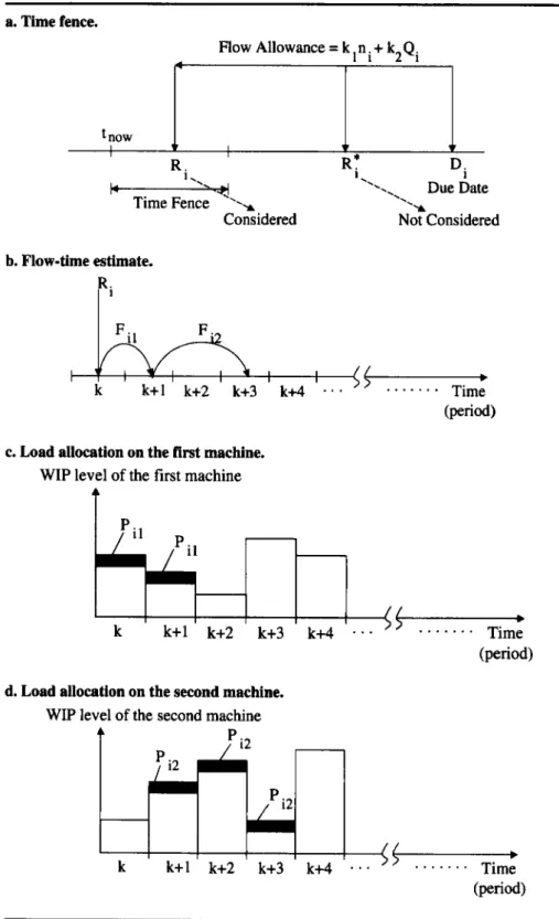
DLR is a periodic method (i.e., job release decisions are made at the begin- ning of discrete time periods). Jobs arriving during a time period are ranked accord- ing to FCFS and placed in the release pool. At the beginning of each time period (or decision point), two types of job sets are considered: (1) high-priority (or critical) jobs, whose release decisions should be made in the current period; and (2) low- priority jobs, whose releases can be postponed. If the calculated release time of a job is less than current time plus a time fence (Figure la), it is placed in the first group for further consideration. Otherwise, the job is returned to the pool and is re- evaluated at the beginning of the next period. The time fence determines a subset of the jobs that are urgent with respect to their estimated release times. Only this sub- set of the jobs are considered at the current decision point. These are the jobs that may be late if their decisions are postponed to the next time periods. The period length is the time between two consecutive decision points. In this study, eight hours of regular shift duration is used as the period length. The results of pilot runs indicate that a time period of 16 hours is quite sufficient for the time fence.
In the algorithm, the estimated (or tentative) release times are calculated for each job using equation (1) (note that the same equation was also used by Ragatz and Mabert, 1988, for the modified infinite loading mechanism, PINF).
where
Ri
D i
niQi
k,, k, = Planning factors.= Release time of job i,
= Due date of job i,
= Number of operations in job i’s routing,
= Number of other jobs waiting along job i’s routing,
Here,
Qi
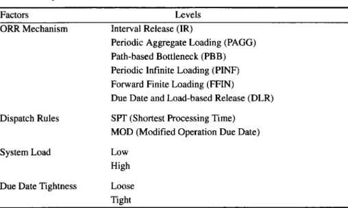
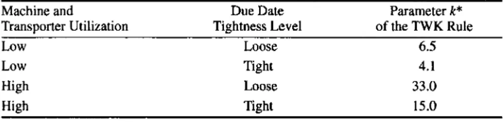
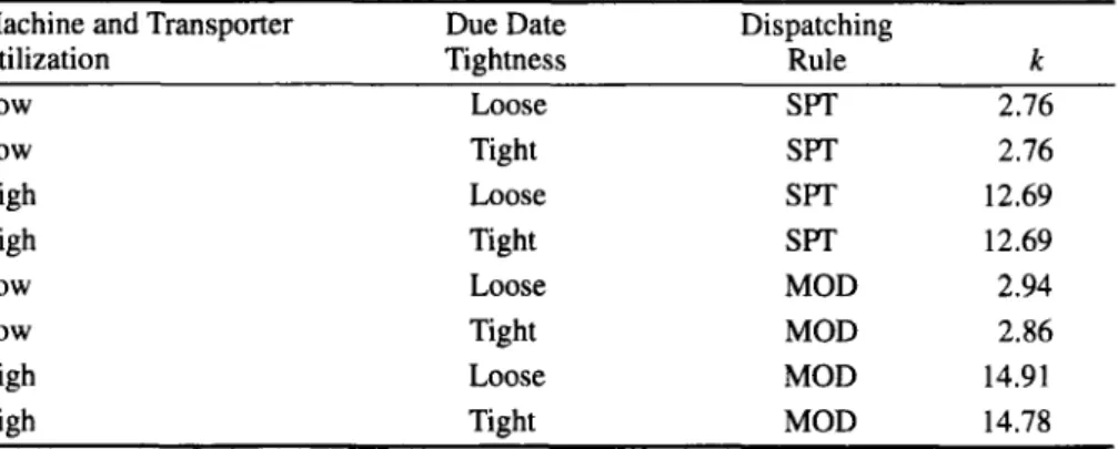
includes all jobs waiting in input queues of the machines on job i’s rout- ing, all jobs in output queues of other machines waiting to be transported, and all jobs being transported to the machines on job i’s routing. Next, we calculate theflow time (Figure 1 b) of these urgent jobs using the following equation:
FO
= k ,+
k,*
Q,, (2)where
FO Q ,
k,, k, = Planning factors.
= Flow time of thejth operation of job i,
= Number of jobs at the station where the jth operation of job i will be performed,
420 Order Review/Release in Job Shops Figure 1: Schematic view of time fence and load (or WIP) profile updates in the algorithm.
a. Time fence.
Flow Allowance= k.n.+k,O.
Y i n
b i
.,
.
i.'.
..
Due DateTime Fence '--\
.-.
mConsidered Not Considered
b. Flow-time estimate.
c. Load allocation on the first machine. WIP level of the first machine
t
k k+l k+2 k+3 k+4I
...
b Time (Period) b. . .
+(
Time (period)I
. . .
b Time (period)The sum of the flow times of all operations is equal to the total flow time of that job. These flow-time estimates include processing and transportation times as well as waiting times in input and output queues. Because a job is expected to be ready at a workstation during particular time periods, we add its processing time to this workstation’s load profile for these time periods (i.e., load is measured in time units, not in units). Note that our load profile is a time-phased load profile that shows both the current and future work loads in terms of processing times. As seen in Figures l c and Id, periods whose load (or WIP) levels increase are the ones in which the flow-time estimates of the job lie in that interval. For example, in Figure l b the flow-time estimate of the first operation of the job on the first work- station lies in k and k
+
1 and, therefore, the load level of this workstation is increased by p i l for these time periods (Figure lc). On the other hand, the load level of the second workstation is increased by pi2 for k+
1, k+
2, and k+
3, since the flow-time estimate lies in these three time periods (Figure Id).Next, we check whether the current load level in the load profile exceeds some predetermined limit at each workstation for any time period. Even if it exceeds this limit for only one period at any workstation, we stop further consider- ations with this job at this moment. This means that this job is returned to the release pool to be re-evaluated at the beginning of the next time period. We also return load level to its previous profile. However, if the limit is not exceeded, the job becomes eligible to enter the system. If the estimated release time falls before the current time, the job is released at the beginning of the time period. Otherwise, the release date of the job is frozen and the job enters the system exactly at this time. Here, the load limit represents the amount of maximum work load in hours assigned to a machine for a given time period. For the sake of simplicity, we use the same limit for each machine and determine this limit based on pilot simulation runs. The load profile is updated at each release point and each time a job completes its oper- ations. The steps of the proposed
ORR
method can be summarized as follows:1. Calculate the release time of each job in the pool.
2. If the release time of the job is less than current time plus the time fence (see Figure l), go to Step 3. Otherwise, return the job to the pool and go to Step 1 to consider the next job in the pool. If all jobs in the pool have been evaluated, then stop.
3. Calculate the operation flow time of the job.
4. Modify the load profiles of the workstations by adding the processing times of the operations to the corresponding periods’ load levels.
5 . If the load limit is not exceeded in any of the periods of the load profiles maintained for each workstation, go to Step 6. Otherwise, return the job to the pool and return to Step 1 for the next job. If all the jobs in the pool have been evaluated, stop.
6. If the release time of the job is less than the current time, release the job immediately. Otherwise, freeze the release time of the job (i.e., release the job exactly at this time).
7. Go to Step 1 to consider the next job in the pool. If all the jobs in the pool have been evaluated, stop.
422 Order Reviewmelease in Job Shops According to the steps of the algorithm, the job is not released to the system if it is expected to be too early. On the other hand, it is immediately released when expected to be tardy. In other cases, its scheduled release time is set by using the expected flow time in the system. Hence, the algorithm aims at finishing the jobs on time.
Our pilot simulation runs suggested a slightly modified version of the algo- rithm to improve on the mean flow-time measure. In this case, all jobs (not only the high-priority jobs but also the low-priority jobs) are considered in the release decisions for each time period. In other words, the time fence does not play any role, and jobs are released to the shop immediately as long as the load limits of the workstations along the process route of the jobs are not exceeded in any future time period.
EXPERIMENTAL CONDITIONS
The performance of the proposed method is studied under various experimental conditions and compared with existing ORR methods using different performance measures. Four factors are considered in the experiments: (1) ORR methods, (2) dispatching rules, (3) system utilization levels, and (4) due date tightness.
As seen in Table 1, five ORR methods and two dispatching rules are com- pared under four possible combinations of due date tightness and system load level factors. Among the
ORR
methods, DLR is the proposed method, and other meth- ods are selected because they are the more frequently used rules with different characteristics in the literature. IR is a periodic version of immediate release (IMR), where all jobs arriving during the time period are released to the system at the beginning of the next period. This rule does not use any information about shop status or characteristics of the jobs. PAGG is a load-limited ORR strategy that releases the jobs periodically, based on an aggregate measure (i.e., amount of work in hours). PBB is a relatively new load-limited release mechanism that utilizes workcenter-based information. In PBB, the job is released if the job’s processing time plus the current work load on the machine along the job’s path is below a limit determined by pilot experiments. PINF andFFIN
are two popular ORR methods that are based on calculated release times. In PINF, jobs whose release times are within the next time interval are released to the system without considering the capacity of the system. However, this capacity information is explicitly used in FFIN. The details of these parameters and their estimation methods are given in Table 2.The system load level is adjusted by changing the arrival rates. At the high level, the machine and transporter utilization rates are approximately 9 1 % and 93%, respectively. This is achieved by setting the mean time between arrival to 0.705 hours. At the low level, it is set to 0.9 hours, which results in a 66% and 63% utilization level of machines and transporters, respectively. Two levels of due date tightness are considered. The tightness level is controlled by the parameter k of the
T W K
rule (Total Work Content rule). Due dates are assigned such that the percent of tardy jobs are 10% and 30% for the loose and tight cases, respectively. These values are set in pilot runs by using FCFS (Table 3).Table 1: Experimental factors and their levels.
Factors Levels
ORR Mechanism Interval Release (IR)
Periodic Aggregate Loading (PAGG) Path-based Bottleneck (PBB) Periodic Infinite Loading (PINF)
Forward Finite Loading (FFIN)
Due Date and Load-based Release (DLR) SPT (Shortest Processing Time)
MOD (Modified Operation Due Date) Dispatch Rules
System Load Low
High Due Date Tightness Loose
Tight
The parameters (k, and k2) in equation (1) and equation (2) for the DLR method are determined for each experimental setting using regression analysis. To acquire these estimates, we collected data sets based on 1,200 observations. In order to achieve independence, observations are collected after every 50 job com- pletions. Hence, each simulation run length consists of 6,000 job completions. Each observation includes actual flow time, job characteristics, and the shop status information observed when the job arrived at the shop. Then, we fit the linear regression models (Neter, Wasserman, & Kutner, 1985) to the data. The same parameters are also used for PINF since it employs equation (2) to estimate flow times. For WIN, the parameter k is determined by regression analysis using the flow-time estimates. The values of these parameters in this study are given in Tables 4 and 5 .
Except for IR, all of the ORR methods considered in this study have one or more parameters to be specified. IR also has a parameter (period length), but it was set to eight hours as a result of pilot runs. We then used the same review period for all the methods. Note that there are seven performance metrics and eight experi- mental conditions (or factor settings), which result from the combinations of two dispatching rules, two system load levels, and two due date tightness levels. In this study, we tried to set the parameters of the ORR methods to maximize their per- formance at each condition for each measure. For example, in PAGG, we ran the simulation model for various values of the “number of jobs allowed” parameter and selected the best performer for each of 56 (8*7) different environments. The similar analysis is also carried out for the “load threshold” parameter of PBB. In
WIN and PINF, there is only a need to determine the flow-time estimation equa- tions. As explained above, these are obtained by using the regression analysis. Note that the flow time is a function of the input factors (independent of performance metrics) and, hence, the results are reported for eight factor settings (Tables 4 and 5). DLR also uses the same equations as PINF (Table 4), but it has two additional
424 Order Reviewmelease in Job Shops Table 2: ORR methods and their parameters, and sources of references.
Methods Parameters References
IR Period-length = 8 hours Panwalkar, Smith, and Dudek (1976) PAGG Period-length = 8 hours and load
allowed = found empirically
Ragatz and Mabert (1988)
PBB Load level = found empirically Philipoom, Malhotra, and Jensen ( 1993) PINF Period-length = 8 hours and Ragatz and Mabert (1988)
Ri = D i - k , * n i - k 2 * Q i FFIN Period length = 8 hours and
k value of Flow time = k
*
Processing timeBobrowski and Park (1989)
Table 3: Tightness parameter of
T W K
for experimental conditions.Machine and Due Date Parameter k*
Transporter Utilization Tightness Level of the TWK Rule
Low Loose 6.5
Low Tight 4.1
High Loose 33.0
High Tight 15.0
Di = A7;.
+
k*
TWKi, where Di = due date of job i ; AT, = arrival time of job i ; TWKi = total operation time of job i ; k = tightness parameter.parameters: time fence and load limit. As will be explained later, we test two dif- ferent values of time fence and various values of load limit to find the best param- eter settings.
The job shop simulation model is developed using the SIMAN language (Pegden, Shannon, & Sadowski, 1990). The model is run in a UNIX environment. Some of the characteristics of the shop are identical to the ones used by Melnyk and Ragatz (1988). A material handling system and finite buffer capacities are added to the classical job shop model to incorporate congestion on the shop floor. In general, congestion on the shop floor can be seen in the form of long waiting times or queues at machining centers. This undesirable situation in practice can often lead to a number of problems, such as confusion on the shop floor, difficulty in expediting and scheduling, possibility of damage due to extra handling, increased handling, wasting valuable resource times due to changes in part speci- fications, etc. The net effect of all factors is increased lead times. Hence, these fac- tors should be considered in detail by the models to realize the benefits of ORR in research settings. Also, in manufacturing systems, buffer space is often limited, and a part of lead time is due to waiting for material handling. In this study, con- gestion is modeled by considering these two important elements (i.e., finite buffer capacities and material handling system).
Table 4: Values of the planning factors used in the proposed DLR method and PINE
Machine and Due Date Dispatching
Low Loose SPT 1.91 0.55
Low Tight SFT 1.91 0.55
High Loose SFT 0.452 1.205
High Tight SPT 0.452 1.205
Low Loose MOD 1.92 0.60
Low Tight MOD 2.18 0.45
High Loose MOD 2.28 I .08
Transporter Utilization Tightness Rule kl k2
High Tight MOD 0.53 1.22
Table 5: Values of the planning factors used in forward finite loading (FFIN). Machine and Transporter Due Date Dispatching
Utilization Tightness Rule k
Low Loose SPT 2.76
Low Tight SPT 2.76
High Loose SPT 12.69
High Tight SPT 12.69
Low Loose MOD 2.94
Low Tight MOD 2.86
High Loose MOD 14.91
High Tight MOD 14.78
There are six departments in the system. Material flow is bi-directional, and job transfers are handled by five free-path transporters (i.e., forklifts). In the model, all the machines have finite input and output buffer capacities. These phys- ical maximum storage spaces are set to four units at each workcenter. There is also a separate buffer area in each department with a relatively large capacity, repre- senting a common storage area. Each job routing is purely random, with the num- ber of operations uniformly distributed between one and six.
Because the structure of the system is different from others in the literature due to the additional features (material handling and finite buffer capacities), we include some operational rules as described below. An idle transporter is dis- patched by using the modified first come, first served (MOD FCFS) rule. Accord- ing to this rule (Srinivasan & Bozer, 1992), each transporter checks all stations and picks up the oldest load in that transporter queue. If there is no move request in the system, the transporter stays idle at the station where it delivered its load. A trans-
porter request is also made whenever a job is released to the shop from the pool or whenever a job is put in the output queue. When a transporter arrives at its desti- nation station, it unloads the job if there is an empty place in the input queue. 0th- erwise, it takes it to the common storage area. If the operation is finished and there
426 Order Reviewmelease in Job Shops is no place in the output queue, the job waits on the machine until a job in the out- put queue is removed. If the number of jobs in the input queue decreases to one, and there are jobs waiting in the departmental buffer area, a transporter request is made by the station to fill the input queue of the machine.
The batch means method (Law & Kelton, 1991) is used for simulation out- put data analysis. Based on pilot experiments, the warmup period and batch size are set to 2,500 and 1,000 job completions, respectively. Each simulation run con- sists of 20 batches that result in a total of 22,500 job completions. Simulation runs are repeated for each factor combination. The Common Random Numbers (CRN) approach is also used as the variance-reduction technique to provide the same experimental condition across the runs for each factor combination. For that rea- son, a randomized block design is adopted as the tool for statistical analysis (Montgomery, 1991). The following performance measures are used to collect the relevant statistics:
Flow time = time in pool
+
time in shop, Tardiness = max (0, Cj - Di),Lateness = C j - Di,
Absolute deviation = ICj -
DJ,
where Cj and D j are completion time and due date of job i, respectively. The mean of each measure is calculated as the average of the observations collected by the simulation model. Percent tardy is also used to measure the percent of jobs finished after their due dates among all finished jobs. In addition, standard devi- ation of flow time and standard deviation of number of jobs in the shop are col- lected.
ANALYSIS
OF
RESULTSIn this section, we first compare DLR and the other ORR methods under the exper- imental conditions described earlier. Then, we test the sensitivity of these results to changes in the system parameters. Specifically, we analyze situations in which there are allowable variations in the system load and processing times.
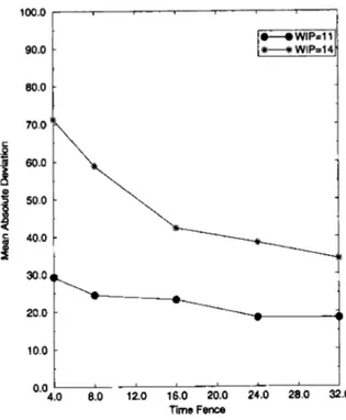
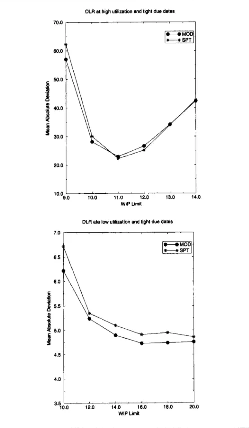
As discussed earlier, a large number of simulation runs were conducted to determine the best parameter values of the ORR methods. For DLR, we first searched for the appropriate values of the two parameters-load limit and time fence-at each experimental condition for each performance measure. The analy- sis of the simulation results reveal that the system performance is more sensitive to the load limit than to the time fence parameter. In general, a period of 16 time units appeared to be quite sufficient for the time fence parameter (Figure 2). This was chosen because the performance does not significantly improve beyond this point, whereas the computational time increases considerably as a result of more jobs involved in the release decisions. In terms of the load limit, two different values, 11 and 20, were identified for high and low utilization levels, respectively. As seen in Figure 3, the performance curves are U-shaped, indicating that there is a trade-off between the values of the load limit, especially at the high utilization rates. What
90.0 -
Figure 2: MAD performances for DLR at varying time fence values.
DLR at high utilization, tight due dates with the MOD rule
100.0, w WIP=ll W W I P = 1 4
i
l
20.0t
O"4!0 8:O 12.0 16.0 20.0 24.0 28.0 d . 0 Time FenceDLR at low utilization, loose due dates with the MOD rule
2.0 3'0
I
I 1.0 0.0'
4.0 8.0 12.0 18.0 20.0 24.0 28.0 32.0 Time Fence428 Order Review/Release in Job Shops
Figure 3: MAD performances for DLR at varying load limits.
DLR at high utilization and loose due dales 70.0
10.0
9.0 10.0 11.0 12.0 13.0 14.0 WIP Limil
DLR at low utllizatlon and loose due dates
7.0 6.5 6.0
5
fg
5.51
5.0 4.5 3 . 5 ' . ' ' ' ' ' ' ' WIP Limit4.0
Figure 3: (continued) MAD performances for
DLR
at varying load limits.-
DLR at high utilization and tight due dates
70.01 . I . I . 7 . 8 - I
20.0 10.0 9.0
L#----l
10.0 11.0 12.0 13.0 14.0WIP Limit
DLR ate low utilization and tight due dates
7.0
1
4.51
3 . 5 ’ “ ” ” ” ” 10.0 12.0 14.0 16.0 16.0 20.0 WIP Limit430 Order Review/Release in Job Shops happens is that at the lower values of the load limit, fewer jobs are released to the system, and the shop becomes underloaded. In other words, jobs spend more time in the release pool than on the shop floor. Conversely, at higher parameter values more jobs are released to the system, and the shop becomes overloaded. Hence, the performance of the system deteriorates due to congestion. Similar observations were also made for the other ORR methods.
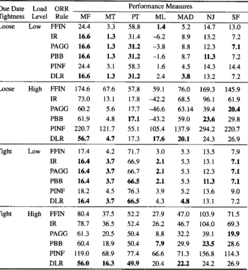
After determining the best parameters of each ORR method, we compared the methods under eight factor settings. Tables 6 and 7 show the overall perfor- mance of the methods for each performance metric. The proposed method is the best with respect to the MAD measure for which it is designed. Specifically, it yields the minimum MAD values for 144 out of 160 simulation runs. We cannot claim stochastic dominance of the proposed method, but it certainly outperforms other release methods. DLR also performs very well on the other measures. In gen- eral, it yields better mean flow time and mean tardiness performance than the other rules in the high system load case for any combination of dispatching rules and due date tightness levels. Except for three cases, it also minimizes proportion of tardi- ness. In terms of the number of jobs-in-shop measure, PBB performs slightly bet- ter than the others. It seems that PBB is quite effective in reducing the time in shop, but the flow time (which includes both time in shop and time in release pool) goes up as a result of increased waiting in the release pool. We observe that PAGG shows the best performance with respect to the standard deviation of flow time (i.e., it minimizes variations in flow time). In the case of mean lateness, there is no clear winner because the relative performances of the ORR methods change at each experimental condition.
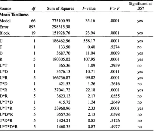
ANOVA was utilized to test the significance of factors and their interactions with respect to three measures: Mean Absolute Deviation, Mean Flow Time, and Mean Tardiness (Table 8). The Bonferroni method was also used to rank the ORR methods for some selected performance measures (Table 9). These measures were selected because they are frequently used in the literature. Because simula- tion runs were conducted for each method under the same experimental condi- tions, we included the blocking factor to represent these conditions in the ANOVA model. In Table 8, the source is significant if it has a probability value smaller than .05 in the P >
F
column. The details of the test results follow. Except for the tightness factor in the tardiness case, all factors are significant at alpha =.05. The reason for not finding the tightness factor significant is further investi- gated.
Our analysis showed that methods such as PINF and FFIN finish the jobs around their due dates. For that reason, most of the jobs become tardy regardless of their due dates’ tightness levels. At this point, we suspected that the tightness factor would become significant if these two ORR methods were excluded from the anal- ysis. Hence, we repeated the ANOVA tests without PINF and FFIN. The results of these tests confirmed our expectation. The analysis of the simulation results also showed that most of the higher order interactions are significant. This indicates that the performance of the release methods is affected by due date tightness, system load level, and dispatching rules. In general, the relative performance of the ORR methods seems to be more distinguishable at the high system load and tight due date
Table 6: Simulation results for the SPT dispatching rule.
DueDate Load ORR
Tightness Level Rule MF MT IT ML MAD NJ SF
Loose Low FFIN 24.4 3.3 58.8 1.4 5.2 14.7 13.0
IR 16.6 1.3 31.4 -6.2 8.9 13.2 7.2 Performance Measures PAGG 16.6 1.3 31.2 -3.8 8.8 12.3 7.1 PBB 16.6 1.3 31.2 -1.6 8.7 11.3 7.2 PINF 24.4 3.1 58.3 1.6 4.5 14.3 14.4 DLR 16.6 1.3 31.2 2.4 3.8 13.2 7.2
Loose High FFIN 174.6 67.6 57.8 59.1 76.0 169.3 145.9
IR 73.0 13.1 17.8 -42.2 68.5 96.1 61.9
PAGG 60.2 5.6 17.7 4 6 . 6 63.14 39.4 20.4
PBB 61.9 4.8 17.1 4 3 . 2 59.0 23.6 29.8
PINF 220.7 121.7 55.1 105.4 137.9 294.2 220.7
DLR 56.7 4.7 17.3 17.6 20.1 24.3 26.9
Tight Low FFIN 17.4 4.2 71.7 3.0 5.3 13.5 7.9
IR 16.4 3.7 66.9 2.1 5.3 13.1 7.1
PAGG 16.4 3.7 66.7 2.1 5.3 12.3 7.1
PBB 16.4 3.7 66.5 2.1 5.3 11.3 7.1
PINF 18.2 4.5 76.3 3.9 5.2 13.6 9.0
DLR 16.4 3.7 66.5 4.3 4.8 13.1 7.2
Tight High FFIN 80.4 37.5 52.2 27.9 47.0 103.9 71.5
IR 78.7 36.5 52.4 26.2 46.7 104.0 69.3
PAGG 61.3 20.5 50.4 8.8 32.2 39.1 19.9
PBB 60.4 18.9 50.4 7.9 29.9 23.5 28.6
PINF 119.0 68.9 77.4 66.6 71.3 156.8 114.3
DLR 56.0 16.3 49.9 20.4 22.2 24.2 26.9
MF: Mean Flow time; MT: Mean Tardiness; PT: Percent Tardy; ML: Mean Lateness; MAD: Mean Absolute Deviation; NJ: Average Number of Jobs in the Shop; SF: Standard Deviation of Flow time.
*Boldface numbers represent the cases in which the results are significant at alpha = .05.
the MAD and tardiness measures. In this case, we note that the performance of
ORR
methods can be improved by using the due-date-based rule MOD.
We also applied the Bonferroni test (at alpha = .05) to rank the
ORR
meth- ods. This test compares all pairs of means (i.e., mean performance ofORR
methods) and arranges them in descending order. Because significant interac- tions were identified between the factors, the comparisons are performed for each factor.
In Table 9, the methods that are statistically different from each other are labeled with different letters. For example, at low load level with loose due dates,
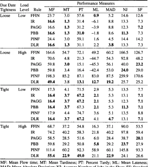
432 Order Review/Release in Job Shops Table 7: Simulation results for the MOD dispatching rule.
DueDate Load
Tightness Level Rule MF MT IT ML MAD NJ SF
Loose Low WIN 23.7 3.0 57.6 0.9 5.2 14.6 12.6
IR 16.6 1.3 31.4 -6.1 8.8 13.3 7.3 Performance Measures PAGG 16.6 1.3 31.2 -3.9 8.8 12.3 7.2 PBB 16.6 1.3 31.0 -1.8 8.6 11.3 7.3 PINF 24.4 3.0 59.1 1.6 4.5 14.4 14.2 DLR 16.6 1.3 31.1 2.2 3.8 13.3 7.3
Loose High FFIN 164.6 54.7 72.1 49.2 60.2 166.5 126.7
IR 70.6 4.8 21.3 -44.7 54.3 92.8 48.2
PAGG 59.8 3.0 15.1 -45.3 56.1 40.0 23.2
PBB 59.8 3.4 16.4 -42.4 53.0 24.0 29.0
PINF 198.3 85.2 87.1 83.0 87.5 259.9 170.6
DLR 49.4 3.8 13.1 12.7 19.2 25.7 25.2
Tight Low FFIN 17.3 4.1 71.5 2.9 5.3 13.5 7.7
IR 16.4 3.7 67.2 2.1 5.3 13.1 7.1
PAGG 16.4 3.7 67.2 2.1 5.3 12.3 7.1
PBB 16.4 3.7 67.3 2.1 5.3 11.3 7.1
PINF 17.9 4.4 74.7 3.6 5.1 13.5 8.8
DLR 16.4 3.7 67.2 4.1 4.7 13.1 7.1
Tight High FFIN 68.7 37.2 54.8 16.3 37.1 90.0 53.5
IR 74.2 40.2 58.3 21.8 40.2 97.8 59.4
PAGG 58.5 28.5 51.6 6.0 28.4 38.7 20.1
PBB 59.8 29.2 50.8 5.8 29.2 23.7 27.9
PINF 111.4 60.2 92.3 58.9 60.1 145.8 93.3
DLR 55.4 22.9 49.0 21.1 22.9 24.1 26.6 MF: Mean Flow time; MT: Mean Tardiness; PT: Percent Tardy; ML: Mean Lateness; MAD: Mean Absolute Deviation; NJ: Average Number of Jobs in the Shop; SF: Standard Deviation of Flow time.
*Boldface numbers represent the cases in which the results are significant at alpha = .05.
whereas DLR, labeled with D, performs significantly better than others. The test results indicate that the relative ordering of the ORR methods changes slightly from one condition to another. In general, DLR is the best method, followed by PBB and PAGG. The rules IR, PINF, and FFIN perform poorly. Specifically, DLR with the MOD dispatching rule is the best method for the mean absolute deviation. With the SIT rule, DLR is the best method for only the loose due dates. When the due dates are tight, it yields smaller MAD values even though the difference between them is not significant.
In terms of the mean flow time and tardiness measures, the Bonferroni test does not identify significant differences among DLR, PBB, and PAGG, but DLR
Table 8: ANOVA results for three performance measures.
Significant at Source df Sum of Squares F-value P > F .05? Mean Absolute Deviation
Model 66 880379.48 34.28
.om
1 YesError 893 347502.67
Block 19 63203.27 8.55
.om
1 YesU 1 487858.92 1253.68 .om1 Yes
T 1 39009.5 1 100.25
.om
1 YesD 1 6802.20 17.48 .oO01 Yes
R 5 98576.77 50.66 .om1 Yes
U*T 1 30756.32 79.04 .oO01 Yes
U*D 1 6611.37 16.99
.om
1 YesU*R 5 9999 1.54 51.39 .oO01 Yes
T*D 1 1712.99 4.40 .0362 Yes
T*R 5 13961.08 7.18
.om
1 YesD*R 5 5935.39 3.05 .0097 Yes
U*T*D 1 1690.46 4.34 .0374 Yes
U*T*R 5 13267.20 6.82 .o001 Yes
U*D*R 5 5979.70 3.07 .0093 Yes
T*D*R 5 2494.48 1.28 .2694 no
U*T*D*R 5 2528.2 1 1.30 .2619 no
Mean Flow Time
Error 893 394762.16
Model 66 2649620.29 90.81 .oO01 Yes
Block 19 306292.78 36.47
.om
1 yesU 1 1207247.76 2730.94 .oO01 Yes
T 1 64255.37 145.35 .oO01 Yes
D 1 2 185.90 4.94 .0264 Yes
R 5 422042.4 1 190.94 .OOO1 Yes
U*T 1 48008.55 108.60 .oO01 Yes
U*D 1 2123.34 4.80 .0287 Yes
U*R 5 344164.98 155.71 .oO01 Yes
T*D 1 118.87 0.27 .6042 no
T*R 5 140608.74 63.61 .om1 Yes
D*R 5 1637.73 0.74 S929 no
U*T*D 1 122.18 0.28 S992 no
U*T*R 5 108 1 53.90 48.93
.om
1 YesU*D*R 5 1506.16 0.68 .6376 no
T*D*R 5 560.89 0.25 .9380 no
434 Order Reviewmelease in Job Shops
Table 8: (continued) ANOVA results for three performance measures.
~~
Significant at Source df Sum of Squares F-value P > F .05?
Mean Tardiness
Model 66 775 100.95 35.16
.om1
YesError 893 298315.58
Block 19 15 1928.76 23.94
.ooo
I YesU 1 186462.56 558.17 .OoOl Yes
T 1 133.50 0.40 S274 no
D 1 3687.70 11.04 ,0009 Yes
R 5 180305.02 107.95 .000 1 Yes
U*D 1 3576.13 10.71 .m11 Yes
U*R 5 166736.87 99.82
.ooo
1 YesT*D 1 421.53 1.26 ,2616 no T*R 5 37041.72 22.18
.ooo
1 Yes D*R 5 3623.13 2.17 .0555 no U*T*D 1 415.72 1.24 .2649 no U*D*R 5 3557.36 2.13 .0598 no T*D*R 5 1424.2 1 0.85 .5 126 no U*T*D*R 5 1460.35 0.87 A977 no U*T 1 365.36 1.09 .2959 noU*T*R 5 33960.96 2.33 .om1 Yes
U: Utilization; T: Due date tightness; D: Dispatching rule; R: Release mechanism
still yields more than 10% improvement over the second best method. This may be partly due to the comparison of all six ORR methods at once (i.e., multiple statements)
.
We further compare DLR with PBB to see if the proposed method provides any advantage over the most competitive rule, PBB, for the mean tardiness and flow-time metrics. Specifically, we compare the mean performance of DLR and PBB by using the paired t-test (see Table 10; the results that are significant are labeled by "*"). The results indicate that there is no statistical difference between these two methods when the system load is low. This is understandable because at this load level, the methods may not have enough opportunity to show different performances since there are only a few jobs on the shop floor. Thus, these results are not shown in Table 10. But when we have the high system load and due date is loose,
DLR
with theMOD
dispatching rule performs better than PBB for both the mean tardiness and mean flow-time metrics. The proposed method is also better than PBB for the mean flow-time measure with the SPT rule.Table 9: Bonferroni’s multiple range test results.
~~ ~ ~ ~ _ _ _ _ _
SIT MOD
Load
DueDate Level Ranking Mean ORR Ranking Mean ORR
Mean Absolute Deviation
Loose Low A 8.88 IR A 8.81 IR A 8.76 PAGG A 8.78 PAGG A 8.62 PBB A 8.57 PBB B 5.22 FFIN B 5.20 FFIN C 4.49 PINF C 4.50 PINF D 3.79 DLR D 3.77 DLR
Loose High A 137.99 PINF A 87.56 PINF
B 76.04 €FIN AB 60.27 FFIN
B 68.49 IR B 56.19 PAGG
B 63.14 PAGG B 54.35 IR
B 59.08 PBB B 53.05 PBB
C 20.13 DLR C 19.23 DLR
Tight Low A 5.38 IR A 5.34 FFIN
A 5.35 PAGG AB 5.31 PBB
B 5.35 PBB AB 5.31 PAGG
B 5.32 FFIN AB 5.30 IR
B 5.25 PINF B 5.15 PINF
B 4.85 DLR C 4.73 DLR
Tight High A 71.31 PINF A 60.18 PINF
B 47.08 WIN B 40.23 IR
B 46.75 IR B 37.17 FFIN
C 32.28 PAGG BC 29.20 PBB
C 29.98 PBB BC 28.47 PAGG
C 22.25 DLR C 22.94 DLR
Mean Flow Time
Loose Low A 24.39 PINF A 24.36 PINF
B 23.95 FFIN B 23.72 FFIN
C 16.57 IR C 16.63 PAGG
C 16.55 PAGG C 16.60 DLR
C 16.55 PBB C 16.59 IR
C 16.55 DLR C 16.57 PBB
Loose High A 220.76 PINF A 198.35 PINF
B 174.60 FFIN B 164.61 FFIN
C 73.08 IR C 70.65 IR
C 61.90 PBB D 59.87 PAGG
C 60.20 PAGG D 59.84 PBB
436 Order Reviewmelease in Job Shops Table 9: (continued) Bonferroni's multiple range test results.
SIT MOD
Load
DueDate Level Ranking Mean ORR Ranking Mean ORR Mean Flow Time (continued)
Tight Low A 18.24 FFTN A 17.99 PINF
B 17.42 PINF B 17.31 FFIN
C 16.45 IR C 16.46 PAGG
C 16.44 DLR C 16.45 DLR
C 16.43 PBB C 16.44 IR
C 16.43 PAGG C 16.43 PBB
Tight High A 118.98 PINF A 111.37 PINF
B 80.40 FFIN B 74.25 IR B 78.70 IR B 68.80 FFIN C 61.27 PAGG C 59.84 PBB C 60.36 PBB C 58.52 PAGG C 56.02 DLR C 55.45 DLR Mean 'hrdiness
Loose Low A 3.21 FFIN A 3.09 FFIN
A 3.08 PINF A 3.06 PINF
B 1.36 PAGG B 1.34 PAGG
B 1.36 IR B 1.34 IR
B 1.35 PBB B 1.32 PBB
B 1.34 DLR B 1.32 DLR
Loose High A 121.70 PINF A 85.28 PINF
B 67.60 FFIN B 54.74 FFIN
C 13.10 IR C 4.8 1 IR
C 5.60 PAGG C 3.78 DLR
C 4.83 PBB C 3.38 PBB
C 4.78 DLR C 3.06 PAGG
Tight Low A 4.56 PINF A 4.40 PINF
B 4.23 FFIN B 4.16 FFIN
C 3.73 IR C 3.73 PAGG
C 3.73 PAGG C 3.7 1 IR
C 3.73 DLR C 3.71 PBB
C 3.71 PBB C 3.71 DLR
Tight High A 68.95 PINF A 60.18 PINF
B 37.50 FFIN B 40.23 IR
B 36.50 IR B 37.16 FFIN
C 20.55 PAGG BC 29.20 PBB
C 18.95 PBB BC 28.47 PAGG
Table 10: Paired t-test results for DLR and PBB.
Dispatching Due Date
Rule Utilization Tightness Mean SE Mean T P-value
Mean Flow Time
SPT high loose 5.55 2.08 2.4 1 .02*
SPT high tight 10.40 2.08 4.99 .001*
MOD high loose 4.33 1.77 2.45 .02*
MOD high tight 4.34 2.55 1.69 .10
Mean Tardiness
SPT high tight -0.39 0.65 -0.60 .56
MOD high loose 2.58 1.14 2.26 .03*
MOD high tight 2.63 1.14 2.30 .03*
Boldface numbers significant at alpha = .05.
*Significant results.
SPT high loose 0.72 1.32 0.552 .58
SENSITIVITY OF THE RESULTS TO LOAD AND PROCESSING-TIME VARIATIONS
In practice, the demand for products is not constant, but changes over time depend- ing on market conditions. In some cases, the demand rate displays a seasonal vari- ation and, hence, the interarrival time between customer orders changes from period to period. We call this situation load variation (LV) and model it by manip- ulating the parameter of the interarrival time distribution. We change the mean time between arrivals at every 250Job arrival. The amount of change (or variation) is drawn from a uniform distribution with a range of [-1, 11, and then scaled by a load variation parameter (or a variation percentage). Based on our pilot experi- ments, we set these medium and high levels of variation to 10% and 20%, respec- tively. We assume that the low-level load variation corresponds to the no-variation case from the base experimental condition described earlier.
In the simulation model, we sample processing times from one of the Erlang distribution functions. This is a common procedure in the literature to model uncertainty in machining processes. However, random processing times in simu- lation models can account for only a part of total variability in the processes; it may represent variations in customer orders, material, tools, machines, and machining conditions, etc. There are other factors that add to the randomness. Actual proc- essing times realized on the shop floor can be quite different from estimated quan- tities. This could be due to variations in machines, tools, workers, and materials. In order to model this situation, we perturb the processing times. In the simulation model, the estimates are still drawn from the Erlang distribution. However, only some percentages (plus or minus) of the sampled quantities are used as actual proc- essing times. This adjustment is made similar to the load variation case. In the experiments, we used the 20% and 40% levels to represent the medium- and high- level processing time (PV) variation cases (e.g., in the 20% case, actual processing
438 Order Reviewflelease in Job Shops time of a particular operation can be +20% different from estimated quantities).
Again, the no-variation case corresponds to the low level of this factor.
The simulation results indicate that both the load variation and processing- time variation have a significant impact on system performance. As seen in Figure 4, which depicts the overall results by considering every experimental con- dition, each performance measure degrades considerably as the variation levels increase. This degradation was more apparent for the high utilization rate level. We also observed that the load variation has more impact on the system performance than the processing-time variation.
These observations are also verified by the statistical tests (i.e., ANOVA and Bonferroni tests). The test results show that differences between the ORR methods become more significant as the amount of variation increases. In many cases, we observe an increasing spread in performance among the ORR methods (see Fig- ures 5 and 6 for the overall results-average performance of the rules using the entire data set). Specifically, the performances of rules such as PINF, FFIN, IR, and PAGG deteriorate more than DLR and PBB. We also note that the relative ranking of the ORR mechanisms remains the same in the variation case.
DISCUSSION AND CONCLUDING
REMARKS
In this paper we have developed a new order release method for shop floor control systems. The results of simulation experiments indicate that DLR with the MOD dispatching rule outperforms other ORR methods with respect to the MAD mea- sure. When the dispatching rule is SPT, it displays better performance at loose due dates. When the rule is SPT and due dates are tight, it still yields numerically smaller MAD values even though the difference is not significant. This shows the advantage of using both load and due date information simultaneously to improve system performance. This finding is consistent with the current practice of man- ufacturing managers who use system-related information (i.e., current system load and capacity utilization) as much as the due-date-based job priorities to achieve on-time deliveries. In terms of the mean tardiness measure, DLR per- forms better than the most competitive rule, PBB, especially when the dispatch- ing rule is MOD, due date is tight, and the system load is high. Because the parameters of each ORR method were set to maximize the performance for each condition, this study should be viewed as one that optimizes a single performance metric.
For the first time, the ORR methods were compared at varying levels of sys- tem load and processing times. As expected, the performance of the methods dete- riorates as the variation increases. Nevertheless, DLR was the most robust method. The difference between the ORR methods becomes more significant as the varia- tion increases. This means that a more effective way of releasing jobs to the system can reduce the negative effects of the variability and uncertainty in the system.
Another finding is that controlled release is a better policy than the immedi- ate release. This was particularly shown by the improved performance of DLR over IR for the MAD and mean flow-time measures when the system load was high, regardless of the due date tightness level. This means that managers should be very careful in choosing the right ORR methods when the system experiences
Figure 4: Effects of load and processing-time variation with the DLR and MOD rules. 160.0 140.0 120.0
I
100.0D
80.0 0 80.0 40.0 20.0 0.0 Overall ResultsI
Medium High ' None Load variation (LV) Overall Results 160.0"
:I
0.0 None Medium High
440
Figure 5: Performance of
ORR
methods under load variation.Order Reviewmelease in Job Shops
240.0 220.0 200.0 180.0 160.0 60.0 40.0 20.0 0.0 200.0 180.0 180.0 140.0
c
80.0 80.0 40.0 20.0 0.0None Medium High
Load variation (LV)
None Medium High
Figure 5: (continued) Performance of ORR methods under load variation. 200.0 180.0 160.0 140.0 .Il .? 120.0
4
100.0 di
c
OO.O 60.0 40.0 20.0 0.0*
*
None Medium H i h Load variation (LV) 340.0r
320.0 : 300.0 : 260.0‘r
260.0 : 240.0 : 220.0 ; 200.0 : B 180.0 1p
160.0;
=
140.0;
120.0 : 100.0 - 80.0 80.0 20.0 40.0I
-
i
1 Medium High 0.01
None Load variation (LV)442
Figure 6: Performance of ORR methods under processing-time variation.
Order Reviewfielease in Job Shops
140.0 -
Processing-time variation (PV) 20.0
20.0 I-
-
O'O
'
Nine Medium HighFigure 6: (continued) Performance of ORR methods under processing-time variation. 80.0 60.0
B
3
I 20.0 0.0 200.0 180.0 160.0 140.0il
120.0!
=
100.0 9 80.0 80.0 40.0 20.0 0.0 M FFlN W PlNFNone Medium High
Processing-time variation (PV)
W FFlN
W PlNF
None Medium High
444 Order Review/Release in Job Shops
very high workload. We also noted that differences between the ORR methods become more apparent with high utilization rates and/or tight due date conditions. This means that in today’s highly competitive environments with several con- straining resources, the ORR function is even more important than in the past.
The proposed method is based on a load-limiting strategy and utilizes due date information. It maintains a time-phased load profile for each machine and makes the release decision according to this profile by considering the job charac- teristics and the system information. It tries to achieve on-time deliveries while keeping the system load or congestion on the shop floor at a reasonable level. There are four parameters of DLR. The first two parameters are regression coeff- cients. These are determined in the same way as in FFIN and PINE The other two are the load limit and time fence parameters, and can be determined by either using the real data or simulated data. The latter approach is easier to implement. With today’s computing systems and software packages, the data collection and analysis can be done with moderate effort. The proposed method may create a computa- tional burden if the system is manually operated. But one does not have to change these parameters frequently. The analysis can be done whenever there is a need for that (i.e., when there is a considerable change in master plans, operation times, or major shifts in production practice). Besides, the other ORR methods have one or more parameters that may require similar estimations.
Even though the main emphasis of this study was on the ORR function, we also tested two dispatching rules. Our results indicate that MOD performs better than SPT with respect to due-date-related criteria. Also, the use of a due-date-ori- ented dispatching rule positively affected the performance of the ORR methods. This observation again highlights the importance of due date information for the effective use of ORR methods in practice. Another conclusion is that dispatching (or scheduling) is still as important as order reviewhelease. Hence, managers of today’s production systems should control these two functions simultaneously. Our personal experience with manufacturing companies is that managers release orders to the system regardless of the current system status because they believe that these orders will be processed anyway after release. However, this causes congestion and confusion on the shop floor and complicates the dispatching task. Unfortunately, better scheduling in such a hopeless situation cannot help to correct the problems. As a result, the system performance deteriorates quickly. In order to alleviate these problems, dispatching and ORR functions should be harmoniously operated.
As noted above, the system load and job due date information is important for the successful application of the ORR policies. This point should be considered in future research. In addition, there should be further studies to test the ORR methods under different experimental conditions so that practitioners will have more complete knowledge about the choice of right ORR methods. It would be interesting also to determine the robustness of ORR methods to changes in due dates, cancellations of orders, and machine breakdowns so that practitioners can have more confidence in using ORR methods. Several other research topics are also possible as extensions from the structure of the proposed algorithm (e.g., one can develop and test different release time formulas that utilize both the previous jobs and processing-time information). [Received: January 28, 1998. Accepted: